Entropy and Temperature of a
Quantum Carnot Engine
Abstract
It is possible to extract work from a quantum-mechanical system whose dynamics is governed by a time-dependent cyclic Hamiltonian. An energy bath is required to operate such a quantum engine in place of the heat bath used to run a conventional classical thermodynamic heat engine. The effect of the energy bath is to maintain the expectation value of the system Hamiltonian during an isoenergetic process. It is shown that the existence of such a bath leads to equilibrium quantum states that maximise the von Neumann entropy. Quantum analogues of certain thermodynamic relations are obtained that allow one to define the temperature of the energy bath.
Keywords: quantum-mechanical engine; von
Neumann entropy;
thermodynamic equations of state
1 Introduction
A classical thermodynamic heat engine converts heat energy into mechanical work by using a classical-mechanical system in which a gas expands and pushes a piston in a cylinder. Such a heat engine obtains its energy from a high-temperature heat reservoir. Some of the energy taken from this reservoir is converted to mechanical work. A heat engine is not perfectly efficient, so some of the energy taken from the heat reservoir is not converted to mechanical energy, but rather is transferred to a low-temperature reservoir (Planck 1927).
A classical heat engine running between a high-temperature reservoir and a low-temperature reservoir achieves maximum efficiency if it is reversible. While it is impossible to construct a working heat engine that is perfectly reversible, in the early 19th century Carnot proposed a mathematical model of an ideal heat engine that is not only reversible but also cyclic (Carnot 1824). The Carnot engine consists of a cylinder of ideal gas that is alternately placed in thermal contact with high-temperature and low-temperature heat reservoirs whose temperatures are and , respectively.
Instead of a classical system of gas, we consider here a quantum-mechanical system of consisting a single particle in contact with a reservoir. The system is described by a time-dependent cyclic Hamiltonian. The statistical ensemble of many such identically-prepared systems that we consider here is characterised by a density matrix. We assume that the system interacts weakly with its environment. It is known that it is possible to extract work from such a system (e.g., Geva Kosloff 1994; Kosloff, et al. 2000).
In particular, if the evolution of the density matrix is reversible, then we can construct a quantum-mechanical Carnot engine (Bender, et al. 2000). The purpose of the present paper is to investigate the properties of quantum Carnot engine. This is of importance because it improves our understanding of the relationship between thermodynamics and quantum mechanics, an area of considerable interest in quantum theory (e.g., Leff Rex 1990).
This paper is organised as follows: First, we explain the concept of a quantum engine by generalising the two-state model considered by Bender, et al. (2000) to an infinite-state square-well model and derive equations of states for isoenergetic and adiabatic processes. These results lead naturally to the quantum analogue of the Clausius equality for a reversible cycle. We show that, unlike the result in classical thermodynamics, the Clausius relation obtained here is not based on the change of entropy.
We then introduce the von Neumann entropy and obtain the maximum entropy state subject to isoenergetic requirements. We demonstrate that the maximum von Neumann entropy is consistent with the thermodynamic definition of entropy, as well as the equations of states for quantum Carnot cycle. As a consequence, we are able to determine the temperature of the energy bath directly from two of the diagonal components of the density matrix. We conclude by discussing several open problems.
2 Quantum Carnot cycle
We can construct a simple quantum engine using a single particle of mass confined to an infinite one-dimensional square-well potential whose volume (width) is . For any fixed it is easy to solve the time independent Schrödinger equation to determine the energy spectrum of the system:
| (1) |
We assume that the width of the well initially is and that the initial energy of the system is a fixed constant . The initial state of the system is a linear combination of the energy eigenstates . Thus,
| (2) |
where , and is bounded below by . Note that the pure state characterises a typical element of the ensemble, whose statistical property is thus determined by the density matrix, given, in the energy eigenstates, by .
Starting with the above initial configuration, we define a quantum cycle as follows: First, the well expands isoenergetically; that is, the width of the well increases infinitely slowly while the system is kept in contact with an energy bath. Note that the quantum adiabatic theorem (Born Fock 1928) states that if the system were isolated during such an expansion, the system would remain in its initial state. That is, the absolute values of the expansion coefficients would remain constant. Thus, if the system were isolated, the energy of the system (the expectation value of the Hamiltonian) would decrease like .
However, during this expansion, we simultaneously pump energy into the system in order to compensate this decrease of the energy. Thus, the well, which can be viewed as a one-dimensional piston, expands in such a way that the expectation value of the Hamiltonian is held constant by exciting higher energy states. This implies that, unlike the isothermal process in classical thermodynamics, the temperature of the ‘bath’ in an isoenergetic process is in fact changing. The explicit volume dependence of temperature is derived in Section 5.
During such an isoenergetic expansion, mechanical work is done by the force (one-dimensional pressure) on the walls of the well. The contribution to this force from the th energy eigenstate is
| (3) |
Hence the force is given by the expectation value . Using the relation and Eq. (2), we obtain the equation of state during an isoenergetic process:
| (4) |
This result is identical to the corresponding equation of state for an isothermal process of a classical ideal gas, if we make the identification . Note that the expansion coefficients of the wave function change as a function of the width while the well expands isoenergetically from to .
Second, the system expands adiabatically. During an adiabatic process the eigenstates change as a function of , but the values remain constant. Therefore, the expectation value of the Hamiltonian decreases during the process because each decreases with increasing while all are kept fixed. The force in this case is determined by differentiating the energy with respect to . Thus, the equation of state during an adiabatic process for the square-well potential is
| (5) |
which is a quantum analogue of the corresponding equation for a classical ideal gas. The system expands adiabatically until its volume reaches . At this point the expectation of the Hamiltonian decreases to . Because the squared coefficients of the wave function remain constant during an adiabatic process, the value of is given by .
Following the adiabatic expansion, the system is compressed isoenergetically until , with the expectation value of the Hamiltonian fixed at , and finally it is compressed adiabatically until the width of the system returns to its initial value . This cycle is reversible, and we find that the efficiency of the quantum engine is given by
| (6) |
a formula analogous to the classical thermodynamic result of Carnot (1824).
3 Quantum Clausius relations
We have demonstrated above an example of a quantum system with a slowly-changing time-dependent Hamiltonian from which work can be extracted. The key concept introduced here is an energy bath that maintains the expectation value of the Hamiltonian. This idea can be developed further to establish the quantum counterparts of the classical thermodynamic relations. To begin with, let us first consider the theorem of Clausius.
During an isoenergetic expansion, the amount of energy transferred to the system to maintain the expectation of the Hamiltonian is determined by the integral
| (7) |
where . The amount of energy absorbed during an isoenergetic compression can be determined similarly with the result . Thus, for a closed, reversible cycle we obtain the quantum Clausius equality
| (8) |
because for a closed cycle.
In classical thermodynamics the Clausius equality states that the total change of entropy in a reversible cycle is zero, where the differential of entropy is the ratio of the absorbed heat and the bath temperature. Therefore, the relation (8) suggests that in quantum mechanics the entropy change in an isoenergetic process might be given by , the ratio of the absorbed energy to the bath energy. However, as we show below, this quantity does not determine the amount of entropy change, and hence the quantum Clausius relation is not a condition for entropy. Instead, it merely implies that the total energy absorbed, for given bath energies, must vanish in a reversible cycle. If the cycle is irreversible, then we have .
4 Entropy maximisation
To understand the change of entropy in a quantum Carnot cycle we consider the von Neumann entropy
| (9) |
associated with the density matrix , expressed in terms of the energy eigenstates. Let us first consider the isoenergetic process and introduce a scaling parameter such that . Then, during an isoenergetic process the probability that the system is in the th eigenstate changes in , subject to the constraints
| (10) |
where we have chosen units in which and taken the initial condition . There are infinitely many combinations of satisfying these constraints, each of which determines the entropy. Hence, quantum mechanically it appears that any one of such states is allowed in an isoenergetic process. However, there is a unique density matrix that satisfies the thermodynamic requirement of the change of entropy, and this is the state that maximises the von Neumann entropy.
To show this, we must determine the density matrix that maximises the entropy subject to the constraints (10) and then obtain the associated entropy . We can perform this maximisation directly without using Lagrange multipliers. The two constraints in (10) imply that two of the diagonal components, say and , of the density matrix are determined. Therefore, if we differentiate the constraints (10) with respect to , we find that
| (11) |
Solving these linear equations, we obtain
| (12) |
for all . Substituting these expressions into and solving for , we get
| (13) |
which is also valid for any choice of .
Given the maximum entropy state (13), we can now reexpress the constraints in the form
| (14) |
where we have defined . This is obtained by substituting (13) in (10), solving for , and equating the resulting expressions. Similarly, using the parameter , the state represented in (13) can be expressed as
| (15) |
Therefore, the corresponding von Neumann entropy is
| (16) |
This is independent of because of the identity
| (17) |
Thus, given the width scale of the potential well, the relation (14) determines the value of , from which we can determine both and as functions of the single length scale parameter .
We can now analyse the entropy associated with the isoenergetic process. We note first that the change of entropy associated with (16) does not agree with the quantity . More specifically, we verify that only asymptotically for large values of , that is, large energies, the two quantities are proportional to each other. In particular, because the value of in (16) is independent of the choices of and , we can set and without loss of generality. Then, asymptotically we have for large . Furthermore, the maximum entropy state satisfies for all . Therefore, and for large values of we use the asymptotic relation
| (18) |
to determine the entropy change. The result gives when the width changes from to . On the other hand, from (7) we deduce that for any value of . This establishes the asymptotic proportionality. However, does not in general determine the entropy change.
5 Equilibrium-state temperature
Next, we show that the maximum von Neumann entropy (16) is consistent with thermodynamic considerations. Recall that an isoenergetic process must proceed infinitely slowly in order that the energy bath at any point during the process be in thermal equilibrium. Thus, this process requires an infinite amount of time to be realised. Then from the principles of statistical mechanics (Schrödinger 1952) we deduce that, if we set , the temperature of the bath is given by . This is because we can make the identification in Eq. (15). On the other hand, temperature is given in thermodynamics by the formula
| (19) |
where . In the present consideration we have from the equation of state and the relation , while from (16) we find that . Therefore, the thermodynamic definition of temperature in (19) gives
| (20) |
which agrees with the statistical mechanical consideration above. We conclude therefore that the maximum von Neumann entropy determines the density matrix of the system in an isoenergetic process. Furthermore, the temperature of the energy bath can be obtained from (20), where is determined by any two diagonal components , of the density matrix. In particular, the temperature of the bath changes continuously in during an isoenergetic process, even though the energy of the system is held fixed.
We now consider the adiabatic process. In this case, there is no net energy absorbed by the system, so the thermodynamic entropy remains constant. On the other hand, because the diagonal components of the density matrix are constant during an adiabatic process, the von Neumann entropy (9) also remains constant, in agreement with the thermodynamic consideration.
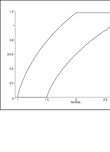
These results can be expressed by the phase diagram in the entropy-volume plane, as shown in figure 1. The diagram shows that the thermodynamic constraint is satisfied by, and only by, the maximum von Neumann entropy. Thus, we emphasise that the quantum state corresponding to the maximum von Neumann entropy, as obtained by microscopic analysis, is entirely consistent with the thermodynamic equations of states.
6 Discussion
In the analysis above we have considered only the square-well potential model, which can be interpreted as the quantum analogue of the classical ideal gas. A natural extension of this work would be to consider other Hamiltonians. For example, for a harmonic potential whose energy eigenvalues are , a dimensional argument shows that the characteristic length scale is given by . Therefore, the equations of states for the harmonic potential become identical to those for the square-well potential, although the volume dependence of the entropy is different from (16). For other Hamiltonians, however, the equations of states are not in general identical to those obtained here, and it would be interesting to find explicit examples of other models exhibiting nonideal behaviours.
Another important issue is to understand whether there is any role played by the geometric phases, a concept that does not have an analogue in the classical Carnot cycle. Although the quantum Carnot engine is indeed cyclic in terms of , the coefficients of the wave function of any one of the representatives in the ensemble inevitably pick up geometric phases as the system goes through a cycle. Therefore, strictly speaking, the wave function is not cyclic in the quantum Carnot cycle. The question then is whether there is any physically observable evidence of the geometric phase in the present context, and if so, how do we represent that in the mixed state context (cf. Uhlmann 1996).
Finally, another interesting idea that should be studied is the possibility of constructing a cyclic quantum engine (or a quantum refrigerator by reversing the cycle) that requires only a finite amount of time to complete. Note that each cycle of a classical Carnot engine is infinitely long. However, in quantum mechanics, it is known, for example, that by choosing a specific form of time dependent Hamiltonians, it is possible to construct a quantum-mechanical cycle in an essentially arbitrary short time scale (Mielnik 1986). It would be of interest to determine if such an idea can be applied to create a finite-time Carnot engine, or whether such dynamics would be incompatible with the requirement of maximising the von Neumann entropy. An analysis on the performance of finite-time cycle in the presence of friction has been studied in Feldmann Kosloff (2000).
We wish to express our gratitude to A. Howie and M. F. Parry for stimulating discussions. DCB gratefully acknowledges financial support from The Royal Society. This work was supported in part by the U.S. Department of Energy.
References
- [1]
- [2] Allahverdyan, A. E. Nieuwenhuizen, Th. M. 2000 Phys. Rev. Lett. 85, 1799.
- [3]
- [4] Bender, C. M., Brody, D. C. Meister, B. K. 2000 J. Phys. A33, 4427.
- [5]
- [6] Born, M. Fock, V. 1928 Zeits. f. Physik 51, 165.
- [7]
- [8] Carnot, S. 1824 Réflexions sur la Puissance Motrice du Feu et sur les Machines Propres a Développer Cette Puissance, Paris: Chez Bachelier.
- [9]
- [10] Feldmann, T. Kosloff, R. 2000 Phys. Rev. R 61, 4774.
- [11]
- [12] Geva, E. Kosloff, R. 1994 Phys. Rev. E 49, 3903.
- [13]
- [14] Kosloff, R., Geva, E. Gordon, J. M. 2000 J. App. Phys. 87, 8093.
- [15]
- [16] Leff, H. S. Rex, A. F. (eds.) 1990 Maxwell’s Demon, Entropy, Information, Computing, Bristol: Adam Hilger.
- [17]
- [18] Mielnik, B. 1986 J. Math. Phys. 27, 2290.
- [19]
- [20] Planck, M. 1927 Treatise on Thermodynamics, London: Longmans, Green and Co.
- [21]
- [22] Schrödinger, E. 1952 Statistical Thermodynamics, Cambridge: Cambridge University Press.
- [23]
- [24] Uhlmann, A. 1996 J. Geom. Phys. 18, 76.
- [25]