Quantum Networks for Concentrating Entanglement

Abstract

If two parties, Alice and Bob, share some number, $n$, of partially entangled pairs of qubits, then it is possible for them to concentrate these pairs into some smaller number of maximally entangled states. We present a simplified version of the algorithm for such entanglement concentration, and we describe efficient networks for implementing these operations.

1 Introduction

The state of a single pure quantum bit, or qubit, is described by a vector in a 2-dimensional Hilbert space spanned by basis vectors $|0\rangle$ and $|1\rangle$. The state of $n$ pure qubits (i.e. an $n$-qubit register) is described by a vector in a $2^{n}$-dimensional Hilbert space which is the tensor product of the 2-dimensional spaces for the states of each of the $n$ qubits. Consider a 2-qubit register in a state described by the vector $|\Psi\rangle=\frac{1}{\sqrt{2}}|00\rangle+\frac{1}{\sqrt{2}}|11\rangle$. We call a pair of particles in this state an EPR pair, named after Einstein, Podolsky and Rosen, who discussed such particle pairs in their 1935 paper [EPR35]. It can easily be shown that this vector cannot be factored into a tensor product of two 1-qubit states. That is

$$|\Psi\rangle=\frac{1}{\sqrt{2}}|00\rangle+\frac{1}{\sqrt{2}}|11\rangle\neq(a_{0}|0\rangle+a_{1}|1\rangle)\otimes(b_{0}|0\rangle+b_{1}|1\rangle)$$

for any $a_{0},a_{1},b_{0},b_{1}$. The amount of entanglement present in a bipartite quantum system can be quantified, and for this purpose we will treat a single EPR pair as possessing one unit of entanglement.

In many scenarios involving quantum communication, an essential ingredient is the sharing of an EPR pair by Alice (the ‘sender’ of some information) and Bob (the ‘receiver’). For example, when Alice and Bob share an EPR pair, they are able to perform quantum teleportation, a process useful for communicating quantum information. Using protocols involving the sharing of EPR pairs, some distributed computation tasks can be achieved using fewer bits than could be achieved using only a classical channel (see e.g. [BCW98] and [Raz99]). Suppose Alice and Bob share a known entangled pair of qubits

$$|\Psi\rangle=\alpha_{00}|0\rangle|0\rangle+\alpha_{01}|0\rangle|1\rangle+\alpha_{10}|1\rangle|0\rangle+\alpha_{11}|1\rangle|1\rangle,$$

where the first qubit is in Alice’s possession and the second qubit in Bob’s. The Schmidt decomposition for this bipartite system allows us to express the state of this pair of qubits as

$$|\Psi\rangle=\alpha|a_{0}\rangle|b_{0}\rangle+\beta|a_{1}\rangle|b_{1}\rangle,$$

for some non-zero positive real numbers $\alpha$ and $\beta$, and unit vectors $|a_{0}\rangle$ and $|a_{1}\rangle$ that form a basis for Alice’s system, and unit vectors $|b_{0}\rangle$ and $|b_{1}\rangle$ that form a basis for Bob’s system. Since Alice and Bob can each locally perform the one-qubit unitary operations

$$|a_{0}\rangle\rightarrow|0\rangle,|a_{1}\rangle\rightarrow|1\rangle$$

and

$$|b_{0}\rangle\rightarrow|0\rangle,|b_{1}\rangle\rightarrow|1\rangle$$

respectively, we will assume that Alice and Bob share an entangled state of the form

$$\alpha|00\rangle+\beta|11\rangle.$$

If $|\alpha|=|\beta|=\frac{1}{\sqrt{2}}$, then the state is an EPR state, and is said to be maximally entangled. If $|\alpha|\neq|\beta|$ then the state is less entangled, and if either $|\alpha|$ or $|\beta|$ equal 0, then the state is completely non-entangled.

Consider a $2n$-qubit system of the form $|\Psi\rangle=\left(\alpha|00\rangle+\beta|11\rangle\right)^{n}$, shared by two parties, Alice and Bob, where $|\alpha|\neq|\beta|$. Now suppose Alice and Bob want to share some maximally entangled EPR pairs for some communication task. A natural question is “how many EPR pairs can Alice and Bob distill out of $|\Psi\rangle$, performing local operations and communicating classically”? An upper bound on the expected number of EPR pairs that can be distilled is the “entropy of entanglement” of $|\Psi\rangle$ defined to be von Neumann entropy of either $\rho_{A}=\mbox{Tr}_{B}|\Psi\rangle\langle\Psi|$ or $\rho_{B}=\mbox{Tr}_{A}|\Psi\rangle\langle\Psi|$. These quantities are both equal to the Shannon entropy of the eigenvalues of $(|\Psi\rangle\langle\Psi|)^{n}$ (which are the squares of Schmidt coefficients of the state $|\Psi\rangle^{n}$). This quantity equals $n$ times the von Neumann entropy of $|\Psi\rangle\langle\Psi|$, namely $nH(|\alpha^{2}|)$, where $H(p)=p\log\left(\frac{1}{p}\right)+(1-p)\log\left(\frac{1}{-1p}\right)$. For example, the Von Neumann entropy of an EPR pair is $H(|(\frac{1}{\sqrt{2}})^{2}|)=1$.

The process of distilling EPR pairs out of $|\Psi\rangle$ is called entanglement concentration. Local operations for performing entanglement concentration have been by Bennett, Bernstein, Popescu and Schumacher in [BBPS95]. The expected amount of concentrated entropy of entanglement is

$$\sum_{j=1}^{n-1}|\alpha^{2}|^{n-j}(1-|\alpha^{2}|)^{j}{n\choose j}\log_{2}{n\choose j}$$ (1)

and they show that this quantity is in $nH(|\alpha^{2}|)-O(\log n)$.

In section 2 we describe the approach detailed in [BBPS95]. We then describe a new way of extracting a specific number of EPR pairs instead of the method suggested in [BBPS95]. In section 3 we will give a description of a quantum network for performing the main local basis change necessary for performing entanglement concentration. In section 4 we summarise how to implement entanglement concentration.

2 Local Operations for Entanglement Concentration

Consider concentrating the entanglement of the state $|\Psi\rangle$ defined above, and without loss of generality we assume that $\alpha,\beta$ are positive real numbers. Consider the case for $n=3$ qubits:

$$\begin{split}\left(\alpha|00\rangle+\beta|11\rangle\right)^{3}\hskip 2.84526pt=\hskip 2.84526pt&\alpha^{3}|\overset{alice}{0}\hskip 2.84526pt\overset{bob}{0}\rangle|\overset{alice}{0}\hskip 2.84526pt\overset{bob}{0}\rangle|\overset{alice}{0}\hskip 2.84526pt\overset{bob}{0}\rangle\\ +&\alpha^{2}\beta\left(|00\rangle|00\rangle|11\rangle+|00\rangle|11\rangle|00\rangle+|11\rangle|00\rangle|00\rangle\right)\\ +&\alpha\beta^{2}\left(|00\rangle|11\rangle|11\rangle+|11\rangle|00\rangle|11\rangle+|11\rangle|11\rangle|00\rangle\right)\\ +&\beta^{3}|11\rangle|11\rangle|11\rangle.\end{split}$$

Separating Alice’s qubits from Bob’s, we can re-write the above state as:

$$\begin{split}\alpha^{3}\overset{alice}{|000\rangle}\hskip 2.84526pt\overset{bob}{|000\rangle}+\alpha^{2}\beta\left(|001\rangle|001\rangle+|010\rangle|010\rangle+|100\rangle|100\rangle\right)\\ +\alpha\beta^{2}\left(|011\rangle|011\rangle+|101\rangle|101\rangle+|100\rangle|100\rangle\right)+\beta^{3}|111\rangle|111\rangle.\end{split}$$

In general, if we have $n$ copies of $\alpha|00\rangle+\beta|11\rangle$, by appropriately reordering the qubits we get:

$$\begin{split}\hskip 2.84526pt\alpha^{n}\overset{a}{|\mathbf{0}\rangle}\overset{b}{|\mathbf{0}\rangle}+&\alpha^{n-1}\beta\left(\sum_{\mbox{H}(\mathbf{x})=1}\overset{a}{|\bf x\rangle}\overset{b}{|\bf x\rangle}\right)+\\ &\alpha^{n-2}\beta^{2}\left(\sum_{\mbox{H}(\mathbf{x})=2}\overset{a}{|\mathbf{x}\rangle}\overset{b}{|\mathbf{x}\rangle}\right)+\ldots+\\ &\alpha\beta^{n-1}\left(\sum_{\mbox{H}(\mathbf{x})=n-1}\overset{a}{|\mathbf{x}\rangle}\overset{b}{|\mathbf{x}\rangle}\right)+\beta^{n}\overset{a}{|\mathbf{1}\rangle}\overset{b}{|\mathbf{1}\rangle}\\ =&\sum_{j=0}^{n}\alpha^{n-j}\beta^{j}\left(\sum_{\mbox{H}(\mathbf{x})=j}\overset{a}{|\mathbf{x}\rangle}\overset{b}{|\mathbf{x}\rangle}\right)\end{split}$$

where Alice’s qubits are labelled with an “$a$” and Bob’s are labelled with a “$b$”, and $\mbox{H}(\mathbf{x})$ is the number of $1$s in the string $\mathbf{x}$, also known as the Hamming weight of $\mathbf{x}$. On the right hand side of the equality, the state is written in terms of the symmetric basis. The symmetric space is an $(n+1)$-dimensional subspace of the $2^{n}$-dimensional state-space for the register. The $i^{th}$ symmetric basis state is a uniform superposition of the computational basis states having Hamming weight $i$. Alice and Bob can each measure the Hamming weight of their half of the state $|\Psi\rangle^{n}$. The measurement is implemented by introducing an ancilla of size $O(\log n)$. A sequence of controlled-[add 1] operations is used to add the Hamming weight of each qubit of $|\Psi\rangle$ into the ancilla. This is implemented by network shown in Figure 1.

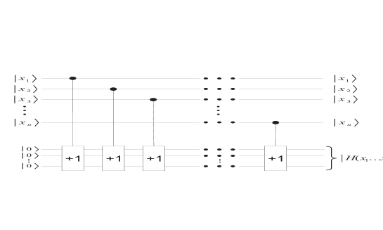
Figure 1: Network to compute the Hamming weight. $|x_{1}\cdots x_{n}\rangle|00\cdots 0\rangle\longrightarrow|x_{1}\cdots x_{n}\rangle|\mbox{H}(x_{1}\cdots x_{n})\rangle$.

Suppose Alice measures the Hamming weight of $|\Psi\rangle$ and obtains the result $|j\rangle$ (Bob will measure the same $j$ whenever he performs the same measurement). This state after the measurement is

$$\frac{1}{\sqrt{\binom{n}{j}}}\sum_{\mbox{H}(\mathbf{x})=j}\overset{a}{|\mathbf{x}\rangle}\overset{b}{|\mathbf{x}\rangle}$$

which can be thought of as a superposition of $\binom{n}{j}$ $n$-bit strings. (Of course, the measurement is not necessary, and the remainder of the algorithm could be controlled quantumly upon the value $j$.) Let $r=\lceil\log_{2}\binom{n}{j}\rceil$. Define a function $f$ on these $\binom{n}{j}$ strings that maps the ${n\choose j}$ strings of length $n$ with Hamming weight $j$ (in lexicographic order) to the integers from $0$ to ${n\choose j}-1$:

$$\begin{split}f(00\ldots 00\underset{j}{\underbrace{11\ldots 1}})&=00\ldots 0\\ f(00\ldots 10\underset{j-1}{\underbrace{11\ldots 1}})&=00\ldots 1\\ \hskip 28.45274pt\vdots&\\ f(\underset{j}{\underbrace{11\ldots 1}}00\ldots 0)&=\binom{n}{j}-1=m\\ &=\underset{n-r}{\underbrace{00\ldots 0}}\underset{r}{\underbrace{m}}.\end{split}$$

We can extend $f$ so that it defines a permutation of all $n$-bit strings. Then we have:

$$\begin{split}\frac{1}{\sqrt{\binom{n}{j}}}\sum_{\mbox{H}(x)=j}|\mathbf{x}\rangle|\mathbf{x}\rangle\overset{f}{\longrightarrow}&\sum_{\mbox{H}(x)=j}|f(\mathbf{x})\rangle|f(\mathbf{x})\rangle\\ &=\sum_{y=0}^{\binom{n}{j}-1}\underset{n-r}{\underbrace{|\mathbf{0}\rangle}}\underset{r}{\underbrace{|\mathbf{y}\rangle}}|\mathbf{0}\rangle|\mathbf{y}\rangle.\end{split}$$

If $\binom{n}{j}=2^{r}$, then ignoring the first $n-k$ bits on both sides gives us

$$\sum_{\mathbf{y}=0}^{2^{r}-1}|\mathbf{y}\rangle|\mathbf{y}\rangle$$

which is $r$ EPR-pairs, and the entanglement of $|\Psi\rangle$ has been concentrated.

However, in general, $\binom{n}{j}$ will not be a power of $2$. Let $k=\lfloor\log_{2}\binom{n}{j}\rfloor+1$. We describe a quantum network that will produce some number $0\leq l\leq k-1$ of EPR-pairs (we use this definition for $k$ in place of the previous definition for $r$ for convenience in describing a network that will behave the same whether or not $\binom{n}{j}$ is a power of 2). The expected number of EPR pairs will be at least $k-2$. We illustrate this for $n=3$ entangled pairs of qubits. Consider the binary representation $\binom{n}{j}=x_{2}x_{1}x_{0}=x_{2}\cdot 2^{2}+x_{1}\cdot 2^{1}+x_{0}\cdot 2^{0}$. We have

$$\sum_{\mathbf{y}=0}^{\binom{n}{j}-1}|\mathbf{y}\rangle|\mathbf{y}\rangle=\sum_{\mathbf{y}=0}^{x_{2}\cdot 2^{2}-1}|\mathbf{y}\rangle|\mathbf{y}\rangle+\sum_{\mathbf{y}=x_{2}\cdot 2^{2}}^{x_{2}\cdot 2^{2}+x_{1}\cdot 2^{1}-1}|\mathbf{y}\rangle|\mathbf{y}\rangle+\sum_{\mathbf{y}=x_{2}\cdot 2^{2}+x_{1}\cdot 2^{1}}^{x_{2}\cdot 2^{2}+x_{1}\cdot 2^{1}+x_{0}\cdot 2^{0}-1}|\mathbf{y}\rangle|\mathbf{y}\rangle.$$ (2)

Notice that if $x_{2}=1$ then the above sum includes $000\leq\mathbf{y}\leq 011$. These are included in $\sum_{\mathbf{y}=0}^{x_{2}\cdot 2^{2}-1}|\mathbf{y}\rangle|\mathbf{y}\rangle$ which is the first term on the right side of (2) (if $x_{2}=0$, then this term is empty). Similarly, if $x_{1}=1$ the sum includes $x_{2}00\leq\mathbf{y}\leq x_{2}01$ and if $x_{0}=1$ it includes $x_{2}x_{1}0\leq\mathbf{y}\leq x_{2}x_{1}1$. So we can write the sum (2) as follows:

$$\sum_{\mathbf{y}=0}^{\binom{n}{j}-1}|\mathbf{y}\rangle|\mathbf{y}\rangle=x_{2}\sum_{\mathbf{y}=000}^{011}|\mathbf{y}\rangle|\mathbf{y}\rangle+x_{1}\sum_{\mathbf{y}=x_{2}00}^{x_{2}01}|\mathbf{y}\rangle|\mathbf{y}\rangle+x_{0}\sum_{\mathbf{y}=x_{2}x_{1}0}^{x_{2}x_{1}0}|\mathbf{y}\rangle|\mathbf{y}\rangle.$$ (3)

In other words, for each $j$ such that $x_{j}=1$, we have the superposition of $2^{j}$ strings. Alice and Bob wish to project to one of these superpositions of $2^{j}$ strings, since that will provide them with $j$ EPR pairs.

The first term on the right side of (3) contains the strings $000$, $001$, $010$, $011$; all the strings beginning with a $0$. Suppose Alice performs a measurement of the qubit in the leftmost position (i.e. corresponding to $y_{2}$) of her share of the state $\sum_{\mathbf{y}=0}^{\binom{n}{j}-1}|\mathbf{y}\rangle|\mathbf{y}\rangle$ (Bob will obtain the same result whenever he performs the analogous measurement on his share). In addition, Alice also has the corresponding bit $x_{2}$ in a register containing the binary expansion of $\binom{n}{j}$. There are three cases to consider:

1. $y_{2}=0$ and $x_{2}=1$.

   In this case the joint state after the measurement is

   $$\sum_{\mathbf{y}=000}^{011}|\mathbf{y}\rangle|\mathbf{y}\rangle$$

   which is the first term on the right side of (3). Ignoring $|y_{2}\rangle$, this is 2 EPR pairs.

2. $y_{2}=0$ and $x_{2}=0$.

   The state after the measurement is

   $$x_{1}\sum_{\mathbf{y}=000}^{001}|\mathbf{y}\rangle|\mathbf{y}\rangle+x_{0}\sum_{\mathbf{y}=0x_{1}0}^{0x_{1}0}|\mathbf{y}\rangle|\mathbf{y}\rangle.$$

   Ignoring the leftmost qubit $|y_{2}\rangle$ this is equal to

   $$x_{1}\sum_{\mathbf{y}=00}^{01}|\mathbf{y}\rangle|\mathbf{y}\rangle+x_{0}\sum_{\mathbf{y}=x_{1}0}^{x_{1}0}|\mathbf{y}\rangle|\mathbf{y}\rangle.$$

3. $y_{2}=1$.

   In this case we know $x_{2}=1$. So the post-measurement state is

   $$x_{1}\sum_{\mathbf{y}=100}^{101}|\mathbf{y}\rangle|\mathbf{y}\rangle+x_{0}\sum_{\mathbf{y}=1x_{1}0}^{1x_{1}0}|\mathbf{y}\rangle|\mathbf{y}\rangle.$$

   Ignoring the leftmost qubit $|y_{2}\rangle$ this is equal to

   $$x_{1}\sum_{\mathbf{y}=00}^{01}|\mathbf{y}\rangle|\mathbf{y}\rangle+x_{0}\sum_{\mathbf{y}=x_{1}0}^{x_{1}0}|\mathbf{y}\rangle|\mathbf{y}\rangle.$$

If Alice’s measurement results in case 1, then the entanglement has been concentrated, and she makes no further measurements. Cases 2 and 3 both leave Alice and Bob with the state $x_{1}\sum_{\mathbf{y}=00}^{01}|\mathbf{y}\rangle|\mathbf{y}\rangle+x_{0}\sum_{\mathbf{y}=x_{1}0}^{x_{1}0}|\mathbf{y}\rangle|\mathbf{y}\rangle$. In either of these cases, Alice discards the leftmost qubit $|y_{2}\rangle$. She then repeats the measurement procedure, where this time the leftmost bits being measured are $y_{1}$ and $x_{1}$. The analogous three cases are considered again.

This time case 1 would result in the post measurement state $\sum_{\mathbf{y}=00}^{01}|\mathbf{y}\rangle|\mathbf{y}\rangle$. Ignoring the leftmost qubit $y_{1}$, this gives 1 EPR pair, and the procedure stops. Cases 2 and 3 both result in the post measurement state $x_{0}\sum_{\mathbf{y}=0}^{0}|\mathbf{y}\rangle|\mathbf{y}\rangle$, giving 0 EPR pairs.

It is easy to generalise this approach for $k=\lfloor\log_{2}\binom{n}{j}\rfloor+1$. Alice (or Bob) measures (locally) the qubits $y_{k-1},\ldots,y_{1}$, from “left-to-right”, at each step checking the value of the corresponding bit $x_{i}$ in the binary expansion of $\binom{n}{j}$. She does this until, at some iteration $l$ (where the first iteration is indexed 0), she finds $|y_{k-1-l}\rangle=|0\rangle$ and the corresponding bit $x_{k-1-l}=1$. When this occurs the procedure stops, having distilled $k-l-1$ EPR pairs.

Figure 2: Network to measure how many EPR pairs have been distilled.

A quantum network implementing the procedure is shown in Figure 2. Since the Hamming weight $j$ has been measured, $\binom{n}{j}$ can be efficiently computed. The binary representation of $\binom{n}{j}$ is encoded in a register $|x_{k-1}\ldots x_{0}\rangle$. The network makes use of an ancilla of size $k$, initially in the state $|1\rangle^{k}$. We refer to this ancilla as the “control ancilla”, and label its qubits of the by $|t_{i}\rangle$ for $0\leq i\leq k-1$. For each $i$, $|t_{i}\rangle$ is switched to $|0\rangle$ if both $|y_{i}\rangle=|0\rangle$ and $|x_{i}\rangle=|1\rangle$. This is achieved using a sequence of doubly controlled NOT gates in the first stage of the network, where the NOT is applied to the target qubit if the first control qubit is in state $|1\rangle$ and the second control qubit is in state $|0\rangle$. Another ancilla of size $O(\log(k-1))$, which we will call the “measurement ancilla” is initially in the state $|k-1\rangle$. In the second stage of the network, the value of the measurement ancilla is decremented by a sequence of controlled-[subtract 1] gates, controlled successively on each of the $|t_{i}\rangle$ in the control ancilla. The net effect of the first two stages of the network is to decrement the measurement ancilla by one for each pair $(|x_{i}\rangle,|y_{i}\rangle)$ until one such pair is found with $(|x_{i}\rangle=|1\rangle,|y_{i}\rangle=|0\rangle)$. After such a pair is encountered, the measurement ancilla is not decremented any more. In order to reverse the effect of any coupling that the network may have introduced between the primary register $|\mathbf{y}\rangle$ and the ancilla $|\mathbf{t}\rangle$, the same sequence of doubly controlled NOT gates that was used in the first stage of the network is applied again in the third stage.

The control ancilla has been reset to its initial state by the third stage of the network, and the register $|\mathbf{x}\rangle$ containing the binary expansion of $\binom{n}{j}$ is in a fixed computational basis state, since the value of $j$ was fixed by the Hamming weight measurement performed earlier. Ignoring the state the control ancilla and the register $|\bf{x}\rangle$, the joint state of Alice’s system $|\mathbf{y}\rangle$ and the measurement ancilla just before the final measurement is

$$x_{k-1}\sum_{y=0^{k}}^{01^{k-1}}|\mathbf{y}\rangle|k-1\rangle+x_{k-2}\sum_{y=x_{k-1}0^{k-1}}^{x_{k-1}01^{k-2}}|\mathbf{y}\rangle|k-2\rangle+\cdots+x_{0}\sum_{y=x_{k-1}\cdots x_{1}0}^{y=x_{k-1}\cdots x_{1}0}|\mathbf{y}\rangle|0\rangle.$$

The string $x_{k-1}x_{k-2}\ldots x_{k-l}$ correspond to the the leftmost $l$ bits in the binary representation of $\binom{n}{j}$. After the measurement of the control ancilla in the computational basis, the state is

$$\sum_{y=x_{k-1}x_{k-2}\ldots x_{k-l}0^{k-l}}^{x_{k-1}x_{k-2}\ldots x_{k-l}01^{k-l-1}}|\mathbf{y}\rangle|k-l-1\rangle$$

for some $0\leq l\leq k-1$. Ignoring the leftmost $l+1$ qubits, this is

$$\sum_{y=0^{k-l-1}}^{1^{k-l-1}}|\mathbf{y}\rangle|k-l-1\rangle.$$

Each ignoring their respective leftmost $l+1$ qubits, the joint Alice-Bob state is

$$\sum_{y=0^{k-l-1}}^{1^{k-l-1}}|\mathbf{y}\rangle|\mathbf{y}\rangle$$

which is $k-l-1$ EPR pairs. Note that the state of Alice’s ancilla (and Bob’s, if he performs the same measurement procedure on his share of the state) indicates the number of EPR pairs that have been distilled.

It should be noted that Alice and Bob can each carry out the above procedure locally, and they will obtain the same results. Alternatively, Alice could perform the Hamming weight computation locally and send the result to Bob. Alice and Bob would both perform the permutation $f$ by the method detailed in section 3). In the last stage of the procedure, either Alice or Bob could perform the computation to determine the number of EPR pairs that have been distilled, and send the result to the other.

It can be shown that given the superposition

$$\sum_{\mathbf{y}=0}^{\binom{n}{j}-1}|\mathbf{y}\rangle|\mathbf{y}\rangle$$

the average number of EPR-pairs produced using this approach is:

$$\sum_{i=1}^{\lfloor\log_{2}{\binom{n}{j}}\rfloor}x_{n-i}\frac{2^{i}}{\binom{n}{j}}\geq\lfloor\log_{2}{\binom{n}{j}}\rfloor-1=k-2.$$

3 Implementing the permutation $f$

The key step in the entanglement concentration protocol is the permutation $f$. We need to know how to implement this function. Recall that we start with a superposition of $\binom{n}{j}$ strings $\mathbf{x}$, each having $j$ $1s$ and $n-j$ $0s$. We want $f$ to impose a lexicographic ordering on these strings.

Consider the following:

$$\begin{split}0\hskip 2.84526pt0\hskip 2.84526pt\ldots\hskip 2.84526pt0\hskip 8.53581pt&\overset{f^{-1}}{\longrightarrow}\hskip 8.53581pt0\hskip 2.84526pt0\hskip 2.84526pt\ldots\hskip 2.84526pt0\hskip 2.84526pt0\hskip 2.84526pt\underset{j}{\underbrace{1\hskip 2.84526pt1\hskip 2.84526pt\ldots\hskip 2.84526pt1}}\\ 0\hskip 2.84526pt0\hskip 2.84526pt\ldots\hskip 2.84526pt1\hskip 8.53581pt&\overset{f^{-1}}{\longrightarrow}\hskip 8.53581pt0\hskip 2.84526pt0\hskip 2.84526pt\ldots\hskip 2.84526pt1\hskip 2.84526pt0\hskip 2.84526pt\underset{j-1}{\underbrace{1\hskip 2.84526pt1\hskip 2.84526pt\ldots\hskip 2.84526pt1}}\\ &\hskip 14.22636pt\vdots\\ \binom{n-1}{j}-1\hskip 8.53581pt&\overset{f^{-1}}{\longrightarrow}\hskip 8.53581pt0\hskip 2.84526pt\underset{j}{\underbrace{1\hskip 2.84526pt1\hskip 2.84526pt\ldots\hskip 2.84526pt1}}\hskip 2.84526pt0\hskip 2.84526pt0\hskip 2.84526pt\ldots\hskip 2.84526pt0\\ \binom{n-1}{j}\hskip 8.53581pt&\overset{f^{-1}}{\longrightarrow}\hskip 8.53581pt1\hskip 2.84526pt0\hskip 2.84526pt\ldots\hskip 2.84526pt0\hskip 2.84526pt\underset{j-1}{\underbrace{1\hskip 2.84526pt1\hskip 2.84526pt\ldots\hskip 2.84526pt1}}\\ &\hskip 14.22636pt\vdots\\ \binom{n}{j}-1\hskip 8.53581pt&\overset{f^{-1}}{\longrightarrow}\hskip 8.53581pt\underset{j}{\underbrace{1\hskip 2.84526pt1\hskip 2.84526pt\ldots\hskip 2.84526pt1}}\hskip 2.84526pt0\hskip 2.84526pt0\hskip 2.84526pt\ldots\hskip 2.84526pt0.\end{split}$$

The first $\binom{n-1}{j}$ strings have a $0$ in the first bit position, and the remaining strings have a $1$ in the first bit position. Define $[\mathbf{y}]_{n,j}$ to be the $\mathbf{y}^{th}$ largest string (treating the string as an integer represented in binary) of length $n$ with Hamming weight $j$. Using this notation, the method for implementing $f$ is captured by the following recurrence:

$$\begin{split}[\mathbf{y}]_{n,j}&=0[\mathbf{y}]_{n-1,j}\hskip 79.6678pt\mbox{ if }0\leq\mathbf{y}<\binom{n-1}{j}\\ &=1\left[\mathbf{y}-\binom{n-1}{j}\right]_{n-1,j-1}\mbox{ if }\binom{n-1}{j}\leq\mathbf{y}<\binom{n}{j}.\end{split}$$ (4)

We describe how the permutation $f^{-1}$ can be implemented on a quantum computer. Let $[\mathbf{y}]_{n,j}=b_{1}b_{2}\ldots b_{n}$. Then start with a string between $00\ldots 0$ and $\binom{n}{j}-1$, and ancilla holding the values $n$, $j$, and a space for the output strings $f^{-1}(\mathbf{y})$:

$$|\mathbf{y}\rangle|n\rangle|j\rangle|00\ldots 0\rangle.$$

Apply an operator $T$ which performs the following mapping:

$$\begin{split}|\mathbf{y}\rangle|n\rangle|j\rangle|00\ldots 0\rangle&\overset{T}{\longrightarrow}|\mathbf{y}\rangle|n\rangle|j\rangle|00\ldots 0\rangle\hskip 14.22636pt\mbox{ if }\hskip 5.69054pt0\leq\mathbf{y}<\binom{n-1}{j}\\ &\overset{T}{\longrightarrow}|\mathbf{y}\rangle|n\rangle|j\rangle|10\ldots 0\rangle\hskip 14.22636pt\mbox{ if }\hskip 5.69054pt\binom{n-1}{j}\leq\mathbf{y}<\binom{n}{j}.\end{split}$$

The result is:

$$|\mathbf{y}\rangle|n\rangle|j\rangle|00\ldots 0\rangle\overset{T}{\longrightarrow}|\mathbf{y}\rangle|n\rangle|j\rangle|b_{1}0\ldots 0\rangle$$

for some $b_{1}\in\{0,1\}$. Then perform the following subtraction operation $S$, controlled quantumly on the value of $b_{1}$:

$$\begin{split}|\mathbf{y}\rangle|n\rangle|j\rangle&\overset{S}{\longrightarrow}|\mathbf{y}\rangle|n-1\rangle|j\rangle\hskip 93.89409pt\mbox{ if }\hskip 5.69054ptb_{1}=0\\ &\overset{S}{\longrightarrow}|\mathbf{y}-\binom{n-1}{j}\rangle|n-1\rangle|j-1\rangle\hskip 14.22636pt\mbox{ if }\hskip 5.69054ptb_{1}=1.\end{split}$$

Then repeat $T$ and $S$, this time on only the right-most $n-1$ bits of the registers $|y\rangle$ and $|b_{1}0..0\rangle$. Applying $T$ and $S$ in this way, a total of $n$ times, realises the recurrence (4), and gives us an implementation of $f^{-1}$:

$$|\mathbf{y}\rangle\overset{f^{-1}}{\longrightarrow}|[{\mathbf{y}}]_{n,j}\rangle$$

and thus the same network maps

$$\sum_{\mathbf{y}=\mathbf{0}}^{\binom{n}{j}-1}|\mathbf{y}\rangle\overset{f^{-1}}{\longrightarrow}\sum_{H(\mathbf{x})=j}|\mathbf{x}\rangle.$$

The permutation $f$ is realised simply by running this procedure backwards.

4 An algorithm for entanglement concentration

We now have the tools to state an algorithm for implementing the entanglement concentration protocol described in section 4.1. The algorithm is the following:

1. Begin with the state $|\Psi\rangle=(\alpha|00\rangle+\beta|11\rangle)^{n}$.

2. Alice and Bob each perform a Hamming-weight measurement on their half of $|\Psi\rangle$, obtaining the same result $|j\rangle$.

3. Alice and Bob each perform the permutation $f$ on the resulting superposition.

4. Alice and Bob each use the network of Figure 2 to determine how many EPR pairs they share.

5. The result is some known number of perfect EPR pairs. For a particular $j$, the expected number is between $k-2$ and $k-1$ where $k=\lfloor\log_{2}{n\choose j}\rfloor+1$.

Each of the above steps have been detailed in the preceding sections, and so we have a complete description of the implementation. Since the probability of measuring $|j\rangle$ in step 2 is

$$|\alpha^{2}|^{n-j}\left(1-|\alpha^{2}|\right)^{j}{n\choose j},$$

the expected number of EPR pairs is at least

$$\sum_{j=0}^{n}|\alpha^{2}|^{n-j}\left(1-|\alpha^{2}|\right)^{j}{n\choose j}(\lfloor\log_{2}{n\choose j}\rfloor-1)$$

and comparing to equation (1) shows that we get at least

$$nH(|\alpha^{2}|)-O(\log n)$$

EPR pairs on average. Note that the theoretical maximum is $nH(|\alpha^{2}|)$.

References

• [1]
• [BBCJPW93] Charles Bennett, Gilles Brassard, Claude Crepeau, Richard Josza, Asher Peres, William Wootters. “Teleporting an Unknown Quantum State via Dual Classical and Einstein-Podolsky-Rosen Channels” Physical Review Letters, 70, 1895-1898, 1993.
• [BBHT98] Michel Boyer, Gilles Brassard, Peter Høyer, Alain Tapp. “Tight bounds on quantum searching” Fortschritte der Physik, 56(5-5), 493-505, 1998. On the quant-ph archive, report no. 9605034.
• [BBPS95] Charles Bennett, Herbert Bernstein, Sandu Popescu, Benjamin Schumacher. “Concentrating Partial Entanglement by Local Operations” Phys. Rev. A, 53, 2046 (1996). On the quant-ph archive, report no. 9511030.
• [BCW98] Harry Buhrman, Richard Cleve, Avi Wigderson. “Quantum vs. Classical Communication and Computation” in Proceedings of the 30th Annual ACM Symposium on Theory of Computing (STOC98), pages 63-68. On the quant-ph archive, report no. 9705033.
• [BH97] Gilles Brassard, Peter Høyer. “An exact quantum polynomial-time algorithm for Simon’s problem” Proceedings of fifth Israeli Symposium on Theory of Computing and Systems, 12-23. IEEE Computer Society Press, 1997.
• [BHMT00] Gilles Brassard, Peter Høyer, Michele Mosca, Alain Tapp. “Quantum Amplitude Amplification and Estimation”, to appear in Quantum Computation and Quantum Information Science, AMS Contemporary Math Series, 2000.
• [BHT98] Gilles Brassard, Peter Høyer, Alain Tapp. “Quantum Counting” in Proceedings of the ICALP’98 Lecture notes in Computer Science 1443, 1820-831, 1998. On the quant-ph archive, report no. 9805082.
• [CEMM98] Richard Cleve, Artur Ekert, Chiara Macchiavello, Michele Mosca. “Quantum Algorithms Revisited” Proceedings of the Royal Society of London A, 454, 339-354, 1998. On the quant-ph archive, report no. 9708016.
• [Deu85] David Deutsch. “Quantum theory, the Church-Turing principle and the universal quantum computer” Proceedings of the Royal Society of London A, 400: 97-117, 1985.
• [Eke91] Artur Ekert, “Quantum cryptography based on Bell’s theorem”, Physical Review Letters, 67(6, 5), 1991.
• [EPR35] A. Einstein, B. Podolsky, and N. Rosen. “Can quantum-mechanical description of reality be considered complete?” Physical Review 47, 777-780 (1935).
• [Fey82] Richard Feynman. “Simulating Physics with Computers” International Journal of Thoertical Physics, 21(6,7), 467-488, 1982.
• [Gro96] Lov Grover. “A fast quantum mechanical algorithm for database search” Proceedings of the 28th Annual ACM Symposium on the Theory of Computing (STOC’96), 212-219, Philadelphia, Pennsylvania, 1996.
• [Mos98] M. Mosca, “Quantum searching and counting by eigenvector analysis”, in Proceedings of Randomized Algorithms, Workshop of MFCS 98, Brno, Czech Republic, (1998)
• [Mos99] Michele Mosca. “Quantum Computer Algorithms”. D.Phil. Dissertation. Wolfson College, University of Oxford, 1999.
• [Raz99] Ran Raz. ”Exponential Separation of Quantum and Classical Communication Complexity”. Proceedings of the 31st Annual ACM Symposium on the Theory of Computing (STOC’99), 358-367, 1999.
• [Sho94] Peter Shor. “Algorithms for Quantum Computation: Discrete Logarithms and Factoring” Proceedings of the 35th Annual Symposium on Foundations of Computer Science, 124-134, 1994.