Stochastic Theory of Relativistic Particles Moving in a Quantum Field: II. Scalar Abraham-Lorentz-Dirac-Langevin Equation, Radiation Reaction and Vacuum Fluctuations
Abstract
We apply the open systems concept and the influence functional formalism introduced in Paper I to establish a stochastic theory of relativistic moving spinless particles in a quantum scalar field. The stochastic regime resting between the quantum and semi-classical captures the statistical mechanical attributes of the full theory. Applying the particle-centric world-line quantization formulation to the quantum field theory of scalar QED we derive a time-dependent (scalar) Abraham-Lorentz-Dirac (ALD) equation and show that it is the correct semiclassical limit for nonlinear particle-field systems without the need of making the dipole or non-relativistic approximations. Progressing to the stochastic regime, we derive multiparticle time-dependent ALD-Langevin equations for nonlinearly coupled particle-field systems. With these equations we show how to address time-dependent dissipation/noise/renormalization in the semiclassical and stochastic limits of QED. We clarify the relation of radiation reaction, quantum dissipation and vacuum fluctuations and the role that initial conditions may play in producing non-Lorentz invariant noise. We emphasize the fundamental role of decoherence in reaching the semiclassical limit, which also suggests the correct way to think about the issues of runaway solutions and preacceleration from the presence of third derivative terms in the ALD equation. We show that the semiclassical self-consistent solutions obtained in this way are “paradox” and pathology free both technically and conceptually. This self-consistent treatment serves as a new platform for investigations into problems related to relativistic moving charges.
I Introduction
This is the second in a series of three papers [1, 2] exploring the regime of stochastic behavior manifested by relativistic particles moving through quantum fields. This series highlights the intimate connections between backreaction, dissipation, noise, and correlation, focusing on the necessity (and the consequences) of a self-consistent treatment of nonlinearly interacting quantum dynamical particle-field systems.
In Paper I [1], we have set up the basic framework built on the influence functional and worldline quantization formalism. In this paper we apply the results obtained there to spinless relativistic moving particles in a quantum scalar field. The interaction is chosen to be the scalar analog of QED coupling so that we can avoid the complications of photon polarizations and gauge invariance in an electromagnetic field. The results here should describe correctly particle motion when spin and photon polarization are unimportant, and when the particle is sufficiently decohered such that its quantum fluctuations effectively produce stochastic dynamics.
The main results of this investigation are
-
1.
First principle derivation of a time-dependent (modified) Abraham-Lorentz-Dirac (ALD) equation as the consistent semiclassical limit for nonlinear particle-scalar-field systems without making the dipole or non-relativistic approximations.
-
2.
Consistent resolution of the paradoxes of the ALD equations, including the problems of runaway and acausal (e.g. pre-accelerating) solutions, and other “pathologies”. We show how the non-Markovian nature of the quantum particle open-system enforces causality in the equations of motion. We also discuss the crucial conceptual role that decoherence plays in understanding these problems.
-
3.
Derivation of multiparticle Abraham-Lorentz-Dirac-Langevin (ALDL) equations describing the quantum stochastic dynamics of relativistic particles. The familiar classical Abraham-Lorentz-Dirac (ALD) equation is reached as its noise-averaged form. The stochastic regime, characterized by balanced noise and dissipation, plays a crucial role in bridging the gap between quantum and (emergent) classical behaviors. The N-particle-irreducible (NPI) and master effective action [3, 4, 5, 6] provide a route for generalizing our treatment to the self-consistent inclusion of higher order quantum corrections.
We divide our introduction into three parts: First, a discussion of the pathologies and paradoxes of the ALD equation from the conventional approach and our suggested cures based on proper treatment of causal and non-Markovian behavior and self-consistent backreaction. Second, misconceptions in the relation between radiation reaction, quantum dissipation and vacuum fluctuations and the misplaced nature and role of fluctuation-dissipation relations. Finally we give a brief summary of previous work and describe their shortcomings which justify a new approach as detailed here.
A Pathologies, Paradoxes, Remedies and Resolutions
The classical theory of moving charges interacting with a classical electromagnetic field has controversial difficulties associated with backreaction [7, 8]. The generally accepted classical equation of motion in a covariant form for charged, spinless point particles, including radiation-reaction, is the Abraham-Lorentz-Dirac (ALD) equation [9]:
| (1) |
The timescale determines the relative importance of the radiation-reaction term. For electrons, secs, which is roughly the time it takes light to cross the electron classical radius m. The ALD equation has been derived in a variety of ways, often involving some regularization procedure that renormalizes the particle’s mass [10]. Feynman and Wheeler have derived this result from their “Absorber” theory which symmetrically treats both advanced and retarded radiation on the same footing [11].
The ALD equation has strange features, whose status are still debated. Because it is a third order differential equation, it requires the specification of extra initial data (e.g. the initial acceleration) in addition to the usual position and velocity required by first order Hamiltonian systems. This leads to the existence of runaway solutions. Physical (e.g. non-runaway) solutions may be enforced by transforming (1) to a second order integral equation with boundary condition such that the final energy of the particle is finite and consistent with the total work done on it by external forces. But the removal of runaway solutions comes at a price, because solutions to the integral equation exhibit the acausal phenomena of pre-acceleration on timescales This is the source of lingering questions on whether the classical theory of point particles and fields is causal***Another mystery of the ALD equation is the problem of the constant force solution, where the charge uniformly accelerates without radiation reaction, despite it being well-established that there is radiation. This is a case where local notions of energy must be carefully considered in theories with local interactions (between point particles) mediated by fields [12, 13]. The classical resolution of this problem involves recognizing that one must consider all parts of the total particle-field system with regard to energy conservation: particle energy, radiation energy, and non-radiant field energy such as resides in the so-called acceleration (or Shott) fields [13]..
B Radiation Reaction and Vacuum Fluctuations
The stochastic regime is characterized by competition between quantum and statistical processes: particularly, quantum correlations versus decoherence, and fluctuations versus dissipation. The close association of vacuum fluctuations with radiation-reaction is well-known, but the precise relationship between them requires clarification. It is commonly asserted that vacuum fluctuations (VF) are balanced by radiation reaction (RR) through a fluctuation-dissipation relation (FDR). This can be misleading. Radiation reaction is a classical process (i.e., ) while vacuum fluctuations are quantum in nature. A counter-example to the claim that there is a direct link between RR and VF is the uniformly accelerated charged particle (UAP) for which the classical radiation reaction force vanishes, but vacuum fluctuations do not. However, at the stochastic level variations in the radiation reaction force away from the classical averaged value exist – it is this quantum dissipation effect which is related to vacuum fluctuations by a FDR.
From discussions in Paper I we see how decoherence enters in the quantum to classical transition. Under reasonable physical conditions [18] the influence action or decoherence functional is dominated by the classical solution (via the stationary phase approximation). Also from the ‘non-Markovian’ fluctuation-dissipation relations found in Paper I, we see that the relationship between noise and dissipation is extremely complicated. Here too, decoherence plays a role in the emergence of the usual type fluctuation-dissipation kernel, just as it plays a role in the emergence of classicality. When there is sufficient decoherence, the FDR kernel (see Eq. (5.23) in Paper I) is dominated by the self-consistent semiclassical (decoherent) trajectories. An approximate, linear FDR relation may be obtained (see Eq. (5.24) in Paper I) except that the kernel is self-consistently determined in terms of the average (mean) system history, and the FDR describes the balance of fluctuations and dissipation about those mean trajectories.
These observations have important ramifications on the appropriateness of assigning a FDR for radiation reaction and vacuum fluctuations. Ordinary (e.g. classical) radiation reaction is consistent with the mean particle trajectories determined by including the backreaction force from the field. But at the classical level, there are no fluctuations, and hence no fluctuation-dissipation relation. Even regarding radiation reaction as a ‘damping’ mechanism is misleading– it is not ‘dissipation’ in the true statistical mechanical sense. Unlike a particle moving in some viscous medium whose velocity is damped, radiation reaction generally vanishes for inertial (e.g. constant velocity) particles moving in vacuum fields (e.g. QED). Furthermore, radiation reaction can both ‘damp’ and anti-‘damp’ particle motion, though the average effect is usually a damping one. On the other hand, we show that the fluctuations around the mean-trajectory are damped, as described by a FDR. At the quantum stochastic level as discussed here, quantum dissipation effect results from the changes in the radiation reaction force that are associated with fluctuations in the particle trajectory around the mean, and therefore it is not the same force as the classical (i.e. average) radiation reaction force. Only these quantum processes obey a FDR. This is a subtle noteworthy point.
C Prior work in relation to ours
-
1.
There are many works on nonrelativistic quantum (and semiclassical) radiation reaction (for atoms as well as charges moving in quantum fields) including those by Rohrlich, Moniz-Sharp, Cohen-Tannoudji et. al., Milonni, and others [8, 13, 19, 20, 21]. Kampen, Moniz, Sharp, and others [14] suggested that the problems of causality and runaways can be resolved in both classical and quantum theory by considering extended charge models. However, this approach, while quite interesting, misses the point that point particles (like local quantum field theories) obey a good low energy effective theory in their own right. While it is true that extended objects can cure infinities (e.g., extended charge models, string theory), it is nonetheless important to recognize that at sufficiently low energy QED as an effective field theory is ‘consistent’ without recourse to its high-energy limit. Wilson, Weinberg and others [22] have shown how effective theory description is sufficient to understand low energy physics because complicated, and often irrelevant, high energy details of the fine structure are not being probed at the physical energy scales of interest. The effective theory approach has also provided a new perspective on the physical meaning of renormalization and the source of divergences, showing why nonrenormalizable interactions are not a disaster, why the apparent large shift in bare-parameters resulting from divergent loop diagrams (i.e. renormalization) doesn’t invalidate perturbation theory, and clarifying how and when high-energy structure does effect low-energy physics. Therefore one should not need to invoke extended charge theory to understand low energy particle dynamics.
Our work is a relativistic treatment which includes causal Non-Markovian behavior and self-consistent backreaction. We think this is a better approach even in a nonrelativistic context because the regularized relativistic theory never ‘breaks down’. In our approach we adopt the ideas and methods of effective field theory with proper treatment of backreaction to account for the effects of high-energy (short-distance) structure on low-energy behavior, and to demonstrate the self-consistency of the semiclassical particle dynamics. We consider the consequences of coarse-graining the irrelevant (environmental) degrees of freedom, and the nature of vacuum fluctuations and quantum dissipation in the radiation reaction problem. We emphasize the crucial role of decoherence due to noise in resolving the pathologies and paradoxes, and in seeing how causal QED leads to a (short-time modified) causal ALD semiclassical limit.
-
2.
By examining the time-dependence of operator canonical commutation relations Milonni showed the necessity of electromagnetic field vacuum fluctuations for radiating nonrelativistic charges [21]. The conservation of the canonical commutation relations is a fundamental requirement of the quantum theory. Yet, if a quantum particle is coupled to a classical electromagnetic field, radiative losses (dissipation) lead to a contraction in “phase-space” for the expected values of the particle position and momentum, which violates the commutation relations. It is the vacuum field that balances the dissipation effect, preserving the commutation relations as a consequence of a fluctuation-dissipation relation (FDR). The particle-centric worldline framework allows us to consider similar issues for relativistic particles. Interestingly, our covariant framework shows how quantum fluctuations (manifesting as noise) appear in both the time and space coordinates of a particle. This is not surprising since relativity requires that a physical particle satisfies and therefore any variation in spatial velocities must be balanced by a change in keeping the particle “on-shell”.
-
3.
The derivation and use of quantum Langevin equations (QLE’s) to describe fluctuations of a system in contact with a quantum environment has a long history. Typically, QLE’s are assumed to describe fluctuations in the linear response regime for a system around equilibrium, but its validity does not need be so restrictive. Nonequilibrium conditions can be treated with the Feynman-Vernon influence functional. Caldeira and Leggett’s study of quantum Brownian motion (QBM) has led to an extensive literature [23], particularly in regard to decoherence issues[24]. Barone and Caldeira [25] have applied this method to the question of whether nonrelativistic, dipole coupled electrons decohere in a quantum electromagnetic field. An advantage of Barone and Caldeira’s work is that it is not limited to initially factorized states; they use the preparation function method which allows the inclusion of initial particle field correlations. Despite this, Romero and Paz have pointed out that the preparation function method still suffers from an (implicit) unphysical depiction of instantaneous measurement characterizing the initial state preparation [26].
-
4.
Ford, Lewis, and O’Connell have extensively discussed the electromagnetic field as a thermal bath in the linear, dipole coupled regime [17], and pioneered the application of QLE’s to nonrelativistic particle motion in QED. They have detailed the conditions for causality in the thermodynamic, equilibrium limit described by the late-time linear quantum Langevin equation. A crucial point of their analysis is that particle motion can be (depending on the cutoff of the field spectral density) runaway free and causal in the late-time limit [27]. In [28], they suggest a form of the equations of motion that gives fluctuations without dissipation for a free electron, but this result is special to the particular choice of a field cutoff made by the authors, namely, one implying that the bare mass of the particle exactly vanishes. When one does not assume a special value for the cutoff one generally does find both fluctuations and dissipation, though Ford and Lewis’s counter-example shows how careful one must be in handling FDRs. Another counter-example against making hasty generalizations is the vanishing of the averaged (classical) radiation reaction for uniformly accelerated particles despite quantum fluctuations that make the (suitably coarse-grained) trajectories stochastic.
We do agree with the result that the particle motion is only causal and consistent when the field cutoff is below a certain critical value†††A noted example is in Caldeira and Leggett’s original work [16]. Their master equation governs a reduced density matrix which is not positive definite because they choose an (infinite) cutoff greater than the inverse temperature (see Hu, Paz, and Zhang [23] for details). (determined from the particles classical radius), but we find no compelling justification for the claim that the cutoff should take exactly that special value.
It is certainly interesting that with the special field-cutoff chosen by Ford and O’Connell higher time-derivatives vanish from the equations of motion. However, even without such a specially chosen cutoff, the influence of higher derivative terms are strongly suppressed at low energies. On this issue we take the effective theory point of view which emphasizes the generic insensitivity of low-energy phenomena to unobserved high-energy structures. Since higher-time derivatives in the equations of motion do not (necessarily) violate causality, there is no reason to rule them out. It is perhaps instructive to review the meaning of renormalizable field theories in the light of effective theories. Effective theories generically have higher derivative interactions that are again strongly suppressed at low energies. What makes renormalizable terms special is that these are the interactions that remain relevant (or marginal) at low energies, while non-renormalizable terms (such as higher derivative terms) are exponentially suppressed, hence, it is no longer believed that non-renormalizable terms are fundamentally excluded so long as one recognizes that physical theories are mostly effective theories. Since QED is certainly an effective theory, these observations (together with the suppression of the higher time-derivative terms) weaken the argument that the special cutoff theory of FOL is fundamental. Ford and O’Connell also propose a relativistic generalization of their modified equations of motion for the average trajectory derived from the nonrelativistic QLE [29]. Our derivation of the stochastic limit from a relativistic quantum mechanics (i.e. worldline formulation) and field theory goes well beyond this by allowing the treatment of fully quantum relativistic processes, and by deriving a relativistic Langevin equation.
-
5.
A perturbative expansion of the ALD equation up to order has been derived from QED field theory by Krivitskii and Tsytovich [30], including the additional forces arising from particle spin. Their work shows that the ALD equation may also be understood from field theory, but the authors have not addressed the role of fluctuations, correlation, decoherence, time-dependent renormalization, nor self-consistent backreaction. Our derivation yields the full ALD equation (all orders in for the perturbation expansion employed by [30]) through the loop (semiclassical) expansion; this method automatically includes all tree-level diagrammatic effects.
-
6.
Low [31] showed that runaway solutions apparently do not occur in spin 1/2 QED. But Low does not derive the ALD equation, nor address the semiclassical/stochastic limit. We also emphasize, again, that it does not, and should not, matter whether particles are spin 1/2, spin 0, or have some other internal structure in regard to the causality of the low energy effective theory for center of mass particle motion.
-
7.
Using the influence functional, Diósi [32] derives a Markovian master equation in non-relativistic quantum mechanics. In contrast, it is our intent to emphasize the non-Markovian and nonequilibrium regimes with special attention paid to self-consistency. The work of [32] differs from ours in the treatment of the influence functional as a functional of particle trajectories in the relativistic worldline quantization framework. Ford has considered the loss of electron coherence from vacuum fluctuation induced noise with the same noise kernel that we employ [33]. However, his application concerns the case of fixed or predetermined trajectories.
D Organization
In Section II we obtain the influence functional (IF) for spinless relativistic particles. We then define the stochastic effective action for this model, using our results from Paper I, and use it to derive nonlinear integral Langevin equations for multiparticle spacetime motion. In Section III we consider the single particle case. We derive the (scalar-field) Abraham-Lorentz-Dirac (ALD) equation as the self-consistent semiclassical limit, and show how this limit emerges free of all pathologies. In Section IV we derive a Langevin equation for the stochastic fluctuations of the particle spacetime coordinates about the semiclassical limit for both the one particle and multiparticle cases. We also show how a stochastic version of the Ward-Takahashi identities preserves the mass-shell constraint. In Section V, we give a simple example of these equations for a single free particle in a scalar field. We find that in this particular case the quantum field induced noise vanishes, though this result is special to the overly-simple scalar field, and does not hold for the electromagnetic field [2]. In the final section, we summarize our main results and mention areas of applications, of both theoretical and practical interest.
II Spinless relativistic particles moving in a scalar field
A The model
Relativistic quantum theories are usually focused primarily on quantized fields, the notion of particles following trajectories is somewhat secondary. As explained in Paper I [1], we employ a “hybrid” model in which the environment is a field, but the system is the collection of particle spacetime coordinates (i.e., worldlines) where indicates the particle coordinate, with worldline parameter charge and mass The free particle action is
| (2) |
From follow the relativistic equations of motion:
| (3) |
For generality, we include a possible background potential in addition to the quantum scalar field environment. The scalar current is
| (4) |
where
| (5) |
In Paper III [2], we treat a vector current coupled to the electromagnetic vector potential . In both cases we assume spinless particles. The inclusion of spin or color is important to making full use of these methods in QED and QCD.
In the full quantum theory reparametrization invariance of the relativistic particle plays a crucial role, and the particle-field interaction must respect this symmetry. When dealing with the path integral for the quantized particle worldline, a quadratic form of the action is often more convenient than the square-root action in (2). The worldline quantum theory is a gauge theory because of the constraint that follows from reparametrization invariance under making this perhaps the simplest physical example of a generally covariant theory. (We may therefore view this work as a toy model for general relativity, and for string theory, in the semiclassical and stochastic regime.) The path integral must therefore be gauge-fixed to prevent summing over gauge-equivalent histories. In [34] we treat the full quantum theory, in detail, and derive the “worldline influence functional” after fixing the gauge to the so-called proper-time gauge. This give the worldline path integral in terms of a sum over particle trajectories satisfying but where the path integral still involves an integration over possible (the range of this integration depends on the boundary conditions for the problem at hand). However, applying the semiclassical (i.e., loop) expansion in [34] we find that the trajectory gives the stationary phase solution; hence, the semiclassical limit‡‡‡Note however that in the stochastic limit there can potentially be fluctuations in the value of the constraint. corresponds to setting In the following we will therefore assume the constraint or even when we are discussing the semiclassical limit for trajectories. We show that this is self-consistent in that it is preserved by the equations of motion including noise-induced fluctuations in the particle trajectory. Since we are addressing the semiclassical/stochastic limit in this paper there is no need to adopt the quadratic form of action for a relativistic particle; it is adequate, and it turns out to be simpler in this paper, to just work with the scalar functions defined in (5), and the square-root form of the relativistic particle action in (2).
While we emphasize the microscopic quantum origins, we might also view our model in analogy to the treatment of quantum fields in curved spacetime. There, one takes the gravitational field (spacetime) as a classical system coupled to quantum fields. One important class of problems is then the backreaction of quantum fields on the classical spacetime. The backreaction of their mean yields the semiclassical Einstein equation which forms the basis of semiclassical gravity. The inclusion of fluctuations of the stress-energy of the quantum fields and the induced metric fluctuations yields the Einstein-Langevin equations [35] which forms the basis of this stochastic semiclassical gravity [36]. In our work here, the particle coordinates are analogous to the gravitational field (metric tensor). Whereas the Einstein-Langevin equations have not been derived from first principles for the lack of a quantum theory of gravity, we shall take advantage of the existence of a full quantum theory of particles and fields to examine how, and when, a regime of stochastic behavior emerges.
B The influence functional and stochastic effective action
The interaction between the particles and a scalar field is given by the monopole coupling term
| (6) | ||||
| (7) |
This is the general type of interaction treated in Paper I. In the second line we have used the expression for the current (4). The expression for the influence functional (Eq. (3.16) of Paper I) [37] is,
| (8) | ||||
| (9) |
where
| (10) | ||||
| (11) |
and are a pair of particle histories. and are the scalar field retarded and Hadamard Green’s functions, respectively. Substitution of (4) then gives the multiparticle influence functional
| (12) | ||||
| (13) | ||||
| (14) | ||||
| (15) | ||||
| (16) | ||||
| (17) |
where The influence functional may be expressed more compactly by using a matrix notation where , giving
| (18) | ||||
| (19) | ||||
| (20) | ||||
| (21) |
The superscript denotes the transpose of the column vector In (20), and below, we leave the sum and integrations implicit for brevity. The matrices are given by
| (22) | ||||
| (25) |
and
| (26) | ||||
| (29) |
In Eq. (21), we have defined the influence action . are the scalar-field Hadamard/Retarded Green’s functions evaluated at various combinations of spacetime points
The stochastic effective action is defined by (see [1])
| (30) | ||||
| (31) | ||||
| (32) |
where
| (33) |
and is a (classical) stochastic field (see Section 3 of Paper I) evaluated at the spacetime position of the th particle. The stochastic field has vanishing mean and autocorrelation function given by
| (34) |
Hence, statistics encodes those of the quantum field .
The stochastic effective action provides an efficient means for deriving self-consistent Langevin equations that describe the effects of quantum fluctuations as stochastic particle motion for sufficiently decohered trajectories (for justification in using in this way see Paper I).
C Langevin integrodifferential equations of motion
Deriving a specific Langevin equation from the general formalism of Paper I requires evaluating the cumulants defined in Eq. (4.11) of [1]. Because the multiparticle case involves a straightforward generalization, we begin with the single particle theory. The noise cumulants are then defined as
| (35) |
with given in (21). The superscript indicates that these are cumulants for an expansion of with respect to the stochastic variables
We define new variables where and and
| (36) |
Then the influence action has the form
| (37) |
where
| (38) | ||||
| (41) |
and
| (42) | ||||
| (45) |
The lowest order cumulant in the Langevin equation, is found by evaluating , and then setting There are two kinds of terms that arise: those where acts on and those where it acts on For linear theories, R,H is not a function of the dynamical variables, but is instead (at most) a function of some predetermined kinematical variables that a priori specify the trajectory. Hence, there is no contribution from . For the terms, setting collapses the matrices (38 and 42) to one term each: only the term of and the term of survive. But, setting gives and since the term of is proportional to two factors of it also vanishes. When acts on only the terms survive (because it is the only term not proportional to a factor of For similar reasons, the only contributing element of is also its term. To evaluate we note
| (46) |
After a little algebra, we are left with
| (47) |
where the derivative only acts on the and not the argument, in The same algebra in evaluating the term shows that all the factors cancel, and therefore does not contribute to the first cumulant at all. Because the imaginary part of does not contribute to the first cumulant, the equations of motion of the mean-trajectory are explicitly real, which is an important consequence of using an initial value formulation like the influence functional (or closed-time-path) method.
The first cumulant, describing radiation reaction, is therefore given by
| (48) | |||
| (49) | |||
| (50) |
This expression is explicitly causal both because the proper-time integration is only over values , and because of the explicit occurrence of the retarded Green’s function. Contrary to common perception, the radiation reaction force given by is not necessarily dissipative in nature. For instance, we shall see that vanishes for uniformly accelerated motion, despite the presence of radiation from a uniformly accelerating charge. In other circumstances, may actually provide an anti-damping force for some portions of the particle trajectory.
Hence, radiation reaction is not a purely dissipative, or damping, process. The relationship of radiation reaction to vacuum fluctuations is also not simply given by a fluctuation-dissipation relation§§§Fluctuation-dissipation related arguments have been frequently invoked for radiation reaction problems, but these instances generally entail linearizing (say, making the dipole approximation), and/or the presence of a binding potential that provide a restoring force to the charge motion making it periodic (or quasi-periodic). Radiation reaction in atomic systems is one example of this [20]; the assumption of some kind of harmonic binding potential provides another example [21, 38].. In actuality, only that part of the first cumulant describing deviations from the purely classical radiation reaction force is balanced by fluctuations in the quantum field via generalized fluctuation dissipation relations. This part we term quantum dissipation because it is of quantum origin and different from classical radiation reaction. Making this distinction clear is important to dispel common misconceptions about radiation reaction being always balanced by vacuum fluctuations.
Next we evaluate the second cumulant. After similar manipulations as above, we find that the second cumulant involves only We note that the action of on an arbitrary function is given by
| (51) | |||
| (52) | |||
| (53) |
Because of the constraint it follows that and we may set Also, Then
| (54) | ||||
| (55) |
This last expression defines the operator We have used The operator satisfies the identity
| (56) | ||||
| (57) |
This identity ensures that neither radiation reaction nor noise-induced fluctuations in the particle’s trajectory move the particle off-shell (i.e., the stochastic equations of motion preserve the constraint for any constant ).
With these definitions, the noise is defined by
| (58) | ||||
| (59) |
and the second-order noise correlator by
| (60) | ||||
| (61) | ||||
| (62) |
The operator acts only on the in likewise, the operator acts only on
This scalar field result is reminiscent of electromagnetism, where the Lorentz force from the (antisymmetric) field strength tensor is . The antisymmetry of implies . We may define a scalar analog of the antisymmetric (second rank) field strength tensor by
| (63) |
This shows that the second term on the right hand side of (59) gives the scalar analog of (a stochastic) electromagnetic Lorentz force: The first term on the RHS of (59), does not occur in the treatment of the electromagnetic field. In the scalar-field theory, this term may be thought of as a stochastic component to the particle mass.
The stochastic equations of motion are
| (64) | ||||
| (65) |
The result (65) is formally a set of nonlinear stochastic integrodifferential equations for the particle trajectories Noise is absent in the classical limit found by the prescription (this definition of classicality is formal in that the true semiclassical/classical limit requires coarse-graining and decoherence, and is not just a matter of taking the limit
The generalization of (65) to multiparticles is now straightforward. If we re-insert the particle number indices, the first cumulant is
| (66) | ||||
| (67) | ||||
| (68) |
the noise term is given by
| (69) |
and the noise correlator is
| (70) | |||
| (71) | |||
| (72) |
The nonlinear multiparticle Langevin equations are therefore
| (73) | |||
| (74) | |||
| (75) |
The terms in (73) are particle-particle interaction terms. Because of the appearance of the retarded Green’s function, all of these interactions are causal. The terms are the self-interaction (radiation-reaction) forces. The noise correlator terms represent nonlocal particle-particle correlations: the noise that one particle sees is correlated with the noise that every other particle sees. The nonlocally correlated stochastic field reflects the correlated nature of the quantum vacuum. From the fluctuation-dissipation relations found in Paper I (Eq. (5.23) and Eq. (5.24)), the quantum noise is related to the quantum dissipative forces. Under some, but not all, circumstances¶¶¶See [39] and Paper I, Section IV, for a discussion of this point. In brief, the noise correlation between spacelike separated charges does not vanish owing to the nonlocality of quantum theory, but the causal force terms involving does always vanish between spacelike seperated points. These two kinds of terms are only connected through a propagation/correlation relation (the multiparticle generalization of an FDR) when one particle is in the other’s casual future (or past). the correlation terms are likewise related to the propagation (interaction) terms through a multiparticle generalization of the FDR, called a propagation-correlation relation [39].
We have already noted that the first term in (59) has the form of a stochastic contribution to the particle’s effective mass, thus allowing us to define the stochastic mass as
| (76) |
Fluctuations of the stochastic mass automatically preserve the mass-shell condition since Likewise, the effective stochastic force satisfies
| (77) |
These results show that the stochastic fluctuation-forces preserve the constraint
III The semiclassical regime: the scalar-field ALD equation
We have emphasized in Paper I that the emergence of a Langevin equation (65 or 73) presupposes decoherence, which works to suppress large fluctuations away from the mean-trajectories. In the semiclassical limit, the noise-average vanishes, and the semiclassical equations of motion for the single particle are given by the mean of (65). The stochastic regime admits noise induced by quantum fluctuations around these decohered mean solutions. In our second series of papers we explore the stochastic behavior due to higher-order quantum effects that refurbish the particle’s quantum nature.
On a conceptual level, we note that the full quantum theory in the path integral formulation involves summing over all worldlines of the particle∥∥∥Actually, just what kinds of histories/worldlines are allowed in the sum is determined by both the gauge choice in the worldline quantization method, and by the boundary conditions. joining the initial and final spacetime positions, and respectively. Furthermore, the generating functional for the worldline-coordinate expectation values (see Subsection 3.A of Paper I [1]) involve a sum over final particle positions In these path integrals, there is no distinction between, say, runaway trajectories and any other type of trajectory******In fact, trajectories in the path integral can be even stranger than the runaways that appear in classical theory. Most paths are non-differentiable (infinitely rough) and may even include those that travel outside the lightcone and backward-in-time (see previous footnote). Clearly, non-uniqueness of paths is not an issue in the path integral context.. Furthermore, no meaningful sense of causality is associated with individual (i.e. fine-grained or skeletonized) histories in the path integral sum. Any particular path in the sum going through the intermediate point at worldline parameter time bears no causal relation to it than going through the point at some later parameter time
Where questions of causality, uniqueness, and runaways do arise is in regard to the solutions to the equations of motion for correlation function of the worldline-coordinates, particularly for the expectation value giving the mean trajectory. It is here that an initial value formulation for quantum physics is crucial because only then are the equations of motion guaranteed to be real and causal. In contrast, equations of motion found from the in-out effective action (a transition amplitude formulation) are generally neither real nor casual [40, 41]. Moreover, the equations of motion for correlation functions must be unique and fully determined by the initial state if the theory is complete.
These observations lead to a reframing of the questions that are appropriate in addressing the semiclassical limit of quantum particle-field interactions. Namely, what are the salient features of the decoherent, coarse-grained histories which qualify as semiclassical particle motion? Quantum theory permits the occurrence of events which would be considered classically improbable or forbidden in the particle motions (e.g., runaways, tunneling, or apparently acausal behavior). These effects are allowed because of quantum fluctuations. Bearing in mind the requirement of classicality, we need to show that out of the infinite possibilities in the quantum domain the interaction between particle and field (including the self-field of the particle) is causal in the observable semiclassical limit.
So the pertinent questions in a quantum to stochastic treatment are the following: What are the equations of motion for the mean and higher-order correlation functions? Are these equations of motion causal and well-defined? How significant are the quantum fluctuations around the quantum-averaged trajectory? When does decoherence suppress the probability of observing large fluctuations in the motion? When do the quantum fluctuations assume a classical stochastic behavior? It is only by addressing these questions that the true semiclassical motion may be identified, together with the noise associated with quantum fluctuations which is instrumental for decoherence. With this discussion as our guide, we proceed in two steps. First, in this section, we find the semiclassical limit for the equations of motion. Second, in the following section, we describe the stochastic fluctuations around that limit. Since we are dealing with a nonlinear theory, the fluctuations themselves must depend on the semiclassical limit in a self-consistent fashion. These two steps constitute the full backreaction problem for nonlinear particle field interactions in the semiclassical and stochastic regimes. For more general conceptual discussions on decoherent histories and semiclassical domains, see [18, 42, 43].
A Divergences, regularized QED, and the initial state
Even in classical field theory, Green’s functions are usually divergent, which calls for regularization. Ultraviolet divergences arise because the field contains modes of arbitrarily short wavelengths to which a point particle can couple. These facts have contributed to considerable confusion about the correct form the radiation reaction force can take on for a charged particle. There are also infrared divergences that arise from the artificial distinction between soft and virtual photon emissions. These divergences are an artifact of neglecting recoil on the particle motion.
In this work, we take the effective field theory philosophy as our guide. One does not need to know the detailed structure of the correct high-energy theory because low-energy processes are largely insensitive to them [22] beyond the effective renormalization of system parameters and suppressed high-energy corrections. Take QED as an example, where relevant physics occurs at the physical energy scale . In QED calculations, it is generally necessary to assume a high-energy cutoff that regularizes the theory. One also assumes a high-energy scale well above where presumably new physics is possible, thus The effective theory that describes physics at scales well below is found by coarse-graining (integrating out) the high-energy fluctuations between and These fluctuations renormalize the masses and charges in the effective theory, and add new local, effective-interactions that reproduce the effects of the coarse-grained physics between and These so-called nonrenormalizable effective interactions are suppressed by some power of making them usually insignificant compared to the renormalizable terms in the effective theory. This justifies the viability of ordinary QED, which is comprised of just those renormalizable terms. It further ensures that physics based on the physical masses and charges probed at will be insensitive to modifications to QED above .
Following the standard procedure in QED, we now proceed to regularize the Green’s functions by modifying its high-frequency components. Two traditional methods of regularization are the dimensional and Pauli-Villars techniques, but neither of these are fully adequate for the problem at hand. Dimensional regularization is usually applied after an analytic continuation to the Euclidean path integral, but here we work with the real-time path integral and nonequilibrium boundary conditions. It turns out that the Pauli-Villars method does not suppress high-energy field modes strongly enough for our purposes because it potentially allows high-energy corrections to modify the long-time particle motion.
Ultimately, there is no reason to prefer any one regularization scheme over another beyond issues of suitability and particularities (or for preserving some particular features or symmetries of the high-energy theory). For our purposes, a sufficiently strongly regulated retarded Green’s function is given by the Gaussian smeared function
| (78) |
with support inside and on the future lightcone of We have defined
| (79) | ||||
| (80) | ||||
| (81) |
In the limit
| (82) |
giving back the unregulated Green’s function. Expanding the function for small gives
| (83) | ||||
| (84) |
and
| (85) |
assuming a timelike trajectory
Now that we have defined a cutoff version of QED, we briefly reconsider the type of initial state assumed in this series of papers. The exact influence functional is generally found for initially uncorrelated particle(s) and field, where the initial density matrix is
| (86) |
Such a product state, constructed out of the basis is highly excited with respect to the interacting theory’s true ground state. If the theory were not ultraviolet regulated, producing such a state would require infinite energy. This is not surprising since it is impossible to take a fully dressed particle state and strip away all arbitrarily-high-energy correlations by some finite energy operation. With a cutoff, (86) is now a finite energy state and thus physically achievable, though depending on the cutoff it may still require considerable energy to prepare. The important point, which we show below, is that the late-time behavior is largely insensitive to the details of the initial state, while the early-time behavior is fully causal and unique.
B Single-particle scalar-ALD equation
The semiclassical limit is given by the equations of motion for the mean-trajectory. This is just the solution to the Langevin equation (65) without the noise term where, as we indicated earlier, is the classical proper-time such that The regulated semiclassical equations of motion are then
| (87) | |||
| (88) |
where the acts only on the in and not the term. We add the subscript to because it is the particle’s bare mass. This nonlocal integrodifferential equation is manifestly causal by virtue of the retarded Green’s function. Eq. (87) describes the full non-Markovian semiclassical particle dynamics, which depend on the past particle history for proper-times in the range These second order integrodifferential equations have unique solutions determined by the ordinary Newtonian (i.e. position and velocity) initial data at .
Therefore, the nonlocal equations of motion found from (87) do not have the problems associated with the classical Abraham-Lorentz-Dirac equation. But, as an integral equation, (87) depends on the entire history of between and For this reason, the transformation from (87) to a local differential equation of motion requires every derivative of (e.g., ). This is the origin of higher-time-derivatives in the local equations of motion for radiation-reaction (classically as well as semiclassically). By integrating out the field variables, we have removed an infinite set of nonlocal (field) degrees of freedom in favor of nonlocal kernels whose Taylor expansions give higher-derivative terms.
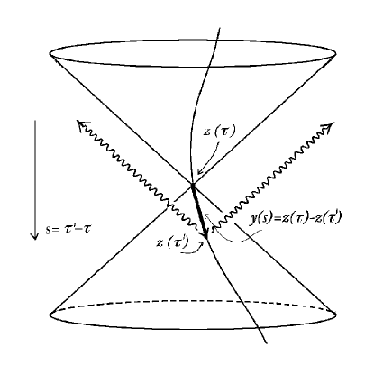
We may now transform the integral equation (87) to a local differential equation by expanding the functions around In Figure 1, we show a semiclassical trajectory with respect to the lightcone at Taking as fixed, we change integration variables using Next, we need the expansions
| (89) | ||||
| (90) | ||||
| (91) | ||||
| (92) | ||||
| (93) |
We set for convenience since we are concerned with the semiclassical limit. Also, we use and to simplify as necessary. We denote both by and by Using
| (94) | ||||
| (95) |
allows us to write the gradient operator as
| (96) | ||||
| (97) |
We also define
| (98) |
to be the total elapsed proper-time for the particle since the initial time . Recall that is defined by where is the initial time at which the state is defined.
These definitions and relations let us write the RHS of (87) as
| (99) | |||
| (100) | |||
| (101) |
where
| (102) | ||||
| (103) | ||||
| (104) | ||||
| (105) |
The functions depend on higher-derivatives of the particle coordinates up through order We next define the time-dependent parameters
| (106) |
and
| (107) | ||||
| (108) |
where is the Gamma function, is the incomplete Gamma function, and The constant depends on the details of the high-energy cutoff, but is of order one for reasonable cutoffs.
The coefficients are bounded for all including the limit In fact,
| (109) |
taking either limit. Therefore, we are free to exchange the sum over and the integration over to find a convergent series expansion of (87). The resulting local equations of motion are
| (110) | |||
| (111) |
From (102) we see that the terms give time-dependent mass renormalization; we accordingly define the renormalized mass as
| (112) | ||||
| (113) |
Similarly, the term is the usual third derivative radiation reaction force from the ALD equation. Thus, the equations of motion may be written as
| (114) |
where
| (115) |
These semiclassical equations of motion are almost of the Abraham-Lorentz-Dirac form, except for the time-dependent renormalization of the effective mass, the time-dependent (non-Markovian) radiation reaction force, and the presence of higher than third-time-derivative terms. The mass renormalization is to be expected, indeed it occurs in the classical derivation as well. What an initial-value formulation reveals is that renormalization effects are time-dependent owing to the nonequilibrium dynamics of particle-field interactions. The reason why renormalization is viewed as a time-independent procedure is because one usually only deals with equilibrium conditions or asymptotic in-out scattering problems.
IV Renormalization, causality, and runaways
A Time-dependent mass renormalization
The time-dependence of the effective mass (and particularly the radiation reaction coefficients ) play crucial roles in the semiclassical behavior. The initial particle at time is assumed, by our choice of initial state, to be fully uncorrelated with the field. This means the particle’s initial mass is just its bare mass Interactions between the particle and field then re-dress the particle state, one of the consequences being that the particle acquires a cloud of virtual field excitations (quanta) that change its effective mass. For a particle coupled to a scalar field there are two types of mass renormalization effects, one coming from the interaction, and the other coming from the interaction. We commented in Section II.C that the latter interaction is essentially a scalar field version of the electromagnetic coupling, if one defines the scalar field analog of the field strength tensor
We find that this interaction contributes a mass shift at late times of
| (116) |
In Paper III it is shown that is just one half the mass shift that is found when the particle moves in the electromagnetic field. This is consistent with the interpretation of the electromagnetic field as equivalent to two scalar fields (one for each polarization); therefore one expects, and finds, twice the mass renormalization in the electromagnetic case. (For the same reason we see below that the radiation reaction force, and stochastic noise, are each also reduced by half compared to the electromagnetic case.)
But the scalar field, unlike the electromagnetic field, also has a interaction that gives a mass shift The combined mass shift is then negative. At late-times, the renormalized mass is
| (117) | ||||
| (118) | ||||
| (119) | ||||
| (120) |
For a fixed if the cutoff satisfies the renormalized mass becomes negative and the equations of motion become unstable. It is well-known that environments with overly large cutoffs can qualitative change the system dynamics. In the following we will assume that the bare mass and cutoff are such that which in turn implies that and gives a bound on the cutoff:
(which is of the order of the inverse classical electron radius). We emphasize that for the scalar field case the field interaction reduces the effective particle mass, whereas in the electromagnetic (vector) field case the field interaction increases the effective particle mass (see paper III [2]). If we followed the FOL [17, 27, 28, 29] suggestion of picking a cutoff we would then conclude that as a consequence of the opposite sign in the mass renormalization effect. This is a kind of “critical” case balanced between stable and unstable particle motion, and while there may be special instances where such behavior is of interest, it does not seem to represent the generic behavior of typical (massive) particles interacting with scalar field degrees of freedom. We will defer further comparison with EM quantum Langevin equations to Paper III [2] where the mass renormalization has the more familiar sign.
We should further elaborate, however, on the role of causality in the equations of motion. In the preceding paragraph we see that for the long-term motion to be stable (i.e. positive effective particle mass) there is an upper bound on the field cutoff. This is well-known, as detailed in [17, 27, 28, 29], for example. There, the QLE is assumed to be of the form
| (121) |
where the time integration runs from to Causality is related to the analyticity of (the Fourier transform of ) in the upper half plane of the complex variable The traditional QLE of the type (121) with the lower integration limit set as effectively makes the assumption that the particle has been in contact with its environment far longer than the bath memory time. In our analysis the lower limit in (87) is not , because it is the (nonequilibrium) dynamics at early times immediately after the initial particle/field state is prepared where we have something new to say about how causality is preserved, and runaways are avoided.
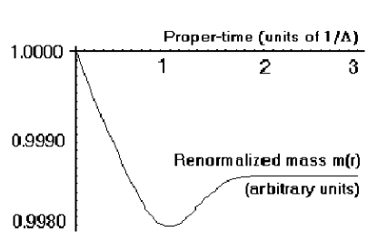
The proper-time dependence of the mass renormalization is shown in Figure 2. The horizontal axis marks the proper time in units of the cutoff timescale The vertical scale is arbitrary, depending on the particle mass. Notice one unusual feature: the mass shift is not monotonic with time, but instead first overshoots its final asymptotic value. This occurs because there are two competing mass renormalizing interactions that have slightly different timescales. The time-dependent mass-shift is a rapid effect, the final dressed mass is reached within a few
B Nonequilibrium radiation reaction
The constants determine how quickly the particle is able to rebuild its own self-field, which in turn controls the backreaction on the particle motion, ensuring that it is causal. We have found, as is typical of effective field theories, that the equations of motion involve higher derivative terms (i.e. for ) beyond the usual ALD form. In fact, all higher derivative terms are in principle present so long as they respect the fundamental symmetries (e.g., Lorentz and reparametrization invariance) of our particle-field model. The timescales and relative contributions of these higher-derivative forces are determined by the coefficients For a fixed cutoff the late-time behavior of the scale as
| (122) |
Therefore, the term has the late-time limit
| (123) |
which is independent of In the terminology of effective field theory, this makes the term renormalizable and implies that it corresponds to a ‘marginal’ coupling or interaction. In the same terminology the mass renormalization, scaling as corresponds to a relevant (renormalizable) coupling. In this vein, the higher-derivative corrections proportional to , suppressed by powers of the high-energy scale correspond to so-called irrelevant couplings.
If we had written the most general action for the particle-field system consistent with Lorentz and reparametrization invariance, we should have included from the beginning higher-derivative interactions. The effective field theory methodology when carried out fully shows that these high-derivative interactions are in fact irrelevant at low-energies. Therefore, the ordinary ALD form for radiation reaction (e.g., the term) results not as a consequence of the details of the ‘true’ high-energy theory, but because any Lorentz and reparametrization invariant effective theory behaves like a renormalizable particle-field theory that has the ALD equation as the low-energy limit. With this we come to the important conclusion that for a wide class of theories with the appropriate symmetries the low-energy limit of radiation reaction for (center of mass) particle motion is given by the ALD result. For theories with additional structure (such as spin), there will of course be additional radiation reaction terms important at the energy scale associated with the additional structure.
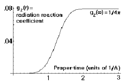
In Figure 3 we show the proper-time dependence of , with the same horizontal timescale as in Figure 2. It is evident that the radiation reaction force approaches the ALD form quickly, essentially on the cutoff time. While the radiation reaction force is non-Markovian, the memory time of the field-environment is very short. The non-Markovian evolution is characterized by the dependence of the coefficients and on the initial time but become effectively independent of after This is an example of the well-known behavior for quantum Brownian motion models found in [44]. The effectively transient nature of the short-time behavior helps justify our use of an initially uncorrelated (factorizable) particle and field state.
Also notice the role played by the particle’s elapsed proper-time, For particles with small average velocities††††††The small velocity approximation is relative to a choice of reference frame. In paper I (see Appenix A) we discuss how the choice of initially factorized state at some time picks out a special frame. the particle’s proper-time is roughly the background Minkowski time coordinate In this case, the time-dependences of the renormalization effects are approximately the same as one would find in the non-relativistic situation, since . For rapidly moving particles time-dilation can significantly lengthen the observed timescales with respect to the background Minkowski time. This indicates that highly relativistic particles will take longer (with respect to background time to equilibrate with the quantum field/environment than do more slowly moving particles. Finally, we note that the radiation reaction force is exactly half that found for the electromagnetic field.
C Causality and early-time behavior
We have shown that at low-energies and late-times the ALD radiation reaction force is generic (neglecting other particle structure, such as spin, which gives rise to additional low-energy corrections). But the classical ALD equation is plagued with pathologies like acausal and runaway solutions. The equations of motion in the form (87) are clearly unique and causal, they require only ordinary initial data, and do not have runaway solutions. However, it is instructive to see how the equations of motions in the form (114,115), involving higher derivatives, preserve the causal nature of the solutions with radiation reaction. To address these questions we now examine the early-time behavior of the equations of motion.
The presence of higher derivatives in (115) is an inevitable consequence of converting from a set of nonlocal integral equation (87) to a set of local differential equations (114,115). As differential equations, (114,115) may seem to be unphysical at first-sight because of the apparent need to specify initial data for But the coupling constants satisfy the crucial property that
| (124) |
for all We see this graphically for in Figure 3, and analytically for all in (107). Consequently, the particle self-force at identically vanishes (to all orders), and only smoothly rebuilds as the particle’s self-field is reconstituted. Therefore, the initial data at is fully (and uniquely) determined by
| (125) |
which only requires the ordinary Newtonian initial data. The initial values for the higher derivative terms (e.g. ) in (115) are determined iteratively from
| (126) |
Given the (Newtonian) initial data, the equations of motion are determined uniquely for all later times, to any order in In the classical ALD equations, one finds runaways even in the case of vanishing external potential, In our case, because for all if for all With these initial conditions (and the equations of motion (114,115) are
| (127) |
with unique solutions
| (128) |
Runaways do not arise.
As in the classical derivation of the Abraham-Lorentz-Dirac equation, these semiclassical equations of motion are equivalent to a second order differential-integral equation. In the classical case the integral equations are “derived” from the third-order ALD equation. If one chooses boundary conditions for the integral equation that eliminate runaways, one inevitably introduces pre-accelerated solutions. In our case, we derive the higher-derivative equations of motion (114,115) from the explicitly casual non-local integral equation (87). In doing this we avoid introducing unphysical solutions at short times as a consequence of the initially vanishing time-dependent parameters This turns out to be true for any good regularization of the field’s Green functions.
V The stochastic regime and the ALD-Langevin equation
A Single particle stochastic limit
The nonlinear Langevin equation in (65) shows a complex relationship between noise and radiation reaction. A nonlinear Langevin equation similar to these have been found in stochastic gravity by Hu and Matacz [35] describing the stochastic behavior of the gravitational field in response to quantum fluctuations of the stress-energy tensor. We now apply the results in Paper I (see Section IV [1]) giving the linearized Langevin equation for fluctuations around the mean trajectory. In the Langevin equation (65) we define where is the semiclassical solution from the previous section, and we work to first order in the fluctuation variable The free kinetic term is given by
| (129) | |||
| (130) | |||
| (131) |
where we have included the time-dependent mass renormalization effect in the kinetic term. The external potential term is
| (132) |
hence, the second derivative of acts as a force linearly coupled to The dissipative term for involves the (functional) derivative of the first cumulant (see Eq. (110)) with the mass renormalization term removed, as it has already been included in the kinetic term (131) above. We therefore need the (functional) derivative with respect to of the radiation reaction term
| (133) |
To we have
| (134) |
We note that is a function of the derivatives with therefore we have
| (135) | ||||
| (136) |
where are partial derivatives with respect to the derivative of The sum over terminates at since only contains derivatives up through order Hence, the Langevin equations for the fluctuations (around are
| (137) | |||
| (138) |
These are solved with found from (114). The noise is given by
| (139) |
where the lowest order noise is evaluated using the semiclassical solution
The correlator (see Eq. 145) is then found using the field correlator along the mean-trajectory:
| (140) |
Equation (139) shows that the noise experienced by the particle depends not just on the stochastic properties of the quantum field, but on the mean-solution For instance, the term in (139) gives noise that is proportional to the average particle acceleration. The second term in (139) depends on the antisymmetrized combination It follows immediately from that
From (145), we see that the noise correlator is
| (141) | |||
| (142) | |||
| (143) | |||
| (144) | |||
| (145) | |||
| (146) |
We have defined and The noise (when the field is initially in its vacuum state) is highly nonlocal, reflecting the highly correlated nature of the quantum vacuum. Only in the high temperature limit does the noise become approximately local. Notice that the noise correlator inherits an implicit dependence on the initial conditions at through the time-dependent equations of motion for But when the equations of motion become effectively independent of the initial time. The noise given by (145) is not stationary except for special cases of the solution
Since the terms represent high-energy corrections suppressed by powers of the low-energy Langevin equations are well approximated by keeping only the term. The linear dissipation () term becomes, using
| (147) | |||
| (148) | |||
| (149) | |||
| (150) |
where
| (151) | ||||
| (152) |
and This lowest order expression for dissipation in the equations of motion for involves time derivatives of through third order. However, just as was the case for the semiclassical equations of motion, the vanishing of for implies that the initial data for the equations of motion are just the ordinary kind involving no higher than first order derivatives. The lowest-order late-time ( single particle Langevin equations are thus
| (153) | ||||
| (154) |
B Multiparticle stochastic limit and stochastic Ward identities
It is a straightforward generalization to construct multiparticle Langevin equations. The two additional features are particle-particle interactions, and particle-particle correlations. The semiclassical limit is modified by the addition of the terms
| (155) |
The use of the regulated is essential for consistency between the radiation that is emitted during the regime of time-dependent renormalization and radiation-reaction; it ensures agreement between the work done by radiation-reaction and the radiant energy. A field cutoff implies that the radiation wave front emitted at is smoothed on a time scale .
We note one significant difference between the single particle and multiparticle theories. For a single particle, the dissipation is local (when the field is massless), and the semiclassical limit (obtaining when is essentially Markovian. The multiparticle theory is non-Markovian even in the semiclassical limit because of multiparticle interactions. Particle A may indirectly depend on its own past state of motion through the emission of radiation which interacts with another particle B, which in turn, emits radiation that re-influences particle A at some point in the future. The nonlocal field degrees of freedom stores information (in the form of radiation) about the particle’s past. Only for a single timelike particle in flat space without boundaries is this information permanently lost insofar as the particle’s future motion is concerned. These well-known facts make the multiparticle behavior extremely complicated.
We may evaluate the integral in (155) using the identity
| (156) |
where is the time when particle crosses particle past lightcone. (The regulated Green’s function would spread this out over approximately a time Defining , we use
| (157) | |||
| (158) | |||
| (159) | |||
| (160) |
The particle-particle interaction terms are then given by
| (161) | |||
| (162) | |||
| (163) |
where, as before, the acts only on the and not the Eq. (161) are just the scalar analog of the Liénard-Wiechert forces. They include both the near-field and far-field effects.
The long range particle-particle terms in the Langevin equations are found using (73), so we have the additional Langevin term for the th particle, found from
| (164) | |||
| (165) |
Equation (164) contains no third (or higher) derivative terms. The multiparticle noise correlator is
| (166) |
In general, particle-particle correlations between spacelike separated points will not vanish as a consequence of the nonlocal correlations implicitly encoded by For instance, when there are two oppositely charged particles which never enter each other’s causal future, there will be no particle-particle interactions mediated by however, the particles will still be correlated through the field vacuum via . This shows that it will not be possible to find a generalized multiparticle fluctuation-dissipation relation under all circumstances [39].
We now briefly consider general properties of the stochastic equations of motion. Notice that the noise satisfies the identity
| (167) |
which follows as a consequence of , for each particle number separately. This is an essential property since the particle fluctuations are real, not virtual. We may use (167) to prove what might be called (by analogy with QED) stochastic Ward-Takahashi identities [45]. The n-point correlation functions for the particle-noise are
| (168) | |||
| (169) | |||
| (170) |
with each acting on the corresponding These correlation functions may both involve different times along the worldline of one particle (i.e. self-particle noise), and correlations between different particles. From (168) and (167), follow “Ward” identities:
| (171) |
The contraction of on-shell momenta () with the stochastic correlation functions always vanishes. These identities are fundamental to the consistency of the relativistic Langevin equations.
VI Example: Free particles in the scalar field vacuum
As a concrete example, we find the Langevin equations for and the scalar field initially in the vacuum state. Using the stochastic equations of motion we can address the question of whether a free particle will experience Brownian motion induced by the vacuum fluctuations of the scalar field. When , we immediately see that for the semiclassical equations, constant; the radiation-reaction force identically vanishes (for all orders of ). The fact that uniquely fixes the constant as zero due to the initial data boundary conditions for the higher derivative terms (126); and hence, there are no runaway solutions characterized by a non-zero constant. We may write and where is a constant spacetime velocity vector which satisfies the (mass-shell) constraint A particle moving in accordance with the semiclassical solution neither radiates nor experiences radiation-reaction‡‡‡‡‡‡In constast, the mean-solution for a free particle in a quantum scalar field found in [46] does not possess the Galilean invariance of our results, and its motion is furthermore damped proportionally to its velocity.. Using we immediately find from (65) and (137) (using ) the (linear-order) Langevin equation
| (172) |
The noise correlator is found from (145) to be
| (173) | |||
| (174) | |||
| (175) | |||
| (176) | |||
| (177) |
where we have substituted the vacuum Hadamard function for the field-noise correlator The antisymmetric combination vanishes, and hence,
| (178) |
The origin of this at first surprising result is not hard to find. First, the “” dependant terms vanish since the average acceleration is zero, but why should the other terms in the correlator vanish? From (177), we see that the second term in the particle-noise correlator involves But the gradient of the vacuum Hadamard kernel (which is a function of ) satisfies and is therefore always in the direction of the spacetime vector connecting and However, for the inertial particle, , and thus the antisymmetrized term, always vanishes. It therefore follows that a scalar field with the coupling that we have assumed does not induce stochastic fluctuations in a free particles trajectory. This result is actually somewhat a special case for scalar fields, because in Paper III [2] we show that the electromagnetic field does induce stochastic fluctuations in a free particle. In the case of the electromagnetic field there is more freedom in (e.g., is a vector field; is the gradient of a scalar field) and so one does not find the cancellation that occurs above. For the case of a scalar field, there are noise-fluctuations when the field is not in the vacuum state (e.g. a thermal quantum field), and/or when the particle is subject to external forces that make its average acceleration non-zero (e.g. an accelerated particle).
We therefore find that the free particle fluctuations (in this special case) do not obey a Langevin equation. The equations of motion for are
| (179) |
Eq. (172) has the unique solution
| (180) |
after recalling that That is, the same initial time behavior that gives unique (runaway-free) solutions for (the semiclassical solution) apply to (the stochastic fluctuations).
Let us comment on the difference of our result from that of [46]. First, the dissipation term in our equations of motion is relativistically invariant for motion in the vacuum, and vanishes for inertial motion. The equations of motion in [46] are not; the authors concluded that a particle moving through the scalar vacuum will experience a dissipation force proportional to its velocity in direct contradiction with experience. This result comes from an incorrect treatment of the retarded Green’s function in 1+1 spacetime dimensions- which is quite different in behavior than the Green’s function in 3+1 dimensions. We avoid this problem by working in the more physical three spatial dimensions. We furthermore find that a free particle in the scalar vacuum does not experience noise (at least at the one-loop order of our derivation- see Paper I). This result is somewhat special owing to the particular symmetries of the scalar theory. In Paper III, we find that charged particles experience noise in the electromagnetic field vacuum. We have not addressed in depth the degree of decoherence of the particle motion, and how well the Langevin equation approximates the quantum expectation values for the particle motion is still an open question that will depend on the particular parameters (e.g., mass, charge, state of the field) of the model.
Our result also differs from that of Ford and O’Connell, who propose that the field-cutoff take a special value with the consequence that a free electron experiences fluctuations without dissipation [28]. We have already argued why this assumption is unnecessary as a consequence of recognizing QED as an effective theory. We have also emphasized the distinction between radiation reaction and dissipation. Hence, we find that a free (or for that matter a uniformly accelerated) particle has vanishing average radiation reaction, but when there exists a fluctuating force inducing deviations from the free (or uniformly accelerated) trajectory, there is then a balancing dissipation backreaction force. What is a little unusual about the scalar-field-free-particle case is that the “overly simple” monopole coupling between the scalar field and particle does not lead to quantum fluctuation induced noise when the expectation value of the particles acceleration vanishes (i.e. for a free particle). In paper III [2], treating the electromagnetic (vector) field, there is quantum field induced noise and dissipation in the particle trajectory, for both free and accelerated motion.
VII Discussion
We now summarize the main results of this paper, what follows from here, and point out areas for potential applications of theoretical and practical values.
Perhaps the most significant difference between this and earlier work in terms of approach is the use of a particle-centric and initial value (causal) formulation of relativistic quantum field theory, in terms of world-line quantization and influence functional formalisms, with focus on the coarse-grained and stochastic effective actions and their derived stochastic equations of motion. This is a general approach whose range of applicability extends from the full quantum to the classical regime, and should not be viewed as an approximation scheme valid only for the semiclassical. There exists a great variety of physical problems where a particle-centric formulation is more adept than a field-centric formulation. The initial value formulation with full backreaction ensures the self-consistency and causal behavior of the equations of motion for the semiclassical limit of particles in QED whose solutions are pathology free– the ALD-Langevin equations.
For further development, in Paper III [2] we shall extend these results to spinless particles moving in the quantum electromagnetic field, where we need to deal with the issues of gauge invariance. We find that the electromagnetic field is a richer source of noise than the simpler scalar field treated here. The ALD-Langevin equations for charged particle motion in the quantum electromagnetic field derived in Paper III is of particular importance for quantum beam dynamics and heavy-ion physics. Applying the ALD-Langevin equations to a charged particle moving in a constant background electric field (with the quantum field in the vacuum state), we show that its motion experiences stochastic fluctuations that are identical to those experienced by a free particle (i.e., where there is no background electric or magnetic field) moving in a thermal quantum field. This is an example of the Unruh effect [47]. The same effect exists for the scalar field example treated in this work, but we leave the essentially identical derivation for the more physically relevant case of QED presented in [2].
In a second series of papers [34], we use the same conceptual framework and methodology but go beyond the semiclassical and stochastic regimes to incorporate the full range of quantum phenomena, addressing questions such as the role of dissipation and correlation in charged particle pair-creation, and other quantum relativistic processes.
In conclusion, our approach is appropriate for any situation where particle motion (as opposed to field properties, say) is the center of attention. Our methods can be applied to relativistic charged particle motion not only in charged particle beams as in accelerators, and free-electron-lasers as in ion-optics, but also in strong fields such as particles moving in matter (crystals) or in plasma media as in astrophysical contexts [48].
Self-consistent treatment of backreaction from quantum field activities on a charged particle is an essential yet often neglected factor in many problems dealing with charged particle motion. First principles microscopic approach by means of covariant quantum field theory leading to microscopic stochastic equation is an effective remedy to this deficiency.
Theoretically, by interpreting a particle’s spacetime properties (e.g. its location in time and space) as effectively microscopic ‘clocks and position markers’ (e.g. events) we see that a quantum-covariant description of particle ‘worldline’ motion is not just particle dynamics, it is the quantum dynamics of spacetime events. For example, the “time” of the particle is treated as quantum variable on equal footing with position, and hence question like localization apply not just to localization in space, but localization in time. It would be natural to apply this approach to subjects like ‘time of flight’, that have become popular, and questions regarding decoherence of time (variables), together with space variables (e.g. the emergence of (local) time for particles).
Acknowledgments
This work is supported by NSF grant PHY98-00967 and DOE grant DEFG0296ER40949.
REFERENCES
- [1] P.R. Johnson and B.L. Hu, Stochastic Theory of Relativistic Particles Moving in a Quantum Field: I. Influence Functional and Langevin Equation, quant-ph/0012137 (2000).
- [2] P.R. Johnson and B.L. Hu, Stochastic Theory of Relativistic Particles Moving in a Quantum Field: III. Electromagnetic Abraham-Lorentz-Dirac-Langevin Equation and Unruh Effect, Preprint (2000); a summary of this series may be found in: P.R. Johnson and B.L. Hu, Worldline Influence Functional: Abraham-Lorentz-Dirac Equation from QED, to appear in Proceedings of the Second Conference on Quantum Aspects of Beam Physics (2000), edited by Pisin Chen (World Scientific, Singapore, 2001), quanta-ph/0012135.
- [3] E. Calzetta and B.L. Hu, in Directions in General Relativity, Vol. II: Brill Festschrift, edited by B.L. Hu and T.A. Jacobson (Cambridge University Press, Cambridge, 1993).
- [4] E. Calzetta and B.L. Hu, in Heat Kernel Techniques and Quantum Gravity, Vol. 4 of Discourses in Mathematics and Its Applications, Winnipeg, 1994, edited by S. A. Fulling (Texas AM University Press, College Station, TX, 1995), [Report No. hep-th/9501040].
- [5] C. Anastopoulos, Phys. Rev. D 54, 1600, (1996).
- [6] E. Calzetta and B.L. Hu, Phys. Rev. D 025012 (2000).
- [7] G.N. Plass, Rev. Mod. Phys. 33, 37 (1961); F. Rohrlich, Classical Charged Particles (Addison-Wesley, Reading, 1965).
- [8] P.W. Milonni, The Quantum Vacuum (Academic Press, Inc., San Diego, 1994).
- [9] M. Abraham and R. Becker, Electricity and Magnetism, Blackie, London, (1937); H.A. Lorentz, The Theory of Electrons (Dover Books, New York, 1952), pp. 49,253; P.A.M. Dirac, Proc. R. Soc. London A 167, 148 (1938).
- [10] P. Pearle, in Electromagnetism: Paths to Research, edited by D. Teplitz (Plenum Press, New York, 1982).
- [11] J. Wheeler and R. Feynman, Rev. Mod. Phys. 17, 157 (1945).
- [12] T. Fulton and F. Rohrlich, Ann. Phys. 9, 499 (1960).
- [13] F. Rohrlich, Am. J. Phys. 28, 639 (1969).
- [14] N.V. Kampen, Dan. Mat. Fys. Medd. 26, (1951); E. Moniz and D. Sharp, Phys. Rev. D 10, 1133 (1974); H. Levine, E. Moniz, and D. Sharp, Am. J. Phys. 45, 75 (1977).
- [15] H. Mori, Prog. Theor. Phys. 33, 423 (1965); G. W. Ford, M. Kac, and P. Masur, J. Math. Phys. 6, 504 (1965); H. Haken, Rev. Mod. Phys. 80, 67 (1975); H. Dekker, Phys. Rep. 80, 1 (1981).
- [16] A.O. Caldeira and A.J. Leggett, Ann. Phys. (N.Y.) 149, 374 (1983), and 153, 445(E) (1984).
- [17] G. W. Ford, J. T. Lewis, and R. F. O’Connell, Phys. Rev. Lett. 55, 2273 (1985); G. W. Ford, J. T. Lewis, and R. F. O’Connell, Phys. Rev. A 37, 4419 (1988).
- [18] M. Gell-Mann and J.B. Hartle, Phys. Rev. D 47, 3345 (1993); F. Dowker and A. Kent, Phys. Rev. Lett. 75, 3038 (1995); F. Dowker and A. Kent, J. Stat. Phys. 82, 1575 (1996).
- [19] E. Moniz and D. Sharp, Phys. Rev. D 15, 2850 (1977).
- [20] C. Cohen-Tannoudji, Atom-Photon Interactions (Wiley, New York, 1992).
- [21] P.W. Milonni, Phys. Lett. 82A, 225 (1981).
- [22] K. Wilson, Reviews of Modern Physics 55, 583 (1983); S. Weinberg, The Quantum Theory of Fields: Volume I: Foundations (Cambridge University Press, Cambridge, 1995); S. Weinberg, The Quantum Theory of Fields: Volume II: Modern Applications (Cambridge University Press, Cambridge, 1996).
- [23] A. J. Leggett et al., Rev. Mod. Phys. 59, 1 (1987); A. O. Caldeira and A. J. Leggett, Physica A 121, 587 (1983); V. Hakim and V. Ambegaokar, Phys. Rev. A 32, 423 (1985); F. Haake and R. Reibold, Phys. Rev. A 32, 2462 (1985), V. Hakim and V. Ambegaokar, Phys. Rev. A 32, 423 (1985), H. Grabert, P. Schramm, and G.-L. Ingold, Phys. Rev. Lett. 58, 1285 (1987).A. O. Caldeira and A. J. Leggett, Physica 121A, 587 (1988); B. L. Hu, J. P. Paz, and Y. Zhang, Phys. Rev. D 45, 2843 (1992); B.L. Hu, J.P. Paz, and Y. Zhang, Phys. Rev. D 47 1576 (1993).
- [24] W. H. Zurek, Phys. Rev. D 24, 1516 (1981); E. Joos and H. D. Zeh, Z. Phys. B 59, 223 (1985); W. G. Unruh and W. H. Zurek, Phys. Rev. D 40, 1071 (1989); A. O. Caldeira and A. J. Leggett, Phys. Rev. A 31, 1059 (1985).
- [25] P. Barone and A.O. Caldeira, Phys. Rev. A 43, 57 (1991).
- [26] L. D. Romero and J. P. Paz, [preprint: quant-ph/9612036] (1996).
- [27] G. W. Ford and R. F. O’Connell, Phys. Lett. A 157, 217 (1991).
- [28] G. W. Ford and R. F. O’Connell, Phys. Rev. A 57, 3112 (1998).
- [29] G. W. Ford and R. F. O’Connell, Phys. Lett. A 174, 182 (1993).
- [30] V. Krivitskii and V. Tsytovich, Sov. Phys. Usp. 34, 250 (1991).
- [31] F.E. Low, Annals Phys 266, 274 (1998).
- [32] L. Diósi, Found. Phys. 20, 63(1990).
- [33] L. H. Ford, Phys. Rev. D 47, 5571 (1993); L. H. Ford, Phys. Rev. A 56, 1812 (1997).
- [34] P.R. Johnson and B.L. Hu, Worldline Influence Functional, preprint (2000).
- [35] B.L. Hu and A. Matacz, Phys. Rev. D 51, 1577 (1995).
- [36] B.L. Hu, Int. J. Theor. Phys. 38, 2987 (1999).
- [37] R. Feynman and F. Vernon, Ann. Phys. 24, 118 (1963).
- [38] H. Callen and T. Welton, Phys. Rev. 83, 34 (1951).
- [39] A. Raval, B.L. Hu, and J. Anglin, Phys. Rev. D 53, 7003 (1996).
- [40] R.D. Jordan, Phys. Rev. D 33, 444 (1986).
- [41] E. Calzetta and B.L. Hu, Phys. Rev. D 35, 495 (1987).
- [42] T. Brun and J. J. Halliwell, Phys. Rev. D54, 2899, (1996); J. J. Halliwell, Phys. Rev. D58, 105015, (1998); J. J. Halliwell, Phys. Rev. Lett. 83, 2481, (1999); T.A. Brun and J.B. Hartle, Phys. Rev. D60, 123503, (1999).
- [43] J.B. Hartle, R. Laflamme and D. Marolf, Phys. Rev. D51, 7007, (1995).
- [44] B.L. Hu, J.P. Paz, and Y. Zhang, Phys. Rev. D 45, 2843 (1992).
- [45] J. Ward, Phys. Rev. 78, 182 (1950); Y. Takahashi, Nuovo Cim. 6, 371 (1957).
- [46] G. Gour and L. Sriramkumar, Foundations of Physics 29, 1917 (1999).
- [47] W. G. Unruh, Phys. Rev. D 14, 870 (1976).
- [48] Quantum Aspects of Beam Physics, Advanced IFCA Beam Dynamics Workshop, edited by P. Chen (World Scientific, Singapore, 1998).