Quantum Fluctuations of Radiation Pressure

Abstract

Quantum fluctuations of electromagnetic radiation pressure are discussed. We use an approach based on the quantum stress tensor to calculate the fluctuations in velocity and position of a mirror subjected to electromagnetic radiation. Our approach reveals that radiation pressure fluctuations are due to a cross term between vacuum and state dependent terms in a stress tensor operator product. Thus observation of these fluctuations would entail experimental confirmation of this cross term. We first analyze the pressure fluctuations on a single, perfectly reflecting mirror, and then study the case of an interferometer. This involves a study of the effects of multiple bounces in one arm, as well as the correlations of the pressure fluctuations between arms of the interferometer. In all cases, our results are consistent with those previously obtained by Caves using different mehods.

I Introduction

Classically, a beam of light falling on a mirror exerts a force and the force can be written as the integral of the Maxwell stress tensor. When we treat this problem quantum mechanically, then the force undergoes fluctuations. This is a necessary consequence of the fact that physically realizable quantum states are not eigenstates of the stress tensor operator. These radiation pressure fluctuations play an important role in limiting the sensitivity of laser interferometer detectors of gravitational radiation, as was first analyzed by Caves [1, 2]. His approach is based on the photon number fluctuations in a coherent state, and we will refer to it as the photon number approach. The purpose of this paper is to examine radiation pressure fluctuations using the quantum stress tensor. This requires the correlation function of a pair of stress tensor operators, which will be discussed in Sect. II. There it is shown that the correlation function can be decomposed into three parts, a term which is fully normal-ordered, a state independent vacuum term, and a “cross term” which can be viewed as an interference term between the vacuum fluctuations and the matter content of the quantum state. It is this cross term which will be of greatest interest in this paper, as it is responsible for the radiation pressure fluctuations in a coherent state. These fluctuations will be discussed in Sect. III for the case of a laser beam impinging upon a single, perfectly reflecting mirror. The analysis will be done first using the photon number approach, and then using the stress tensor approach. In the latter case, we show how the calculations may be performed in coordinate space, where an integration over space and time is needed to remove a singularity in the cross term. We then show how to obtain the same result more simply using a othonormal basis of wavepacket modes. In Sect. III D, we examine the case of a single mode number eigenstate, and show that the radiation pressure fluctuations vanish. In the stress tensor approach, this arises from a cancellation between the cross term and the fully normal ordered term. In Sect. IV, we turn to the discussion of an interferometer. We first study the effects of mutiple bounces in a single arm, and reproduce the result [1, 2] that the effect of the radiation pressure fluctuations grows as the square of the number of bounces. We also show how our approach may be used to discuss the situation where the interferometer arms are Fabry-Perot cavities. Finally, we discuss the correlation between the fluctuations in the two interferometer arms, and show why they are in fact uncorrelated. Our results are summarized and discussed in Sect. V.

II Energy-momentum tensor fluctuations

It is well known that stress tensor operators can be renormalized by normal ordering:

$$:T_{\mu\nu}:=T_{\mu\nu}-\langle T_{\mu\nu}\rangle_{0}\,,$$ (1)

which is subtraction of the Minkowski vacuum expectation value. However, the quantity $\langle:T_{\mu\nu}(x)::T_{\rho\sigma}(x^{\prime}):\rangle$ is still divergent in the limit that $x^{\prime}\rightarrow x$. The divergent part of this quantity can be decomposed into a state-independent part and a state-dependent part. To do so, we may use the following identity, which follows from Wick’s theorem

$$:\phi_{1}\phi_{2}::\phi_{3}\phi_{4}: = :\phi_{1}\phi_{2}\phi_{3}\phi_{4}:$$ (5)

$$+:\phi_{1}\phi_{3}:\langle\phi_{2}\phi_{4}\rangle_{0}+:\phi_{1}\phi_{4}:\langle\phi_{2}\phi_{3}\rangle_{0}$$

$$+:\phi_{2}\phi_{3}:\langle\phi_{1}\phi_{4}\rangle_{0}+:\phi_{2}\phi_{4}:\langle\phi_{1}\phi_{3}\rangle_{0}$$

$$+\langle\phi_{1}\phi_{3}\rangle_{0}\langle\phi_{2}\phi_{4}\rangle_{0}+\langle\phi_{1}\phi_{4}\rangle_{0}\langle\phi_{2}\phi_{3}\rangle_{0}\,.$$

Here the $\phi_{i}$ are free bosonic fields and $\langle\,\rangle_{0}$ denotes the Minkowski vacuum expectation value. The first term is fully normal-ordered, the next four are cross terms and the final two are pure vacuum terms. The physics of these various terms was discussed in Ref. [3]. Here $\phi_{1}$ and $\phi_{2}$ are evaluated at point $x$, whereas $\phi_{3}$ and $\phi_{4}$ are evaluated at point $x^{\prime}$. In the coincidence limit, $x^{\prime}\rightarrow x$, the fully normal-ordered term is finite, but the cross term and vacuum terms diverge. The singularity of the cross term is of particular significance because, unlike the vacuum term, it is state-dependent. The fully normal-ordered term will not contribute to the fluctuations so long as the quantum state is a coherent state. The pure vacuum term will also not contribute so long as we restrict our attention to the differences between a given quantum state and the vacuum state.

If the quantum state is other than a coherent state, there are also state-dependent stress tensor fluctuations in the fully normal ordered term. These fluctuations were discussed in Refs. [4, 5, 6, 7], especially in a context where the stress tensor is the source of gravity. The normal ordered term is always finite and does not present a divergence problem, in contrast to the cross term. The latter term can only be made meaningful if one examines space or time integrated quantities and has a prescription for defining the resulting integrals. We may schematically express the expectation value of a product of stress tensor operators as

$$\langle:T_{\mu\nu}::T_{\rho\sigma}:\rangle=\langle:T_{\mu\nu}T_{\rho\sigma}:\rangle+\langle T_{\mu\nu}T_{\rho\sigma}\rangle_{cross}+\langle T_{\mu\nu}T_{\rho\sigma}\rangle_{0}\,,$$ (6)

where the three terms of the right hand side are, respectively, the fully normal ordered term, the cross term, and the vacuum term. For a single mode coherent state $|z\rangle$,

$$\langle z|:T_{\mu\nu}T_{\rho\sigma}:|z\rangle=\langle z|:T_{\mu\nu}:|z\rangle\langle z|:T_{\rho\sigma}:|z\rangle\,.$$ (7)

In such a state, the fluctuations of the stress tensor are described by quantities of the form

$$\langle\triangle T^{2}\rangle=\langle:T_{\mu\nu}:^{2}\rangle-\langle:T_{\mu\nu}:\rangle^{2}=\langle:T_{\mu\nu}:^{2}\rangle_{cross}+\langle:T_{\mu\nu}:^{2}\rangle_{0}\,.$$ (8)

If we are interested only in the changes in $\langle\triangle T^{2}\rangle$ when the quantum state is varied, then the pure vacuum term can be ignored, and only the cross term is important:

$$\langle\triangle T^{2}\rangle\rightarrow\langle:T_{\mu\nu}:^{2}\rangle_{cross}\,.$$ (9)

Note that we do not mean to suggest that there is no physical meaning to the pure vacuum term. It presumably describes fluctuations of the stress tensor components in the Minkowski vacuum state. More precisely, if one measures a spacetime averaged component, the result of the measurement should undergo fluctuations which vary as an inverse power of the size of the averaging region. However, in a non-vacuum state, the magnitude of the cross term will grow as the mean energy density in the state. Thus there will be a regime in which the effects of the cross term dominate those of the vacuum term.

We must resolve the issue of the state-dependent divergences in the cross term if it is to have any physical content. This issue was discussed by us in Ref. [3], where it was shown that although the stress tensor correlation function is singular in the coincidence limit, integrals of this function over space and time can still be well-defined. The cross term in the stress tensor correlation function has the form

$$\langle T_{\mu\nu}(x)T_{\rho\sigma}(x^{\prime})\rangle_{cross}=\frac{F(x,x^{\prime})}{(x-x^{\prime})^{4}}\,,$$ (10)

where $F(x,x^{\prime})$ is a regular function of the spacetime points $x$ and $x^{\prime}$, and $(x-x^{\prime})^{2}$ is the squared geodesic distance between them. Integrals of the correlation function appear to be formally divergent, but nonetheless may be defined by an integration by parts procedure. Suppose for the sake of illustration that the integrations are over time only, and note that

$$\frac{1}{(t-t^{\prime})^{4}}=-\frac{1}{12}\,\frac{\partial^{2}}{\partial t^{2}}\frac{\partial^{2}}{\partial t^{\prime 2}}\ln(t-t^{\prime})^{2}\,.$$ (11)

If the function $F$ vanishes sufficiently rapidly at the endpoints of the integrations, we can write

$$\int dt\,dt^{\prime}\frac{F(t,t^{\prime})}{(t-t^{\prime})^{4}}=-\frac{1}{12}\,\int dt\,dt^{\prime}\ln(t-t^{\prime})^{2}\,\frac{\partial^{2}}{\partial t^{2}}\frac{\partial^{2}}{\partial t^{\prime 2}}\,F(t,t^{\prime})\,.$$ (12)

This procedure provides a way to define integrals with singular integrands, and has been discussed by various authors [8, 9]. As we will see below in Sect. III B and in the Appendix, the integrals of the cross term which describe radiation pressure fluctuations can be made finite by a similar procedure.

III Induced Momentum Fluctuations of a Single Mirror

It is well known from classical physics that a beam of light falling on a reflecting or absorbing surface exerts a pressure. This pressure may be computed by integration of the appropriate component of the Maxwell stress tensor over the surface. It may also be computed by counting photon momenta. Let us illustrate the latter method, which we will call the “photon number” approach. If an incident monochromatic beam of angular frequency $\omega$ and energy density $\rho$ strikes a surface, the mean number of photons striking per unit time per unit area is $\rho/\omega$. If the light is perfectly reflected, each photon imparts a momentum $2\omega$ to the surface, resulting in a radiation pressure of $2\rho$. As expected, both the stress tensor and the photon number approaches yield the same answer.

However, these calculation give only a mean value. The radiation pressure should undergo fluctuations about this mean. In the photon number viewpoint, these fluctuations arise from fluctuations in the rate of photons striking the surface. In the stress tensor viewpoint, the fluctuations arise because the quantum state of the radiation field is not an eigenstate of pressure. The main purpose of this section is to examine radiation pressure fluctuations in a single mode coherent state from both viewpoints, and to compare the results. In one subsection, Sect. III D, we will also examine the case of a single mode photon number eigenstate.

A The Photon Number Approach

In this approach, the radiation pressure fluctuates because of statistical fluctuations in the numbers of photons striking the surface. Suppose that a beam of light with angular frequency $\omega$ is described by a single mode coherent state, $|z\rangle$, an eigenstate of the annihilation operator, $a|z\rangle=z|z\rangle$. The mean number of photons which strike a mirror in time $\tau$ is

$$\langle n\rangle=\langle a^{\dagger}a\rangle=|z|^{2}\,.$$ (13)

If the mirror is perfectly reflecting, then the mean momentum transferred is the expectation value of the operator

$$p=2\omega n\,.$$ (14)

The dispersion of this momentum is given by

$$\langle\Delta p^{2}\rangle=\langle p^{2}\rangle-\langle p\rangle^{2}=4\omega^{2}(\langle n^{2}\rangle-\langle n\rangle^{2})\,.$$ (15)

In a coherent state,

$$\langle n^{2}\rangle-\langle n\rangle^{2}=\langle a^{\dagger}aa^{\dagger}a\rangle-\langle a^{\dagger}a\rangle^{2}=\langle(a^{\dagger})^{2}a^{2}\rangle+\langle a^{\dagger}a\rangle-\langle a^{\dagger}a\rangle^{2}=\langle a^{\dagger}a\rangle=\langle n\rangle\,.$$ (16)

Thus

$$\langle\Delta p^{2}\rangle=4\omega^{2}\langle n\rangle=4\omega\,A\rho\,\tau\,,$$ (17)

where $\rho$ is the mean energy density of the incident beam, and $A$ is its cross sectional area. If the mirror is a free body with mass $m$, the mean squared velocity fluctuation is

$$\langle\Delta v^{2}\rangle=4\frac{\omega A\rho}{m^{2}}\tau\,.$$ (18)

B The Stress Tensor Approach

An alternative approach to the problem of radiation pressure fluctuations is the method of stress tensor fluctuations. It is well known that one can calculate the force on a surface by integration of the relevant component of the stress tensor over that surface. It thus seems reasonable to expect that the fluctuations in this force can also be computed from the quantum stress tensor. There is, however, a problem which needs to be resolved in this approach. This is that products of stress tensor operators are not well defined at coincident points. Even the integrals of these products are formally divergent and need a regularization. A regularization scheme was used in our previous work [3] and will be adopted again in this paper. The main idea is to treat the measuring process as a switch-on-switch-off process and do an integrations by parts.

Consider a mirror of mass $m$ which is oriented perpendicularly to the $x$-direction. If the mirror is at rest at time $t=0$, then at time $t=\tau$ its velocity in the $x$-direction is given classically by

$$v=\frac{1}{m}\int_{0}^{\tau}dt\int_{A}da\,\,T_{xx}\,,$$ (19)

where $T_{ij}$ is the Maxwell stress tensor, and $\int_{A}da$ denotes an integration over the surface of the mirror. Here we assume that there is radiation present on one side of the mirror only. Otherwise, Eq. (19) would involve a difference in $T_{xx}$ across the mirror. When the radiation field is quantized, $T_{ij}$ is replaced by the normal ordered operator $:T_{ij}:$, and Eq. (19) becomes a Langevin equation. The dispersion in the mirror’s velocity becomes

$$\langle\triangle v^{2}\rangle=\frac{1}{m^{2}}\int_{0}^{\tau}dt\,\int_{0}^{\tau}dt^{\prime}\,\int_{A}da\,\int_{A}da^{\prime}\,[\langle:T_{xx}(x)::T_{xx}(x^{\prime}):\rangle-\langle:T_{xx}(x):\rangle\langle:T_{xx}(x^{\prime}):\rangle]$$ (20)

As discussed above, when the quantum state of the radiation field is a coherent state and we ignore the pure vacuum term, then the dispersion in $T_{xx}$ is given by the cross term alone, and

$$\langle\triangle v^{2}\rangle=\frac{1}{m^{2}}\int_{0}^{\tau}dt\int_{0}^{\tau}dt^{\prime}\int_{A}da\int_{A}da^{\prime}\langle T_{xx}(x)T_{xx}(x^{\prime})\rangle_{cross}\,.$$ (21)

The components of the energy-momentum tensor for the electromagnetic field are (Lorentz-Heaviside units are used here.)

$$T^{ij} = \delta^{ij}T^{00}-(E^{i}E^{j}+B^{i}B^{j})\,,$$ (22)

$$T^{0i} = \epsilon^{ijk}E^{j}B^{k}\,,$$ (23)

and

$$T^{00}=\frac{1}{2}(E^{2}+B^{2})\,.$$ (24)

Here $E^{i}$ and $B^{i}$ are Cartesian components of the electric and magnetic fields, respectively. In particular,

$$T_{xx}=\frac{1}{2}(E_{y}^{2}+E_{z}^{2}+B_{y}^{2}+B_{z}^{2})\,.$$ (25)

We now assume that a linearly polarized plane wave is normally incident and is perfectly reflected by the mirror. Take the polarization vector to be in the $y$-direction, so that $E_{z}=B_{y}=0$. At the location of the mirror, $E_{y}=0$, and only $B_{z}$ contributes to the stress tensor. Thus, when we apply Eq. (5) to find $\langle T_{xx}(x)T_{xx}(x^{\prime})\rangle_{cross}$, the only nonzero quadratic normal-ordered product will be $\langle:B_{z}(x)B_{z}(x^{\prime}):\rangle$. The result is

$$\langle T_{xx}(x)T_{xx}(x^{\prime})\rangle_{cross}=\langle:B_{z}(x)B_{z}(x^{\prime}):\rangle\langle B_{z}(x)B_{z}(x^{\prime})\rangle_{0}\,.$$ (26)

The $z$-component of the magnetic field operator may be expressed in terms of mode functions as

$$B_{z}(x)=\sum_{\omega}(a_{\omega}\,B_{\omega}+a_{\omega}^{\dagger}\,B_{\omega}^{*})\,,$$ (27)

where the mode function is

$$B_{\omega}=-2\,C\cos(\omega x)\,e^{-i\omega t}\,.$$ (28)

Here C is the coefficient for box normalization in a volume $V$

$$C=\sqrt{\frac{\omega}{2V}}\,.$$ (29)

The coherent state is an eigenstate of the annihilation operator

$$a_{\omega^{\prime}}|z\rangle=\delta_{\omega^{\prime}\omega}z|z\rangle\,,$$ (30)

where $z$ is a complex number

$$z=|z|e^{-i\phi}\,.$$ (31)

The expectation value of the normal ordered product of field operators is now

$$\langle z|:B_{z}(t_{1})B_{z}(t_{2}):|z\rangle=16C^{2}|z|^{2}\cos(\omega t_{1}+\phi)\cos(\omega t_{2}+\phi)\cos(\omega x_{1})\cos(\omega x_{2})$$ (32)

The vacuum magnetic field two-point function in the presence of a perfectly reflecting plane at $z=0$ is given by

$$\langle B_{z}(t_{1},{\textbf{x}}_{1})B_{z}(t_{2},{\textbf{x}}_{2})\rangle_{0}=\langle B_{z}(t_{1},{\textbf{x}}_{1})B_{z}(t_{2},{\textbf{x}}_{2})\rangle_{E0}+\langle B_{z}(t_{1},{\textbf{x}}_{1})B_{z}(t_{2},{\textbf{x}}_{2})\rangle_{I0}\,.$$ (33)

The first term is the two-point function for empty space,

$$\langle B_{z}(t_{1},{\textbf{x}}_{1})B_{z}(t_{2},{\textbf{x}}_{2})\rangle_{E0}=\frac{(t_{1}-t_{2})^{2}+|{\textbf{x}}_{1}-{\textbf{x}}_{2}|^{2}-2(z_{1}-z_{2})^{2}}{\pi^{2}[(t_{1}-t_{2})^{2}-|{\textbf{x}}_{1}-{\textbf{x}}_{2}|^{2}]^{3}}\,.$$ (34)

The second term is an image term

$$\langle B_{z}(t_{1},{\textbf{x}}_{1})B_{z}(t_{2},{\textbf{x}}_{2})\rangle_{I0}=\langle B_{z}(t_{1},{\textbf{x}}_{1})B_{z}(t_{2},{\textbf{x}}_{2})\rangle_{E0}\biggl{|}_{z_{2}\rightarrow-z_{2}}\,.$$ (35)

Both terms give equal contributions to the radiation pressure fluctuations on a mirror located at $z=0$.

We can now combine these results to write Eq. (21) as

$$\langle\triangle v^{2}\rangle=\frac{32C^{2}|z|^{2}}{\pi^{2}m^{2}}\int_{A}da_{1}\,\int da_{2}\,J$$ (36)

where

$$J=\int_{0}^{\tau}dt_{1}\int_{0}^{\tau}dt_{2}\frac{(t_{1}-t_{2})^{2}-a}{[(t_{1}-t_{2})^{2}-b^{2}]^{3}}\,\cos(\omega t_{1})\cos(\omega t_{2})\,,$$ (37)

with

$$a=(z_{1}-z_{2})^{2}-(y_{1}-y_{2})^{2}$$ (38)

and

$$b^{2}=(y_{1}-y_{2})^{2}+(z_{1}-z_{2})^{2}\,.$$ (39)

Here we have set $\phi=\arg(z)=0$, as it just shifts the origin of time, and taken the location of the mirror to be at $x=0$. The integral $J$ is evaluated in the Appendix in the limit of large $\tau$, with the result

$$J=\frac{2\pi\tau}{32b^{5}}\,\left\{\left[b^{2}(b^{2}+a)\omega^{2}+b^{2}-3a\right]\sin b\omega+\omega b(3a-b^{2})\cos b\omega\right\}\,.$$ (40)

The singularities in the integrand of Eq. (37) are third order poles, which are evaluated using an integration by parts.

We next need to perform the spatial integration over the area of the mirror which is illuminated by the laser beam. Assume that the illuminated region is a disk of radius $R$ and hence area $A=\pi R^{2}$, and that the incident flux is uniform over this disk. (This assumption is not essential, but simplifies the calculations.) If we take the origin for the $da_{1}$ integration to be at $y_{2}=z_{2}=0$, then

$$I \equiv \int_{A}da_{2}\int_{A}da_{1}\,[b^{2}(b^{2}+a)\omega^{2}+b^{2}-3a]\sin b\omega+\omega b(3a-b^{2})\cos b\omega]\,b^{-5}$$ (41)

$$= \int da_{2}\int_{0}^{R}r\,dr\int_{0}^{2\pi}d\theta\,\frac{1}{r^{5}}$$ (43)

$$\times\left[\omega r(r^{2}-3r^{2}\sin^{2}\theta)\cos(\omega r)+[3r^{2}\sin^{2}\theta+r^{4}\omega^{2}-r^{2}(1+r^{2}\sin^{2}\theta\omega^{2})]\sin(\omega r)\right]$$

$$= \pi\int da_{2}\int_{0}^{R}\frac{(1+\omega^{2}r^{2})\sin(\omega r)-\omega r\cos(\omega r)}{r^{2}}\,dr\,.$$ (44)

Further assume that $R\gg\omega^{-1}$. Then we can let $R\rightarrow\infty$ in the upper limit of the $r$ integration. The $da_{2}$ integration now simply contributes a faxtor of $A$, and we have

$$I \approx \pi A\int_{0}^{\infty}\frac{(1+\omega^{2}r^{2})\sin(\omega r)-\omega r\cos(\omega r)}{r^{2}}\,dr$$ (45)

$$= \pi\omega A\int_{0}^{\infty}\frac{(1+u^{2})\sin(u)-u\cos(u)}{u^{2}}\,du$$ (46)

$$= \pi\omega A\int_{0}^{\infty}\,du\,\left[\sin u-\frac{d}{du}\left(\frac{\sin u}{u}\right)\right]$$ (47)

$$= 2\pi\omega A\,.$$ (48)

In the last step, we used $\int_{0}^{\infty}\,du\,\sin u=\lim_{\alpha\rightarrow 0}\int_{0}^{\infty}\,du\,\sin u\,{\textrm{e}}^{-\alpha u}=1\,.$ Thus we have

$$\langle\triangle v^{2}\rangle=\frac{16\,C^{2}|z|^{2}\omega A\tau}{\pi m^{2}}\,.$$ (49)

The energy density in the incident wave can be written as

$$\rho=\frac{\omega|z|^{2}}{V}=2C^{2}|z|^{2}\,,$$ (50)

so we can express the velocity fluctuations as

$$\langle\triangle v^{2}\rangle=4\,\frac{A\omega\rho}{m^{2}}\,\tau\,.$$ (51)

Note that this result agrees with that from the photon counting approach, Eq. (18).

C The Wavepacket Approach

Here we wish to provide an alternative derivation of the momentum fluctuations of a single mirror using the stress tensor approach. Rather than performing all of the calculations in coordinate space, as was done in Sect. III B, we will use an approach based upon wavepacket modes. This approach will prove useful in discussing interferometer noise. Assume that the occupied mode is a wavepacket which is sharply peaked at frequency $\omega$. Using Eq. (21) and Eq. (26) for a coherent state, the momentum fluctuation becomes

$$\langle\triangle p^{2}\rangle = m^{2}\langle\triangle v^{2}\rangle$$ (52)

$$= \int dt\,da\,\int dt^{\prime}\,da^{\prime}\,\langle T_{xx}(x)T_{xx}(x^{\prime})\rangle_{cross}$$ (53)

$$= \int dt\,da\,\int dt^{\prime}\,da^{\prime}\langle:B_{z}(x)B_{z}(x^{\prime}):\rangle\langle B_{z}(x)B_{z}(x^{\prime})\rangle_{0}\,.$$ (54)

Let the magnetic field operator $B_{z}(x)$ be expanded in terms of a complete set of positive frequency wavepacket modes $\{u_{j}(x)\}$ :

$$B_{z}(x)=\sum_{j}[a_{j}\,u_{j}(x)+a_{j}^{\dagger}u_{j}^{*}(x)]\,.$$ (55)

For our purpose, we take these modes to be fairly sharply peaked in frequency and use the normalization condition

$$\int u_{j}^{*}u_{j^{\prime}}\,d^{3}x=\frac{1}{2}\omega_{j}\,\delta_{jj^{\prime}}\,,$$ (56)

where $\omega_{j}$ is the mean frequency of packet $j$. More generally, we should expand the vector potential ${\bf A}$ in terms of wavepackets $f_{j}$:

$\displaystyle{\bf A}=\sum_{j}(a_{j}\widehat{e_{j}}f_{j}+H.c.)\,,$where $\langle f_{j},f_{j^{\prime}}\rangle=\delta_{jj^{\prime}}$ and $\langle f_{j},f_{j^{\prime}}\rangle$ is the Klein-Gordon inner product. Then the modes $u_{j}$ are expressed as derivatives of the modes $f_{j}$. Consider a single mode coherent state $|z\rangle$ as the quantum state, and let the mode be a wavepacket $u_{0}$. Then with a suitable choice of the phase of this mode function, we can write

$$\langle:B_{z}(x)B_{z}(x^{\prime}):\rangle=|z|^{2}[u_{0}(x)+u_{0}^{*}(x)][u_{0}(x^{\prime})+u_{0}^{*}(x^{\prime})]\,.$$ (57)

Note that the integrals in $\langle\triangle p^{2}\rangle$ are of the form $\int dt\,da$ rather than $\int d^{3}x$ . If the integrand is a function of $t-x$ alone, or $t+x$ alone, these are equivalent:

$$\int_{-\infty}^{\infty}dt\,f(t-x)=\int_{-\infty}^{\infty}du\,f(u)=\int_{-\infty}^{\infty}du\,f(-u)=\int_{-\infty}^{\infty}dx\,f(t-x)$$ (58)

and

$$\int_{-\infty}^{\infty}dt\,f(t+x)=\int_{-\infty}^{\infty}dx\,f(t+x)\,,$$ (59)

where $u=t-x$. However, when the mirror is present, $u_{0}$ contains pieces moving in both directions:

$$u_{0}=u_{0I}+u_{0R\,,}$$ (60)

where $u_{0I}$ is the incident wavepacket and $u_{0R}$ is the reflected wavepacket. The key feature that we will use is that $u_{0}$ is orthogonal to $u_{j}$ ($j\neq 0$), but $u_{0I}$ and $u_{0R}$ are not orthogonal to each other. Inserting Eq. (55) and Eq. (57) into Eq. (54) yields

$$\langle\triangle p^{2}\rangle = |z|^{2}\int dt\,da\,\int dt^{\prime}\,da^{\prime}[u_{0}(x)+u_{0}^{*}(x)][u_{0}(x^{\prime})+u_{0}^{*}(x^{\prime})]$$ (62)

$$\times\frac{1}{2}\sum_{j}[u_{j}(x)u_{j}^{*}(x^{\prime})+u_{j}^{*}(x)u_{j}(x^{\prime})]$$

$$= |z|^{2}\sum_{j}Re\left[\int dt\,da\,\int dt^{\prime}\,da^{\prime}u_{0}(x)u_{0}^{*}(x^{\prime})u_{j}^{*}(x)u_{j}(x^{\prime})\right]$$ (63)

$$= |z|^{2}\sum_{j}Re\left[\int u_{0}(x)u_{j}^{*}(x)dt\,da^{\prime}\,\int u_{0}^{*}(x^{\prime})u_{j}(x^{\prime})dt^{\prime}\,da\right]$$ (64)

$$= |z|^{2}\left[\int u_{0}(x)u_{0}^{*}(x)dt\,da\right]^{2}\,.$$ (65)

Using Eq. (60), the integral in the last expression becomes

$$I = \int u_{0}(x)u_{0}^{*}(x)dt\,da$$ (66)

$$= \int dt\,da\,(u_{0I}+u_{0R})(u_{0I}^{*}+u_{0R}^{*})$$ (67)

$$= \int dt\,da\,(|u_{0I}|^{2}+|u_{0R}|^{2}+u_{0I}u_{0R}^{*}+u_{0I}^{*}u_{0R})\,.$$ (68)

Here the only difference between $u_{0I}$ and $u_{0R}$ is their direction of travel. If $u_{0I}=f(t-x)$, then $u_{0R}=f(t+x)$, and $u_{0I}=u_{0R}$ at the mirror, and

$$\int dt\,da\,u_{0I}u_{0R}^{*}=\int dt\,da\,u_{0I}^{*}u_{0R}=\int dt\,da\,|u_{0I}|^{2}=\int dt\,da\,|u_{0R}|^{2}\,.$$ (69)

Thus

$\displaystyle I=\int u_{0}(x)u_{0}^{*}(x)dt\,da=4\int dt\,da\,|u_{0I}|^{2}=4\int d^{3}x|u_{0I}|^{2}=2\omega\,,$and the momentum fluctuation becomes

$$\langle\triangle p^{2}\rangle=4\omega^{2}|z|^{2}=4\omega^{2}\langle n\rangle\,.$$ (70)

This is same as the result of the photon number counting approach, Eqs. (18), and of the integration by parts in Sect. III B, (51).

D A Number Eigenstate

Most of this paper deals with single mode coherent states. However, in this subsection, we wish to turn aside from the main line of development and discuss the case of a single mode number eigenstate. It is apparent in the photon number approach that there should not be any radiation pressure fluctuations in such a state. In the stress tensor approach, the situation is less clear, as both the fully normal-ordered term and the cross term are nonzero.

We assume that the quantum state $|n\rangle$ is a number eigenstate of a single mode. Expand the magnetic field operator in terms of complete set of mode functions using Eq. (27) to find the expectation value of the fully normal ordered term

$$\langle n|:T_{xx}(x)T_{xx}(x^{\prime}):|n\rangle$$ (71)

$$= \frac{1}{4}\langle n|:B_{z}^{2}(x)B_{z}^{2}(x^{\prime}):|n\rangle$$ (72)

$$= \frac{1}{4}n(n-1)[B_{\omega}^{*2}(x)B_{\omega}^{2}(x^{\prime})+B_{\omega}^{2}(x)B_{\omega}^{*2}(x^{\prime})+4|B_{\omega}(x)|^{2}|B_{\omega}(x^{\prime})|^{2}]\,.$$ (73)

Here $B_{\omega}$ is the mode function for the occupied mode, and is assumed to be given by Eqs. (28) and (29). A similar procedure leads to the result for the cross term

$$\langle n|:T_{xx}(x)::T_{xx}(x^{\prime}):|n\rangle_{cross}$$ (74)

$$= \langle n|:B_{z}(x)B_{z}(x^{\prime}):|n\rangle\langle B_{z}(x)B_{z}(x^{\prime})\rangle_{0}$$ (75)

$$= n\left[B_{\omega}(x)B_{\omega}^{*}(x^{\prime})+B_{\omega}^{*}(x)B_{\omega}(x^{\prime})\right]\langle B_{z}(x)B_{z}(x^{\prime})\rangle_{0}\,.$$ (76)

The mean pressure is

$$\langle:T_{xx}(x):\rangle_{n}=\langle n|:T_{xx}(x):|n\rangle=n|B_{\omega}(x)|^{2}\,.$$ (77)

The momentum deviation due to the fully normal ordered term becomes

$$\langle n|:\triangle p^{2}:|n\rangle_{n} = \langle:p^{2}:\rangle_{n}-\langle:p:\rangle_{n}^{2}$$ (78)

$$= \int dt\,da\,\int dt^{\prime}\,da^{\prime}\,(\langle:T_{xx}(x)T_{xx}(x^{\prime}):\rangle_{n}-\langle:T_{xx}(x):\rangle_{n}\langle:T_{xx}(x^{\prime}):\rangle_{n})$$ (79)

$$= \frac{n(n-1)}{4}\int dt\,da\,\int dt^{\prime}\,da^{\prime}\,(B_{\omega}^{*2}(x)B_{\omega}^{2}(x^{\prime})+B_{\omega}^{2}(x)B_{\omega}^{*2}(x^{\prime}))$$ (81)

$$-n\,\int dt\,da\,\int dt^{\prime}\,da^{\prime}\,|B_{\omega}(x)|^{2}|B_{\omega}(x^{\prime})|^{2}\,.$$

Integrals such as $\int dt\,B_{\omega}^{2}(x)$ contain rapidly oscillating integrands. We will assume that these integrals average to zero and can be ignored. The remaining integrals, involving $|B_{\omega}|^{2}$ are straight forward. The result for the contribution of the fully normal ordered term to the momentum deviation is

$\displaystyle\langle:\triangle p^{2}:\rangle_{n}=-4n\,\omega^{2}\,.$The cross term is

$$\langle n|\triangle p^{2}|n\rangle_{cross} = \int dt\,da\,\int dt^{\prime}\,da^{\prime}\,\langle n|:B_{z}(x)B_{z}(x^{\prime}):|n\rangle\langle B_{z}(x)B_{z}(x^{\prime})\rangle_{0}$$ (82)

$$= n|C|^{2}\int dt\,da\,\int dt^{\prime}\,da^{\prime}\,\cos\,\omega x\,\cos\,\omega x^{\prime}\langle B_{z}(x)B_{z}(x^{\prime})\rangle_{0}$$ (83)

$$= 4n\omega^{2}\,.$$ (84)

Note that the cross term calculation is almost identical to the calculation in the case of a coherent state. The momentum deviation due to the fully normal ordered term and the cross term cancel out each other and yield zero momentum deviation

$$\langle n|\triangle p^{2}|n\rangle=\langle n|:\triangle p^{2}:|n\rangle+\langle n|\triangle p^{2}|n\rangle_{cross}=0\,,$$ (85)

which is expected in photon number approach. This calculation shows the agreement between the photon number and the stress tensor approaches. In the stress tensor approach, the fluctuations in the normal ordered term are anticorrelated with those described by the cross term.

IV Noise in an Interferometer

A primary application of the result in Sect. III A is to estimate the radiation pressure noise in an interferometer. (See Fig. 1) The laser beam bounces $b$ times in a arm of the interferometer before being recombined. The masses at the end of each arm are subject to velocity and position uncertainty due to the radiation pressure fluctuations.

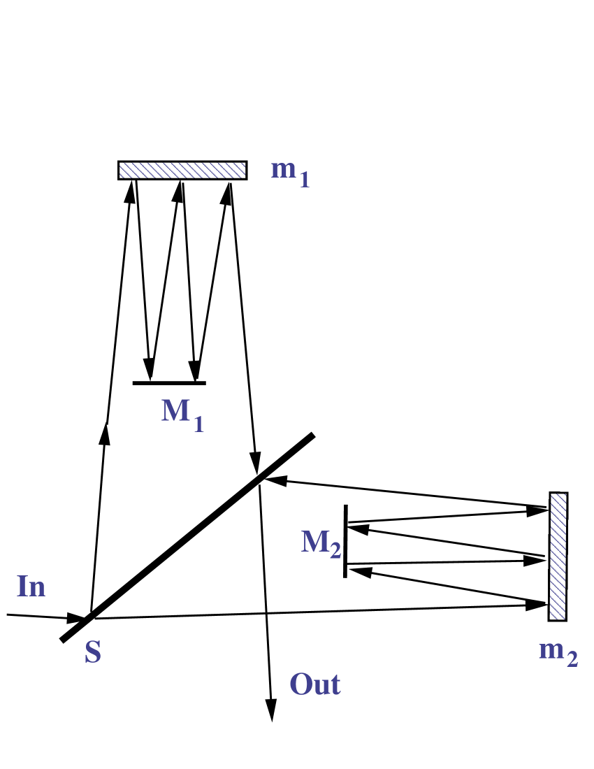
FIG. 1.: The essentials of a Michelson interferometer. An input laser beam (“In”) is split by the beam splitter S. The split beam bounces $b$ times (here $b=3$) in each arm between a free mass ($m_{1}$ or $m_{2}$) and a fixed mirror ($M_{1}$ or $M_{2}$) before being recombined to form the output beam (“Out”). The mirrors of interest for the radiation pressure fluctuations are located on the free masses.

A Position Uncertainty in the Photon Number Approach

In this subsection, we will review the conventional, photon number approach to calculating interferometer noise [1, 2]. The effect of multiple bounces is accounted for by multiplying the momentum operator in Eq. (14) by a factor 0f $b$

$$p=2b\omega n\,.$$ (86)

This introduces a factor of $b^{2}$ in the mean squared velocity fluctuation

$$\langle\Delta v^{2}\rangle=4b^{2}\frac{\omega A\rho}{m^{2}}\tau\,.$$ (87)

The root mean squared position uncertainty of each mirror due to radiation pressure fluctuations is then of order

$${\Delta x}_{rp}=b\frac{\sqrt{\omega P}}{m}\,\tau^{\frac{3}{2}}\,,$$ (88)

where $P=A\rho$ is the mean power in the laser beam. There is another source of noise in the interferometer, the photon counting error, also known as shot noise. This arises from the uncertainty in the location of an interference fringe when a finite number of photons are counted, and is of order

$${\Delta x}_{pc}=\frac{1}{2b\sqrt{\omega P\tau}}\,.$$ (89)

If we minimize the net squared position uncertainty

$$({\Delta x}_{rp})^{2}+({\Delta x}_{pc})^{2}$$ (90)

with respect to $P$, the result is the optimum power

$$P_{opt}=\frac{m}{2\omega\tau^{2}b^{2}}\,.$$ (91)

When $P=P_{opt}$, the position uncertainty becomes

$$\Delta x=\Delta x_{sql}=\sqrt{\frac{\tau}{m}}\,,$$ (92)

known as the standard quantum limit.

The standard quantum limit is the position uncertainty which one obtains after time $\tau$ by preparing a particle in a wavepacket state with initial spatial width $\Delta x_{0}$ and momentum spread $\Delta p=m\Delta x_{0}/\tau$. After time $\tau$ has elapsed, the spread in the width of the wavepacket, $\Delta p\,\tau/m$, is of the order of $\Delta x_{0}$. Thus the standard quantum limit can be interpreted as being the minimum position uncertainty which can be maintained for a time of the order of $\tau$.

B Position Uncertainty in the Stress Tensor Approach

Here we wish to look in more detail at how the position uncertainty arises in a description involving the quantum stress tensor. The position of each mass is disturbed by the pressure fluctuations, leading to an error in the measurement of the optical path length. The displacement of a given mass is described by the time integral of Eq. (19)

$$x-x(0)=\frac{1}{m}\int_{0}^{\tau}\int_{0}^{t}\int_{A}T_{xx}(x_{1})da_{1}dt_{1}dt$$ (93)

The dispersion in position is then given by an expression analogous to Eq. (20)

$$\langle\triangle x^{2}\rangle \equiv \langle x^{2}\rangle-\langle x\rangle^{2}$$ (94)

$$= \frac{1}{m^{2}}\int_{A}\int_{A}da_{1}da_{2}\int_{0}^{\tau}\int_{0}^{\tau}dt\,dt^{\prime}\int_{0}^{t}\int_{0}^{t^{\prime}}\left[\langle:T_{xx}(x_{1})::T_{xx}(x_{2}):\rangle\right.$$ (95)

$$- \left.\langle:T_{xx}(x_{1}):\rangle\langle:T_{xx}(x_{2}):\rangle\right]dt_{1}dt_{2}\,.$$ (96)

As before, only the cross term in the stress tensor fluctuations will contribute when the quantum state is a coherent state. If we use this fact, and then take the second derivative with respect to $\tau$, we can write

$$\frac{d^{2}}{d\tau^{2}}\langle\triangle x^{2}\rangle = \frac{2}{m^{2}}\left[\int_{0}^{\tau}dt_{1}\int_{0}^{\tau}dt_{2}\int da_{1}\int da_{2}\langle T_{xx}(t_{1})T_{xx}(t_{2})\rangle_{cross}\right.$$ (98)

$$\left.+\int_{0}^{\tau}dt^{\prime}\int_{0}^{t^{\prime}}dt_{2}\int da_{1}\int da_{2}\langle T_{xx}(\tau)T_{xx}(t_{2})\rangle_{cross}\right]\,.$$

Now we need to assume that the laser beam is switched on in the past and then switched off in the future. This issue was discussed in Ref. [3], where integrations by parts were performed in order to deal with the singular behavior of the cross term. The asymptotic condition insures that the surface terms arising in the integrations all vanishes. In the present calculation, we require that the normal ordered factors vanish at $t=\tau$, and hence the second term on the right hand side of Eq. (98) vanishes. The remaining term is proportional to $\langle\triangle v^{2}\rangle$, so that

$$\frac{d^{2}}{d\tau^{2}}\langle\triangle x^{2}\rangle=2\,\langle\triangle v^{2}\rangle\,.$$ (99)

Thus if $\langle\triangle v^{2}\rangle\propto\tau$, then $\langle\triangle x^{2}\rangle\propto\tau^{3}$. This calculation is the justiication for Eq. (88).

There are two major issues to be studied in remainder of this section. One is to study the effects of multiple bounces within one arm of the interferometer, which will be done in the following subsection. The other is to study whether there are any correlations between the two arms. The discussion in Sect. IV A implicitly assumed the absence of correlations, and a justication for this assumption was given by Caves [1]. In the present context, there is a correlation term $\langle\triangle x_{12}^{2}\rangle$ which takes the form of Eq. (94) with $x_{1}$ on one mirror and $x_{2}$ on the other mirror. We will argue below in Sect. IV D 2 that this term is negligible compared to $\langle\triangle x^{2}\rangle$ for each arm separately.

C Multiple Bounces in One Arm

1 A Delay Line

Now we wish to consider the situation where a laser beam bounces several times between a pair of mirrors, as illustrated in Fig. 1. This arrangement is sometimes called a “delay line”. Suppose that the beam is recycled $b$ times within a single interferometer arm. We have already seen that in the photon number approach, the momentum fluctuation of the end mirror, $\langle\triangle p^{2}\rangle$ is now proportional to $b^{2}$. Specifically,

$$\langle\triangle p^{2}\rangle=b^{2}\,\langle\triangle p^{2}\rangle_{1}\,,$$ (100)

where $\langle\triangle p^{2}\rangle_{1}$ is the single bounce result given in Eq. (70). One can understand this result in the following way: if there is a fluctuation in the number of photon entering the interferometer arm, that fluctuation is maintained on each of the successive bounces. If slightly more than the expected number of photons hit the mirror on the first bounce, the same excess will reappear on later bounces. One can picture the same photons as simply recycling $b$ times. However, in the stress tensor approach, it is less obvious how the $b^{2}$ factor will arise. This factor requires that the stress tensor fluctuations at the different spots on the mirror be exactly correlated with one another.

We can understand this by returning to Eq. (62). If the integrations run over all time and over the entire area of the mirror, then they pick up contributions from all of the bounces. Let us first suppose that the spots formed on succesive bounces overlap on the same region of the mirror. In this case, the mode function $u_{0}$ is approximately periodic for $b$ periods:

$$u_{0}(t,{\bf x})\approx u_{0}(t+2Ln,{\bf x})\,,\quad n=1,2,\cdots,b-1\,.$$ (101)

Let the first bounce occur at time $t=0$, and subsequent bounces at $t=2Ln$. More precisely, these are the mean times at which the wavepacket hits the mirror. Let $T$ be some time interval which is long compared to the length of the wavepacket, but short compared to $2L$. Equation (68) becomes

$$\langle\triangle p^{2}\rangle=|z|^{2}\,I^{2}\,,$$ (102)

where

$$I=\int_{-\infty}^{\infty}dt\int da\,u_{0}(x)u_{0}^{*}(x)=\sum_{n=0}^{b-1}\int_{2Ln-T}^{2Ln+T}dt\int da\,u_{0}(x)u_{0}^{*}(x)\,.$$ (103)

Note that the time intervals which are ignored in going from the first form to the second are ones in which $u_{0}=0$ on the mirror, that is, in between bounces. However, the periodicity property, Eq. (101), implies that each term in the sum is equal. Furthermore, each term gives the same contribution to $I$ as was found in the single bounce case:

$$I=b\int_{-T}^{T}dt\int da\,u_{0}(x)u_{0}^{*}(x)\,=2b\omega\,.$$ (104)

Thus we obtain Eq. (100).

Note that it does not matter whether the spots formed on the various bounces actually overlap on the mirror or not. If they do not, then Eq. (101) is replaced by a more complicated relation involving an offset in position for the different bounces. However, once the area integration is performed, this is irrelevant, and we still obtain Eq. (103). Note that we are assuming that on all bounces, the beam is nearly perpendiular to the mirror.

2 A Fabry-Perot Cavity

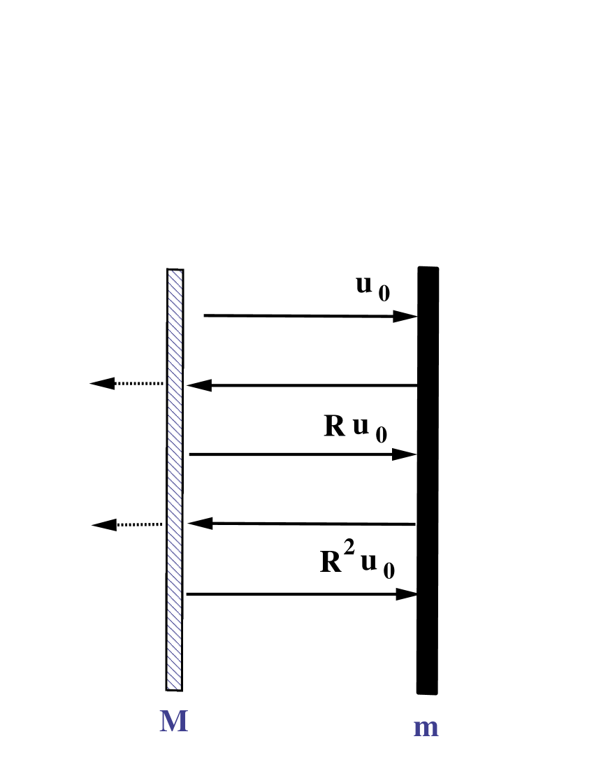
FIG. 2.: A Fabry-Perot cavity. Here the right mirror $m$ is perfectly reflecting, and the left mirror $M$ is partially reflecting, with a reflection amplitude $R$. An initial wavepacket $u_{0}$ returns to $m$ as $Ru_{0}$ on the first bounce, as $R^{2}u_{0}$ on the second bounce, ect.

The delay line arrangement sketched in Fig. 1 and discussed above implies a precise number of bounces. Another possibility, which is more likely to be used in actual interferometers, is the Fabry-Perot cavity, illustrated in Fig. 2. Here at least one of the mirrors is partially reflecting, leading to a finite storage time for a wavepacket in the cavity. We will discuss the case where the mirror on the free mass is assumed to be perfect, but the opposite mirror in the cavity is not. This assumption allows us to continue to use our previous expressions, especially Eq. (54). If the mirror on the free mass is not perfect, then it is necessary to modify this expression and include electric field terms as well.

Let $R$ be the complex reflection amplitude for the imperfect mirror, so that $|R|^{2}$ is the fraction of the power reflected on each bounce. We assume that once inside the cavity, a given wavepacket mode bounces an infinite number of times, but with diminishing amplitude. The effective number of bounces, $b^{\prime}$, can be defined by

$$|R|^{2b^{\prime}}=\frac{1}{2}\,.$$ (105)

Thus the energy stored in an occupied wavepacket mode is reduced by a factor of $\frac{1}{2}$ after $b^{\prime}$ bounces. We can then write

$$|R|^{2}=e^{-\frac{\ln 2}{b^{\prime}}}\approx 1-\frac{\ln 2}{b^{\prime}}\,,\quad b^{\prime}\gg 1\,.$$ (106)

The effect of the finite reflectivity of the left mirror is to introduce a factor of $r$ each time the wavepacket returns to the right mirror. Recall that the magnetic field mode $u_{0}$ has no phase shift upon reflection from the perfect mirror. We can express this as the following condition on the mode function:

$$u_{0}(t+2Ln,{\bf x})=R^{n}\,u_{0}(t,{\bf x}),\quad n=0,1,2,\cdots,\quad-T<t<T\,.$$ (107)

That is, $u_{0}(t,{\bf x})$ for $-T<t<T$ is the initial form of the wavepacket when it hits the left mirror for the first time. The above relation gives its form when it returns for the $n$-th time.

We can now use this relation to write the analog of Eq. (103):

$$I=\int_{-\infty}^{\infty}dt\int da\,u_{0}(x)u_{0}^{*}(x)=\sum_{n=0}^{\infty}\int_{-T}^{T}dt\int da\,R^{n}u_{0}\,{R^{*}}^{n}(x)u_{0}^{*}(x)=\frac{1}{1-|R|^{2}}\,I_{1}.$$ (108)

We can now combine this with Eq. (62) to write

$$\langle\triangle p^{2}\rangle=\left(\frac{b^{\prime}}{\ln 2}\right)^{2}\,\langle\triangle p^{2}\rangle_{1}\,,$$ (109)

This result is the analog of Eq. (100) for the case of a Fabry-Perot cavity. In both cases, the momentum fluctuations grow as the square of the effective number of bounces.

D The Equal Arm Interferometer

In an equal arm interferometer with a perfect (loss-free) 50-50 beam splitter, the input power is divided equally between the two arms. In the late 1970’s, there was a controversy over whether radiation pressure fluctuations will create noise in such an interferometer. The arguments reviewed at the beginning of this section leading to the standard quantum limit, Eq. (92), assume that the radiation pressure fluctuations in the two arms are uncorrelated. However, one would expect that a fluctuation which sends more power into one arm will cause a corresponding deficit in the other arm. This would lead to anticorrelated pressure fluctuations. Caves [1, 2] resolved this controversy in the context of the photon number approach. He showed that when vacuum modes which enter an unused port of the interferometer are included, the fluctuations are uncorrelated. In this subsection, we will rederive this result using the stress tensor approach.

1 Properties of a Beam Splitter

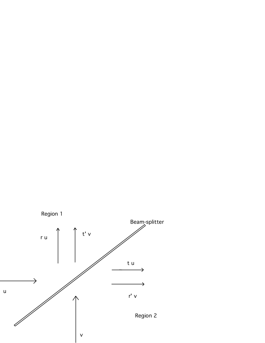
FIG. 3.: u and v represent the two incident wavepacket. $r\,,t$ are the complex amplitude reflectivity and transmissivity for incident light u, and $r^{\prime}\,,t^{\prime}$ are for the incident light v

Let us consider a perfect beam splitter. (See Fig. 3) It needs to satisfy the reciprocity relations, originally derived by Stokes in 1849,

$$|r|=|r^{\prime}|\,\,,\,\,|t|=|t^{\prime}|\,,$$ (110)

$$|r|^{2}+|t|^{2}=1$$ (111)

and

$$r^{\prime}\,t^{*}+r^{*}t^{\prime}=0\,,$$ (112)

where $r\,,t$ are the complex amplitude reflectivity and transmissivity for light incident from one side and $r^{\prime}\,,t^{\prime}$ for light from the other side. The first equation, Eq. (110), arises form the assumption that the reflectivity is the same from both sides. The other two equations are the results due to the additional assumption of a no-loss beam splitter. Assume that we send in a wavepacket $u_{0}$ into the beam splitter in the $x$ direction. Then it will reflect the amount $r\,u_{0}$ to region $1$ and transmit $t\,u_{0}$ to region $2$. If this is a no-loss beam splitter, then the inverse operation will bring the reflected and transmitted wavepackets back to the original incident wavepacket,

$$(r\,u_{0})r^{*}+(t\,u_{0})t^{*}=u_{0}\,,$$ (113)

which leads to Eq. (111). If there is another wavepacket $u_{1}$ coming into the beam splitter from the $y$ direction as well as the one $u_{0}$ from $x$, then in region $1$ we have the transmitted wavepacket $t^{\prime}\,u_{1}$ in additional to the reflected wavepacket $r\,u_{0}$, Similarly we get $t\,u_{0}+r^{\prime}\,u_{1}$ in the region $2$. Again the inverse operation yields the relations

$$(r\,u_{0}+t^{\prime}\,u_{1})r^{*}+(t\,u_{0}+r^{\prime}\,u_{1})t^{*}=u_{0}$$ (114)

and

$$(r\,u_{0}+t^{\prime}\,u_{1})t^{\prime*}+(t\,u_{0}+r^{\prime}\,u_{1})r^{\prime*}=u_{1}$$ (115)

for a no-loss, perfect beam splitter. Both equations here will lead to the reciprocity relation Eq. (112). For a $50-50$ beam splitter, $r^{\prime}=r$, $t^{\prime}=t$. Without losing generality, we may take the coefficients to be

$\displaystyle r=\frac{1}{\sqrt{2}}e^{i\,\phi_{r}\,}$and

$\displaystyle t=\frac{1}{\sqrt{2}}e^{i\,\phi_{t}\,,}$where $\phi_{r}\,,\phi_{t}$ are the phase change due to reflection and transmission, respectively. Plug them into the reciprocity relation Eq. (112), and the phase difference becomes

$$\triangle=\phi_{r}-\phi_{t}=\frac{n\pi}{2}\,\,,n=1,3,5...\,\,\,.$$ (116)

This phase difference is crucial in the discussion of the momentum correlation of the two end mirrors in interferometer.

2 Correlation between two arms

In a quantum mechanical treatment of the radiation field in the presence of a beam splitter, one often speaks of light entering one port of the interferometer and of vacuum entering the other, unused port [1, 2, 10]. From our point of view, this language is misleading. Vacuum modes are everywhere, and are entering both ports. Furthermore, there are an infinite number of such vacuum modes, and one would like to see more clearly which ones are actually relevant in a given situation.

Assume that wavepacket $u_{0}$ (the occupied mode) with a particular frequency is incident on the beam splitter. It will reflect $r\,u_{0}$ to mirror $\#1$ and transmit $t\,u_{0}$ to mirror $\#2$ (See Fig. 3). Similarly, at mirror $\#1$ there are modes $r\,u_{j}$ reflected from the vacuum fields coming from the input port and $t\,u_{k}$ transmitted from the vacuum fields coming from the output port. At mirror $\#2$, we have vacuum modes $t\,u_{j}$ and $r\,u_{k}$ in addition to the occupied mode, $t\,u_{0}$. If we consider the momentum difference transferred to the mirrors $p=p_{1}-p_{2}$, then the deviation becomes

$$\langle\triangle p^{2}\rangle=\langle\triangle p_{1}^{2}\rangle+\langle\triangle p_{2}^{2}\rangle-2\langle\triangle p_{1}\triangle p_{2}\rangle\,.$$ (117)

Now in arm $\#1$ the incident wavepacket is $r\,u_{0}$ and the complete set of wavepackets from vacuum are $(\sum_{j}r\,u_{j}+\sum_{k}t\,u_{k})$. Follow the reasoning leading to Eq. (62) in the one arm case; the momentum dispersion of mirror $\#1$ becomes

$$\langle\triangle p_{1}^{2}\rangle$$ (118)

$$= |z|^{2}Re[\int dt\int da\,r\,u_{0}(\sum_{j}r\,u_{j}+\sum_{k}t\,u_{k})^{*}\int dt^{\prime}\int da^{\prime}\,r^{*}u^{*}_{0}(\sum_{j}r\,u_{j}+\sum_{k}t\,u_{k})]$$ (119)

$$= |z|^{2}\left|\int dt\int da\,u_{0}u_{0}^{*}\right|^{2}*\frac{1}{4}Re[(1+e^{i\triangle})(1+e^{-i\triangle})]$$ (120)

$$= \frac{|z|^{2}}{2}\left|\int dt\int da\,u_{0}u_{0}^{*}\right|^{2}\,,$$ (121)

Here we used the result $\triangle=\frac{n\pi}{2}$ from Eq. (116). The momentum dispersion of mirror $\#2$, $\langle\triangle p_{2}^{2}\rangle$ will be the same as $\langle\triangle p_{1}^{2}\rangle$. The correlation between mirrors is

$$\langle\triangle p_{1}\triangle p_{2}\rangle$$ (122)

$$= |z|^{2}Re[\int dt\int da\,r\,u_{0}(\sum_{j}r\,u_{j}+\sum_{k}t\,u_{k})^{*}\int dt^{\prime}\int da^{\prime}\,t^{*}u^{*}_{0}(\sum_{j}t\,u_{j}+\sum_{k}r\,u_{k})]$$ (123)

$$= |z|^{2}|\int dt\int da\,u_{0}u_{0}^{*}|^{2}*\frac{1}{4}Re[(1+e^{i\triangle})(1+e^{i\triangle})]$$ (124)

$$= |z|^{2}|\int dt\int da\,u_{0}u_{0}^{*}|^{2}*\frac{1}{4}Re[\pm 2i]$$ (125)

$$= 0\,.$$ (126)

We can see that there is no correlation between arms. The fluctuations are totally independent to each other. The dispersion of the momentum difference becomes

$$\langle\triangle p^{2}\rangle=2\langle\triangle p_{1}^{2}\rangle=|z|^{2}\left(\int dt\int da\,u_{0}u_{0}^{*}\right)^{2}=4\langle n\rangle\omega^{2}\,.$$ (127)

For $b$ bounces, the dispersion is

$$\langle\triangle p^{2}\rangle_{b}=2b^{2}\langle\triangle p_{1}^{2}\rangle=4b^{2}\langle n\rangle\omega^{2}\,.$$ (128)

This confirms that Eq. (87) give the correct velocity dispersion of each end mirror in the interferometer.

V Discussion and Conclusions

In this paper, we have shown how quantum fluctuations of radiation pressure arise from fluctuations of the stress tensor operator. Our results are in agreement with those obtained previously using a photon number counting approach. In our approach, the radiation pressure fluctuations in a coherent state are due entirely to the cross term in the product of stress tensors. This term is both dependent upon the quantum state, and is singular in the limit of coincident points. however, we found that careful treatment of the integrals over space and time leads to a finite result.

The cross term can be interpreted as representing the interference between vacuum fluctuations and the real photons present. Thus radiation pressure fluctuations in the stress tensor approach are driven by vacuum fluctuations. It is useful to compare the photon number and stress tensor approaches at this point. Both approaches yield the same answers for all of the questions which were posed in this paper. (A possible exception is the Fabry-Perot cavity discussed in Sect. IV C 2 using only the stress tensor approach.) However, the conceptual pictures presented by the two approaches are quite different. In the photon number approach, the pressure fluctuations on a single mirror are attributed to statistical variations in the numbers of photons striking the mirror. However, when one wants to treat the problem of noise in an intererometer, especially the lack of correlation between the fluctuations in the two arms, it is necessary to invoke vacuum fluctuations [1, 2]. In our view, the stress tensor approach provides a more unified description in which the role of vacuum fluctuations is clear from the outset. It is also likely to generalize more easily to complex situations. For example, all of the treatments of radiation pressure fluctuations, with which we are aware, assume that the end mirrors are perfectly reflecting. However, the stress tensor approach could be easily adapted to account for the finite reflectivity of this mirror.

Radiation pressure fluctuations will play a role in laser interferometer detectors of gravity waves, especially in the future. At that point, it should become possible to measure these fluctuations experimentally. Confirmation of their existence can be viewed as experimental evidence for the reality of the cross term.

Of special significance is the role of radiation pressure fluctuations in understanding the fundamental physics of stress tensor fluctuations. It seems natural that the same principles which apply to the stress tensor as a source of pressure on a mirror should also apply to the stress tensor as a source of gravity. We have seen that the cross term is essential to understand radiation pressure fluctuations. It then follows that the cross term must be included in the treatment of spacetime metric fluctuations driven by stress tensor fluctuations.

Acknowledgement: We would like to thank K. Olum and C. M. Caves for valuable discussions. This work was supported in part by the National Science Foundation under Grant PHY-9800965.

Appendix

In this appendix, we calculate the integral $J$ defined in Eq. (37). Define $u=t_{1}-t_{2}$ and $v=t_{1}+t_{2}$. Next use the identities

$$\cos(\omega t_{1})\cos(\omega t_{2})=\frac{1}{2}[\cos(\omega u)+\cos(\omega v)]$$ (A1)

and

$$\int_{0}^{\tau}\int_{0}^{\tau}dt_{1}dt_{2}=\frac{1}{2}\left(\int_{-\tau}^{0}du\int_{-u}^{u+2\tau}dv+\int_{0}^{\tau}du\int_{u}^{2\tau-u}dv\right)\,.$$ (A2)

After evaluation of the $v$-integrations, we may write

$$J=\int_{0}^{\tau}du\,\frac{(\tau-u)(u^{2}+a)}{(u^{2}-b^{2})^{3}}\,\cos{\omega u}-\frac{1}{2\omega}\int_{0}^{\tau}du\,\frac{u^{2}+a}{(u^{2}-b^{2})^{3}}\,[\sin{\omega u}+\sin\omega(u-2\tau)]\,.$$ (A3)

The second integral in the above expression approaches a constant as $\tau\rightarrow\infty$, whereas the first integral contributes a linearly growing term:

$$J\sim\tau\int_{0}^{\infty}du\,\frac{u^{2}+a}{(u^{2}-b^{2})^{3}}\,\cos{\omega u}=\frac{1}{2}\tau\int_{-\infty}^{\infty}du\,\frac{u^{2}+a}{(u^{2}-b^{2})^{3}}\,\cos{\omega u}\,.$$ (A4)

This integral contains third-order poles at $u=\pm b$. It can be expressed as

$$J=\frac{1}{4}\,\tau(J_{+}+J_{-})\,,$$ (A5)

where in $I_{+}$ we assume ${\textrm{Im}}\,b>0$ and in $I_{+}$ we take ${\textrm{Im}}\,b>0$. Each of these integrals is in turn expressed as

$$I_{\pm}=\frac{1}{2}(I_{\pm 1}+I_{\pm 2})\,,$$ (A6)

where

$$I_{\pm 1}=\int_{-\infty}^{\infty}du\,\frac{u^{2}+a}{(u^{2}-b^{2})^{3}}\,{\textrm{e}}^{i\omega u}$$ (A7)

and

$$I_{\pm 2}=\int_{-\infty}^{\infty}du\,\frac{u^{2}+a}{(u^{2}-b^{2})^{3}}\,{\textrm{e}}^{-i\omega u}\,.$$ (A8)

Each of these integrals is evaluated by closing the contour of integration in the appropriate half plane, and then evaluating the integral by a combination of integration by parts and Cauchy’s theorem. For example, in the case of $I_{+1}$, we close in the upper half plane and write

$$I_{+1} = \frac{1}{2}\int_{-\infty}^{\infty}du\,\left(\frac{d^{2}}{du^{2}}\;\frac{1}{u-b}\right)\,\frac{u^{2}+a}{(u+b)^{3}}\,{\textrm{e}}^{i\omega u}=\frac{1}{2}\int_{-\infty}^{\infty}du\,\frac{1}{u-b}\,\frac{d^{2}}{du^{2}}\left[\frac{u^{2}+a}{(u+b)^{3}}\,{\textrm{e}}^{i\omega u}\right]$$ (A9)

$$= \pi i\left\{\frac{d^{2}}{du^{2}}\left[\frac{u^{2}+a}{(u+b)^{3}}\,{\textrm{e}}^{i\omega u}\right]\right\}_{u=b}\,.$$ (A10)

Similarly, we find

$$I_{+2}=-\pi i\left\{\frac{d^{2}}{du^{2}}\left[\frac{u^{2}+a}{(u-b)^{3}}\,{\textrm{e}}^{-i\omega u}\right]\right\}_{u=-b}\,,$$ (A11)

$$I_{-1}=-\pi i\left\{\frac{d^{2}}{du^{2}}\left[\frac{u^{2}+a}{(u+b)^{3}}\,{\textrm{e}}^{-i\omega u}\right]\right\}_{u=b}\,,$$ (A12)

and

$$I_{-2}=\pi i\left\{\frac{d^{2}}{du^{2}}\left[\frac{u^{2}+a}{(u-b)^{3}}\,{\textrm{e}}^{i\omega u}\right]\right\}_{u=-b}\,.$$ (A13)

We may now combine all of these results to obtain the expression for $J$, Eq. (40). Note that this calculation involves integrations by parts very similar to those used in Ref. [3] and illustrated in Sect. II of the present paper.

REFERENCES

- [1] C. M. Caves, Phy. Rev. Lett. 45, 75 (1980).
- [2] C. M. Caves, Phys. Rev. D 23, 1693 (1981).
- [3] C.-H. Wu and L.H. Ford, Phys. Rev. D 60, 104013 (1999), gr-qc/9905012.
- [4] L.H. Ford, Ann. Phys (NY) 144, 238 (1982).
- [5] S. del Campo and L.H. Ford, Phys. Rev. D 38, 3657 (1988).
- [6] C.-I Kuo and L.H. Ford, Phys. Rev. D 47, 4510 (1993), gr-qc/9304008.
- [7] N.G. Phillips and B.L. Hu, Phys. Rev. D 55, 6123 (1997), gr-qc/9611012.
- [8] K.T.R. Davies and R.W. Davies, Can. J. Phys. 67, 759 (1989); K.T.R. Davies, R.W. Davies, and G. D. White, J. Math. Phys. 31, 1356 (1990).
- [9] D.Z. Freedman, K. Johnson and J.I. Latorre, Nucl. Phys. B371, 353 (1992).
- [10] L. Mandel and E. Wolf, Optical Coherence and Quantum Optics (Cambridge University Press, London, 1995), Sect. 10.9.5 .