Luttinger model approach to interacting one–dimensional fermions in a harmonic trap

Abstract

A model of interacting one–dimensional fermions confined to a harmonic trap is proposed. The model is treated analytically to all orders of the coupling constant by a method analogous to that used for the Luttinger model. As a first application, the particle density is evaluated and the behavior of Friedel oscillations under the influence of interactions is studied. It is found that attractive interactions tend to suppress the Friedel oscillations while strong repulsive interactions enhance the Friedel oscillations significantly. The momentum distribution function and the relation of the model interaction to realistic pair interactions are also discussed.

I Introduction

The rapid progress in cooling and magnetic trapping technology [1, 2, 3, 4, 5, 6, 7] makes it conceivable to produce a neutral ultra–cold quantum gas of quasi one–dimensional degenerate fermions following the recent achievement in three spatial dimensions [8]. Some experimental aspects of such a quasi one–dimensional fermion gas are discussed in [9].

In three spatial dimensions, identical spin polarized fermions experience only a weak interaction because the s–wave scattering contribution from short ranged pair potentials is forbidden. Scattering processes involving higher angular momenta have energy thresholds and freeze out at temperatures below the Fermi temperature $T_{F}$ [10]. At zero temperature only a weak but long ranged dipole–dipole interaction [11, 12] remains.

This classification scheme does not apply to fermions in one spatial dimension. One can only state that a contact interaction has no effect. It is tempting to completely neglect all interactions and treat the one–dimensional fermion system as an ideal gas in a harmonic trap. Some exact single particle properties of this system were given in [13, 9]. The theory of Luttinger liquids [14, 15, 16, 17, 18] (for reviews cf. [19, 20, 21]) suggests, however, that even weak interactions destroy the Fermi liquid picture in one spatial dimension. This holds also true for bounded Luttinger liquids [22, 23, 24, 25, 26, 27, 28] which display algebraically decaying correlations. The confining potential for the cases studied so far is provided by hard walls. In ultra–cold quantum gases a harmonic confining potential is more appropriate.

Besides the Luttinger approach to confined one–dimensional fermions, a wealth of exact results exist for the Calogero–Sutherland model [29, 30] with harmonic confinement and its extensions (cf., e.g., [31]). These results hold for the $1/r^{2}$ pair interaction. A recent path integral approach to the thermodynamics of harmonically confined fermions [32] assumes a harmonic pair interaction. A different treatment of that model is given in [33] and includes results for Green’s functions of one-dimensional fermions. The present approach, which is expected to be asymptotically correct for large fermion numbers, is more flexible with respect to the form of the interaction.

The method proposed is a transcription of the elementary solution of the Luttinger model (cf., e.g., [21]) to the present problem. It requires, however, a different bosonization scheme which we adopt from [34].

As a first application, we calculate the particle density. The particle density depends perturbationally on the interaction strength. But we are still able to present some interesting interaction effects related to the Friedel [35] oscillations.

The paper is organized as follows: In Sec. 2, we present the basic arguments of our approach. Sec. 3 discusses the occupation probabilities of single particle states and the corresponding particle density for two interaction models. Sec. 4 shortly discusses the momentum distribution function and its relation to the particle density. In an Appendix, the pertinent question of the relation between the model interaction and realistic interactions is studied and estimates of their respective strengths are made.

II Luttinger Approach

We consider a gas of spinless identical fermions in one spatial dimension and trapped in a harmonic potential

$$V(z)=\frac{1}{2}m\omega^{2}_{\ell}z^{2}.$$ (1)

The Hamiltonian in second quantization but without interactions is

$$\hat{H}_{0}=\sum^{\infty}_{n=0}\hbar\omega_{n}\,\hat{c}^{+}_{n}\hat{c}_{n},$$ (2)

with one–particle energies

$$\hbar\omega_{n}=\hbar\omega_{\ell}(n+1/2),\,\,\,n=0,1,....$$ (3)

The fermion creation operators $\hat{c}^{+}$ and destruction operators $\hat{c}$ obey the fermionic algebra $\hat{c}_{m}\hat{c}_{n}^{+}+\hat{c}_{n}^{+}\hat{c}_{m}=\delta_{m,n}$. This ensures that each (non-degenerate) energy level $\epsilon_{n}=\hbar\omega_{n}$ with (real) single particle wave function

$$\psi_{n}(z)=\sqrt{\frac{\alpha}{2^{n}n!\pi^{1/2}}}\,e^{-\alpha^{2}z^{2}/2}\,H_{n}(\alpha z)$$ (4)

is at most singly occupied. The intrinsic length scale of the system is the oscillator length $l=\alpha^{-1}$ where $\alpha$ is defined by $\alpha^{2}=m\omega_{\ell}/\hbar$. $H_{n}$ denotes a Hermite polynomial.

The spatial extension of the bounded system of $N$ fermions is measured by the Fermi width $L_{F}$, i.e., half the extension of the classically allowed region at the Fermi energy:

$$L_{F}=\frac{1}{\alpha}\sqrt{2N-1}\equiv L_{n=N-1}.$$ (5)

The Fermi energy itself is given by:

$$\epsilon_{F}=\hbar\omega_{\ell}(N-1)+\frac{1}{2}\hbar\omega_{\ell}=\hbar\omega_{\ell}(N-\frac{1}{2}),$$ (6)

with an associated Fermi wave number [36, 9]

$$k_{F}\equiv\alpha\sqrt{2N-1}\equiv\sqrt{2m\epsilon_{F}/\hbar^{2}}.$$ (7)

The density oscillations well inside the trap can be identified [9] as Friedel oscillations [35] with wave number $2k_{F}$.

As is seen from eq. (3), the single particle energies depend linearly on the quantum number $n$. A linear dispersion is one of the requirements which allow the treatment of the Luttinger model. Another requirement is the presence of an anomalous vacuum with linear dispersion extending to arbitrary negative energies. In our case, these fictitious free states belong to $n<0$. Formally, they have wave functions $\psi_{p}(z)\propto{\cal{D}}_{p}\left(\sqrt{2}\alpha z\right)$ with $p=-n<0$, ($n$: positive integer, ${\cal{D}}$: parabolic cylinder function) which do not belong to the Hilbert space. This deficiency is likely to have no effect because these functions are still normalizable in any finite spatial region $[-L,L]$ with $L\gg L_{F}$ to which all finite range interaction effects are confined. Furthermore, one expects that for sufficiently large fermion number $N$ the presence of the anomalous vacuum is harmless for processes near the Fermi energy $\epsilon_{F}\propto N$ [18].

Exploiting the presence of the anomalous vacuum, it is easy to show that the density fluctuation operators

$$\hat{\rho}(m)\equiv\sum_{p}\hat{c}^{+}_{p+m}\hat{c}_{p}$$ (8)

obey bosonic commutation relations

$$[\hat{\rho}(-p),\hat{\rho}(q)]=p\,\delta_{p,q}$$ (9)

for all integers $p$ and $q$. The bosonic operators defined according to

$$\hat{\rho}(p)=\left\{\begin{array}[]{lll}\sqrt{|p|}&\hat{d}_{|p|},&p<0,\\ \sqrt{p}&\hat{d}^{+}_{p},&p>0,\end{array}\right.$$ (12)

thus satisfy canonical commutation relations:

$$[\hat{d}_{m},\hat{d}^{+}_{n}]=\delta_{m,n}$$ (13)

for positive integers $m$ and $n$. The following argument is taken over from the Luttinger model: Since the free Hamiltonian $\hat{H}_{0}$ has the same commutators with $\hat{\rho}(p)$:

$$[\hat{H}_{0},\hat{\rho}(p)]=\hbar\omega_{\ell}\,p\,\hat{\rho}(p),$$ (14)

as

$$\tilde{H}_{0}=\hbar\omega_{\ell}\sum_{m>0}m\,\hat{d}^{+}_{m}\hat{d}_{m}$$ (15)

has with the corresponding $\hat{d}_{m}$ and $\hat{d}^{+}_{n}$, the low energy (density wave) excitations of the fermionic Hamiltonian can as well be described in the bosonic Hilbert space.

The form of the admissible four–fermion interaction in the full Hamiltonian is dictated by the requirement that it can be expressed in terms of density fluctuation operators. This restricts the form of the matrix elements of the interaction operator

$$\hat{V}=\frac{1}{2}\sum_{mnpq}V(m,p;q,n)\,(\hat{c}^{+}_{m}\hat{c}_{q})(\hat{c}^{+}_{p}\hat{c}_{n}).$$ (16)

Two solvable forms were found: The matrix elements

$$V(m,p;q,n)=\int_{-\infty}^{\infty}d1d2d3d4\,\psi_{m}(1)\psi_{p}(2)V(1,2;3,4)\psi_{q}(3)\psi_{n}(4)$$ (17)

must simplify according to

a)

$$V(m,p;q,n)=V_{a}(|q-m|)\,\delta_{m-q,n-p}\,,$$ (18)

which leads to

$$\hat{V}_{4}=\frac{1}{2}\sum_{m>0}V_{a}(m)\,m\left\{\hat{d}^{+}_{m}\hat{d}_{m}+\hat{d}_{m}\hat{d}^{+}_{m}\right\},$$ (19)

and

b)

$$V(m,p;q,n)=V_{b}(|q-m|)\,\delta_{q-m,n-p}\,,$$ (20)

which gives

$$\hat{V}_{2}=\frac{1}{2}\sum_{m>0}V_{b}(m)\,m\left\{\hat{d}^{2}_{m}+\hat{d}^{+2}_{m}\right\}.$$ (21)

$V_{a}(m)$ and $V_{b}(m)$ correspond to the $g_{4}$ and $g_{2}$ coupling functions of the Luttinger model. The Appendix discusses the relation of the present interactions to realistic four–fermion interactions.

The total bosonic interaction operator, which is added to the free Hamiltonian (15), thus is

$$\hat{V}=\frac{1}{2}\sum_{m>0}mV_{b}(m)\left\{\hat{d}^{+2}_{m}+\hat{d}^{2}_{m}\right\}+\frac{1}{2}\sum_{m>0}mV_{a}(m)\left\{\hat{d}^{+}_{m}\hat{d}_{m}+\hat{d}_{m}\hat{d}^{+}_{m}\right\}.$$ (22)

It is diagonalized in the bosonic Hilbert space by the Bogoliubov transformation

$$\tilde{H}=\tilde{H}_{0}+\hat{V}=\sum_{m>0}m\,\epsilon_{m}\hat{f}^{+}_{m}\hat{f}_{m}+\mbox{const.},$$ (23)

with the unitary operator

$$\hat{S}=\exp\left\{\frac{1}{2}\sum_{m>0}\zeta_{m}\left(\hat{f}^{2}_{m}-\hat{f}^{+2}_{m}\right)\right\}.$$ (24)

This transformation relates the $\hat{d}$–operators to new canonical $\hat{f}$–operators according to

$$\hat{d}_{m}=\hat{S}^{+}\hat{f}_{m}\hat{S}=\hat{f}_{m}\cosh\zeta_{m}-\hat{f}^{+}_{m}\sinh\zeta_{m}.$$ (25)

The transformation parameters $\zeta_{m}$ are given by

$$\tanh 2\zeta_{m}=\frac{V_{b}(m)}{\hbar\omega_{\ell}+V_{a}(m)}.$$ (26)

They depend also on the sign of the interactions. The spectrum of the density wave excitations is found to be

$$\epsilon_{m}=\sqrt{\left(\hbar\omega_{\ell}+V_{a}(m)\right)^{2}-V^{2}_{b}(m)}\equiv\left(\hbar\omega_{\ell}+V_{a}(m)\right)\cosh 2\zeta_{m}-V_{b}(m)\sinh 2\zeta_{m}.$$ (27)

It is also seen that $V_{a}(m)\neq 0$ only renormalizes the single particle energy $\hbar\omega_{\ell}$. For large $N$ and at the Fermi edge, a local pair potential contributes equally to $V_{a}(m)$ and $V_{b}(m)$ because of its symmetry $m\leftrightarrow q$ or $n\leftrightarrow p$ (see Appendix).

The matrix elements $V_{a}$ and $V_{b}$ determine a set of coupling constants

$$\gamma_{m}\equiv\sinh^{2}\zeta_{m}=\frac{1}{4}\left(K_{m}+\frac{1}{K_{m}}-2\right)\geq 0,$$ (28)

where $K_{m}$ is given by

$$K_{m}=\sqrt{\frac{\hbar\omega_{\ell}+V_{a}(m)-V_{b}(m)}{\hbar\omega_{\ell}+V_{a}(m)+V_{b}(m)}}=\exp(-2\zeta_{m}).$$ (29)

This is in complete analogy to the Luttinger model. There is an obvious consistency condition

$$|V_{b}(m)|\leq|\hbar\omega_{\ell}+V_{a}(m)|,$$ (30)

and a more subtle stability condition [18]:

$$\sqrt{m}\,\frac{V_{b}(m)}{\hbar\omega_{\ell}+V_{a}(m)}\stackrel{{\scriptstyle m\rightarrow\infty}}{{\longrightarrow}}0.$$ (31)

We will mostly assume $V_{a}(m)=V_{b}(m)\equiv V(m)$. Then the simple relations

$$\epsilon_{m}=\frac{\hbar\omega_{\ell}}{K_{m}},\quad V(m)=\frac{1}{2}\,\left(\frac{1}{K_{m}^{2}}-1\right)\,\hbar\omega_{\ell}$$ (32)

hold. We will also consider two specific interaction models:

• A toy model, called IM1, which is defined by $V(m)=V(1)(\delta_{m,1}+\delta_{m,-1})$ with a real amplitude $V(1)$.

• The analogue of the usual Luttinger liquid interaction with a small exponential decay in the coupling constants $\gamma_{m}$ according to $\gamma_{m}=\exp(-r_{\gamma}m)\,\gamma_{0}$ in order to satisfy (31). In the particle density considered below, further coupling constants $\alpha_{m}$ (cf. (42)) appear. For these coupling constants we assume a decay according to $\alpha_{m}=\exp(-r_{\alpha}m/2)\,\alpha_{0}$ with $\alpha_{0}=sgn(V(1))\sqrt{\gamma_{0}(1+\gamma_{0})}$. We call this model IM2. This model is not fully consistent because the exponential decay of $\gamma_{m}$ induces a non–exponential decay of $\alpha_{m}$ unless $\gamma_{0}\ll 1$ or $\gamma_{0}\gg 1$ when $r_{\alpha}\rightarrow r_{\gamma}$ or $r_{\alpha}\rightarrow 2r_{\gamma}$, respectively. By choosing $r_{\alpha}$ properly, it is possible to restrict the error. The choice $r_{\gamma}=r_{\alpha}\propto\sqrt{N^{-1}}$, which corresponds to the length scale $L_{F}$, also poses no problem when $N$ is large.

An essential step in the applicability of the Luttinger model is the correspondence between fermionic creation and destruction operators and exponents of bosonic fields involving the $\hat{d}$ (or $\hat{f}$)–operators [17, 18, 19, 20, 21]. The standard form of this bosonization is apparently not applicable to the present case. Instead we will use a method initially introduced in [34]. The authors define an auxiliary field according to

$$\hat{\psi}_{a}(v)\equiv\sum^{\infty}_{l=-\infty}e^{ilv}\hat{c}_{l}=\hat{\psi}_{a}(v+2\pi),$$ (33)

and prove the bosonization formula for the bilinear combination

$$\hat{\psi}^{+}_{a}(u)\hat{\psi}_{a}(v)=G_{N}(u-v)\exp\left\{-i\left(\hat{\phi}^{+}(u)-\hat{\phi}^{+}(v)\right)\right\}\exp\left\{-i\left(\hat{\phi}(u)-\hat{\phi}(v)\right)\right\},$$ (34)

involving the non–Hermitian bosonic field

$$\hat{\phi}^{+}(v)=i\sum^{\infty}_{n=1}\frac{1}{\sqrt{n}}e^{-inv}\hat{d}^{+}_{n}\neq\hat{\phi}(v),$$ (35)

and the Fermi sum

$$\quad G_{N}(u)=\sum^{N-1}_{l=-\infty}e^{-il(u+i\epsilon)}.$$ (36)

Equations (23), (25), (27), and (33) to (36) provide a framework for the calculation of the fermion density and also of correlation functions of the density for one–dimensional fermions in a harmonic trap interacting via (22). They do not, however, allow to calculate the time dependence in the single particle Green’s function.

In the remaining part we apply the concept to the fermion density in the trap.

III Perturbed Particle Density

The fermion density is given by the expectation value

$$n(z)=\langle\hat{\psi}^{+}(z)\hat{\psi}(z)\rangle.$$ (37)

Decomposing the fermionic destruction operator $\hat{\psi}(z)$ according to

$$\hat{\psi}(z)\equiv\sum^{\infty}_{m=0}\psi_{m}(z)\,\hat{c}_{m},$$ (38)

gives

$$n(z)=\sum^{\infty}_{m,n=0}\psi_{m}(z)\psi_{n}(z)\,\langle\hat{c}^{+}_{m}\hat{c}_{n}\rangle.$$ (39)

Thus, the computation of the expectation values $\langle\hat{c}^{+}_{m}\hat{c}_{n}\rangle$ is required. They become non–diagonal in the presence of interactions. Using the prescription of the last section, we find

$$\langle\hat{c}^{+}_{m}\hat{c}_{n}\rangle=\sum_{l=-\infty}^{N-1}\int^{2\pi}_{0}\int^{2\pi}_{0}\,\frac{dudv}{4\pi^{2}}\,e^{i(m-l)(u+i\epsilon)-i(n-l)(v-i\epsilon)}\,\,\langle e^{-i\hat{\phi}^{+}(u)+i\hat{\phi}^{+}(v)}e^{-i\hat{\phi}(u)+i\hat{\phi}(v)}\rangle.$$ (40)

By standard methods (bosonic Wick theorem $\langle\exp[\hat{A}]\rangle=\exp[\langle\hat{A}^{2}\rangle/2]$ for any linear combination $\hat{A}$ of $\hat{f}_{m}$ and $\hat{f}_{n}^{+}$) and at zero temperature (when $\langle\hat{f}_{m}\hat{f}_{n}^{+}\rangle=\delta_{m,n}$), the expectation value $\langle\quad\rangle\equiv\exp[-W]$ is calculated from

$$W=W(u,v)=2\sum^{\infty}_{m=1}\frac{1}{m}\,\left[\gamma_{m}-\alpha_{m}\,\cos m(u+v)\right]\left\{1-\cos m(u-v)\right\},$$ (41)

with

$$\alpha_{m}\equiv sgn(V(m))\sqrt{\gamma_{m}(1+\gamma_{m})}.$$ (42)

In this way, a reduction to ”quadratures” is achieved but nontrivial summations and integrations remain.

$W$ is a real and an even function of its arguments. This gives the symmetries

$$\langle\hat{c}^{+}_{m}\hat{c}_{n}\rangle=\langle\hat{c}^{+}_{n}\hat{c}_{m}\rangle=\langle\hat{c}^{+}_{m}\hat{c}_{n}\rangle^{*}.$$ (43)

It will also turn out that $\langle\hat{c}^{+}_{m}\hat{c}_{n}\rangle$ vanishes unless $|m-n|$ is even. The particle density thus admits the representation:

$$n(z,N,T=0)=\sum^{\infty}_{M=0}\psi_{M}(z)^{2}\,\langle\hat{c}^{+}_{M}\hat{c}_{M}\rangle+2\sum^{\infty}_{M=1}\sum_{p=1}^{M}\psi_{M-p}(z)\,\psi_{M+p}(z)\,\langle\hat{c}^{+}_{M-p}\hat{c}_{M+p}\rangle.$$ (44)

The $l$–summation in (40) can be performed and the two integrations appropriately transformed using the $2\pi$–periodicity of the integrand in (40).

Turning to the interaction model IM1, one of the integrations can be performed, giving

$$\langle\hat{c}^{+}_{M-p}\hat{c}_{M+p}\rangle=\frac{1}{2}\,\delta_{p,0}-\frac{1}{2\pi}\int_{-\pi}^{\pi}ds\, \left\{\frac{\sin((M+1/2-N)s)}{2\sin(s/2)}\right\}$$ (46)

$$\exp[-2\gamma_{1}(1-\cos(s))]\,I_{p}(2\alpha_{1}(1-\cos(s))).$$

Evidently, the factor in curly brackets, which stems from the $l$–summation, provides particle–hole symmetry: For $p\neq 0$ it has the form

$$\langle\hat{c}^{+}_{2N-1-M-p}\hat{c}_{2N-1-M+p}\rangle=-\langle\hat{c}^{+}_{M-p}\hat{c}_{M+p}\rangle,$$ (47)

i.e., in a plot of $\langle\hat{c}^{+}_{M-p}\hat{c}_{M+p}\rangle$ versus $M$ the point $(N-1/2,0)$ is the point of inversion symmetry. For $p=0$ one obtains the occupation numbers $\langle\hat{c}^{+}_{M}\hat{c}_{M}\rangle$, which satisfy

$$\langle\hat{c}^{+}_{2N-1-M}\hat{c}_{2N-1M}\rangle=1-\langle\hat{c}^{+}_{M}\hat{c}_{M}\rangle.$$ (48)

In the present fermionic case, they can be interpreted as occupation probabilities $P(M)$ of the single particle state $\psi_{m}$. The occupation probabilities show the expected smearing of the Fermi edge around $M=N-1$ due to interactions. The inversion symmetry point for the probabilities is $(N-1/2,1/2)$.

Several statements concerning (46) can be made:

• The result of first order many body perturbation theory in fermionic Hilbert space are exactly reproduced for $V_{a}(1)=0$ by expanding (46) to first order in the coupling constant $V_{b}(1)$ (i.e., $\gamma_{1}\rightarrow 0$, $\alpha_{1}\rightarrow\zeta_{1}\rightarrow V_{b}(1)/(2\hbar\omega_{\ell})$) [37].

• The results of direct numerical diagonalization of the perturbed fermionic Hamiltonian agree with the numerical evaluation of (46) up to $|\alpha_{0}|=1$ and for particle numbers $N$ of the order of $10$, the range investigated so far [38].

• The sum rule

  $$\int_{\infty}^{\infty}\,dz\,n(z,N,T=0)=\sum_{M=0}^{\infty}\,\langle\hat{c}^{+}_{M}\hat{c}_{M}\rangle=N$$ (49)

  is exactly obeyed by (46): Summing the expression in curly brackets in (46) from $M=0$ to $Q\gg N$ leads to the result $2\pi\delta(s)((Q+1)/2-N)$.

Returning to the particle density, the modification of $P(M)$ and the appearance of non–diagonal contributions has pronounced effects: For increasingly negative values of $\alpha_{1}$ the Friedel oscillations are diminished while positive $\alpha_{1}$ increase their amplitude. This will be even more pronounced in the interaction model IM2 in which several basic interactions are superimposed.

The corresponding formula for $\langle\hat{c}^{+}_{M-p}\hat{c}_{M+p}\rangle$ is more complicated and can be given in the form:

$$\langle\hat{c}^{+}_{M-p}\hat{c}_{M+p}\rangle=\frac{1}{2}\,\delta_{p,0}- \int^{\pi}_{-\pi}\frac{dt}{2\pi}\,\frac{\cos(p\,t)}{[1+Z_{\alpha}-\cos(t)]^{\alpha_{0}}}$$ (52)

$$\int^{\pi}_{-\pi}\frac{ds}{2\pi}\,\left\{\frac{\sin((M+1/2-N)s)}{2\sin(s/2))}\right\}\left(\frac{Z_{\gamma}}{[1+Z_{\gamma}-\cos(s)]}\right)^{\gamma_{0}}$$

$$\quad\quad\quad\,\,[(1+Z_{\alpha}-\cos(t-s))(1+Z_{\alpha}-\cos(t+s))]^{\alpha_{0}/2}.$$

The quantities $Z_{\gamma}$ and $Z_{\alpha}$ result from the decay functions of the coupling constants $\gamma_{m}$ and $\alpha_{m}$. They are given by

$$Z_{\gamma}=\cosh(r_{\gamma})-1,\quad Z_{\alpha}=\cosh(r_{\alpha}/2)-1.$$ (53)

Again, the sum rule (49) is strictly fulfilled.

Figure 1 shows the corresponding particle density for $\alpha_{0}=\pm 1$, $r_{\gamma}=0.3$, and $r_{\alpha}=0.4$ obtained by numerical integration of (52) and by summing the series (44) up to $M=2N=20$. The occupation probabilities are smoothed out and more spectral weight is found above the Fermi energy. Correspondingly, the particle density outside the classical region is enhanced. Most startling, however, is the strong enhancement of the Friedel oscillations in case of strong repulsive interaction and their nearly complete suppression for strong attractive interactions.

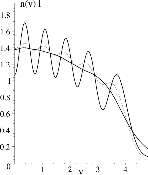
FIG. 1.: Dimensionless particle density $n$ in units of the inverse of the oscillator length $l$ versus dimensionless distance $v=z/l$ from the center of the one–dimensional harmonic trap for $N=10$ interacting spinless fermions at zero temperature. Broken curve shows unperturbed Friedel oscillations. Strongly oscillating curve refers to a repulsive interaction with $\alpha_{0}=1$ while the smooth curve is for an attractive interaction with $\alpha_{0}=-1$. Interaction model 2 has been used.

A discussion of the strength of the Friedel oscillations in a realistic quasi one-dimensional Fermi gas with interactions is addressed at the end of the Appendix.

IV One–Particle Momentum Distributions

Even for a confined system it makes sense to study the momentum density

$$p(k)\equiv\langle\hat{c}^{+}_{k}\hat{c}_{k}\rangle.$$ (54)

The operator $\hat{c}_{k}$ annihilates a fermion with (continuous) momentum $\hbar k$. It can be decomposed into the fermionic annihilation operators of the harmonic oscillator according to (A.5).

Taking into account that the expectation values $\langle\hat{c}^{+}_{m}\hat{c}_{n}\rangle$ vanish unless $|m-n|$ is even, the momentum density becomes

$$p(k) = \sum_{m,n=0}^{\infty}(f_{m}^{k})^{*}f_{n}^{k}\,(-1)^{m+n}\,\langle\hat{c}^{+}_{m}\hat{c}_{n}\rangle$$ (55)

$$= \frac{1}{\alpha^{2}}\,\sum_{m=0}^{\infty}\sum_{p=-m}^{m}(-1)^{p}\psi_{m-p}(\frac{k}{\alpha^{2}})\psi_{m+p}(\frac{k}{\alpha^{2}})\,\langle\hat{c}^{+}_{m-p}\hat{c}_{m+p}\rangle.$$ (56)

Obviously, the momentum distribution always satisfies the sum rule

$$\int_{-\infty}^{\infty}dk\,p(k)=N.$$ (57)

If the expectation values (52) were diagonal, as in the non–interacting case, one would obtain the relation

$$p(k)\equiv\frac{1}{\alpha^{2}}\,n(z=k/\alpha^{2}).$$ (58)

However, the non-diagonal matrix elements are relevant: From (46) it is seen that in case of IM1 the matrix elements obey the relation $\langle\hat{c}^{+}_{M-p}\hat{c}_{M+p}\rangle(-\alpha_{1})=(-1)^{p}\langle\hat{c}^{+}_{M-p}\hat{c}_{M+p}\rangle(\alpha_{1})$ leading to the remarkable result

$$p(k,\alpha_{1})=\frac{1}{\alpha^{2}}\,n(z=k/\alpha^{2},-\alpha_{1}),$$ (59)

for IM1, i.e., the momentum distribution functions behaves oppositely to the density: Attractive interactions increase the oscillations (with period $\pi\alpha^{2}/k_{F}$), repulsive interactions decrease them. This effect is also found for IM2 though it is less pronounced than in the density [39].

V Summary

Using methods borrowed from the theory of the Luttinger model, we propose a scheme to treat interacting fermions in a one–dimensional harmonic trap analytically. As in the Luttinger model, the method rests on the linear dispersion of non–interacting fermion states which is extended to negative energies. A crucial step in the treatment is the correspondence between fermionic operators and exponentials of bosonic fields. This allows to study the fermion density distribution in the trap. A detailed investigation of the relation between the model interaction and realistic pair interactions is also given.

Acknowledgements: The author thanks G. Alber, S. N. Artemenko, F. Gleisberg, F. Lochmann, T. Pfau, U. Schlöder, W. Schleich, J. Voit, and C. Zimmermann for valuable discussions and Deutsche Forschungsgemeinschaft for financial support.

VI Appendix

The Appendix compiles a number of formulae relating a physical two–body interaction to the four fermion matrix element in (17). We assume a local and translation invariant pair interaction

$$V(z_{1},z_{2};z_{3},z_{4})=V(z_{1}-z_{2})\,\delta(z_{1}-z_{3})\,\delta(z_{2}-z_{4}),$$ (A.1)

and start from the representation of the interaction operator in the momentum basis:

$$\hat{V}=\frac{1}{4\pi}\int^{\infty}_{-\infty}\,dk_{1}\,dk\,dk^{\prime}\,\tilde{V}(k_{1})\hat{c}^{+}_{k+k_{1}}\hat{c}^{+}_{k^{\prime}-k_{1}}\hat{c}_{k^{\prime}}\hat{c}_{k}.$$ (A.2)

The Fourier transform of the interaction potential is

$$\tilde{V}(k)=\int^{\infty}_{-\infty}\,dz\,e^{ikz}\,V(z)=\tilde{V}(-k)=\tilde{V}^{*}(k),$$ (A.3)

and the exchange symmetry of the pair potential $V(z)=V(-z)$ has been utilized.

By rearranging the operators in (A.2), one finds

$$\hat{V}=\frac{1}{4\pi}\int^{\infty}_{-\infty}\,dk_{1}\,dk\,dk^{\prime}\,\tilde{V}(k_{1})\left(\hat{c}^{+}_{k+k_{1}}\hat{c}_{k}\right)\left(\hat{c}^{+}_{k^{\prime}-k_{1}}\hat{c}_{k^{\prime}}\right)-\frac{1}{2}\hat{N}V(z=0),$$ (A.4)

where $\hat{N}$ is the fermion number operator. The self–energy contribution in (A.4), which is finite for any reasonably regularized potential, will be omitted. We go from the momentum basis to the harmonic oscillator basis by means of

$$\hat{c}_{k}=\sum^{\infty}_{n=0}(-1)^{n}\,f^{k}_{n}\,\hat{c}_{n},$$ (A.5)

with [9]

$$f^{k}_{n}\equiv\frac{1}{\sqrt{2\pi}}\,\int^{\infty}_{-\infty}\,dz\,e^{ikz}\psi_{n}(z)=\frac{i^{n}}{\alpha}\psi_{n}(z=\frac{k}{\alpha^{2}}).$$ (A.6)

Thus the usual form for the matrix elements, as used in the interaction operator

$$\hat{V}=\frac{1}{2}\,\sum^{\infty}_{mnpq=0}V(m,p;q,n)\,(\hat{c}^{+}_{m}\hat{c}_{q})(\hat{c}^{+}_{p}\hat{c}_{n}),$$ (A.7)

namely

$$V(m,p;q,n)=\int^{\infty}_{-\infty}\,dz_{1}dz_{2}\,\psi_{m}(z_{1})\psi_{p}(z_{2})V(z_{1}-z_{2})\psi_{q}(z_{1})\psi_{n}(z_{2}),$$ (A.8)

(with the obvious symmetries $m\leftrightarrow q$, $n\leftrightarrow p$) takes on the less familiar form

$$V(m,p;q,n)=(-1)^{n+q}\frac{1}{2\pi}\int^{\infty}_{-\infty}\,dk_{1}\,dk\,dk^{\prime}\,\tilde{V}(k_{1})\left\{f_{m}^{k-k_{1}}f_{q}^{k}\right\}\left\{f_{p}^{k^{\prime}+k_{1}}f^{k^{\prime}}_{n}\right\}.$$ (A.9)

It can be further evaluated by performing the convolution in (A.9). By using the method described in [9], one obtains

$$V(m,p;q,n)=(-1)^{n+q}\,i^{m+n+p+q}\frac{1}{2\pi}\,\int^{\infty}_{-\infty}\,dk_{1}\,C_{mq}(k_{1})\tilde{V}(k_{1})C_{pn}(-k_{1}),$$ (A.10)

with ($q\geq m$ is assumed)

$$C_{mq}(k_{1}) \equiv \frac{1}{\alpha^{2}}\int^{\infty}_{-\infty}\,dk\,\psi_{m}\left(\frac{k-k_{1}}{\alpha^{2}}\right)\psi_{q}\left(\frac{k}{\alpha^{2}}\right)$$ (A.11)

$$= \sqrt{\frac{m!}{q!}}\,\left(\frac{k_{1}}{\alpha\sqrt{2}}\right)^{q-m}\exp\left[-\frac{k^{2}_{1}}{4\alpha^{2}}\right]\,L^{(q-m)}_{m}\left(\frac{k^{2}_{1}}{2\alpha^{2}}\right)=(-1)^{m+q}\,C_{qm}(k_{1}).$$ (A.12)

In order to eliminate a possible contact interaction in $V(z)$, we set

$$V_{\mbox{eff}}(k)\equiv\tilde{V}(k)-\tilde{V}(k=\infty),$$ (A.13)

to obtain the following exact expression for the matrix elements of the potential in the basis of oscillator states and for $q\geq m$, $n\geq p$:

$$V(m,p;q,n)=i^{m+n+p+q}\{(-1)^{q-p}+(-1)^{n-m}\}\sqrt{\frac{m!p!}{2\,n!q!}}\,\frac{\alpha}{2\pi}$$ (A.14)

$$\int_{0}^{\infty}dv\,e^{-v}v^{(q-m+n-p-1)/2}\,V_{\mbox{eff}}(k=\alpha\sqrt{2v})\,L_{m}^{(q-m)}(v)\,L_{p}^{(n-p)}(v).$$ (A.15)

These matrix elements are of particular importance for values of the indices $m$, $n$, etc., which correspond to wave functions near the Fermi level, i.e., $m\approx N$ etc.. Setting $q=m+Q$ and exploiting $m\gg Q$ (e.g., $Q\leq\sqrt{N})$, the asymptotic expansion [41] of the Laguerre polynomials can be applied:

$$L_{m}^{(Q)}(v)\sim\left(\frac{m}{v}\right)^{\frac{Q}{2}}J_{Q}(2\sqrt{mv}).$$ (A.16)

This formula implies the approximation $(m+Q)!\approx m^{Q}m!$. Setting $n=p+R$, one finds

$$V(m,p;m+Q,p+R)\sim i^{Q+R}\frac{(-1)^{Q}+(-1)^{R}}{\sqrt{2}}\,\frac{\alpha}{2\pi}\,$$ (A.18)

$$\int^{\infty}_{0}\frac{dv}{\sqrt{v}}\,e^{-v}\,V_{\mbox{eff}}\left(k=\alpha\sqrt{2v}\right)\,J_{Q}(2\sqrt{mv})\,J_{R}(2\sqrt{pv}).$$

The integration region near $v=0$ will contribute little to matrix elements with $Q>0$ and $R>0$ (the $Q=R=0$ case in (18,20) is irrelevant) provided $\tilde{V}(k)$ is bounded for small wave numbers $k$. In order to estimate these matrix elements, we can thus assume $v$ to be not less than of order unity and apply the asymptotic expansion of the Bessel functions $J$. This gives:

$$V(m,p;m+Q,p+R) \approx i^{Q+R}\frac{(-1)^{Q}+(-1)^{R}}{\sqrt{2}}\,\frac{\alpha}{\pi^{2}}\,\int^{\infty}_{a}\frac{du}{u}e^{-\frac{u^{2}}{4}}$$ (A.20)

$$\cos\left(u\sqrt{m}-\frac{Q}{2}\pi-\frac{\pi}{4}\right)V_{\mbox{eff}}\left(k=\frac{\alpha u}{\sqrt{2}}\right)\cos\left(u\sqrt{p}-\frac{R\pi}{2}-\frac{\pi}{4}\right),$$

where $a$ is of order unity. We choose $a=1$. Finally, setting $R=Q+\Delta R$, leads to

$$V(m,p;m+Q,p+Q+\Delta R) \approx\frac{\alpha}{\pi^{2}\sqrt{2}}\,\cos(\frac{\pi\Delta R}{2})\,\int^{\infty}_{1}\frac{du}{u}e^{-\frac{u^{2}}{4}}V{\mbox{eff}}(k=\frac{\alpha u}{\sqrt{2}})$$ (A.22)

$$\left\{\cos\left(u(\sqrt{m}-\sqrt{p})\right)+(-1)^{Q}\sin\left(u(\sqrt{m}+\sqrt{p})\right)\right\}.$$

Equation (A.22) admits the following discussion of the matrix elements:

• The matrix elements depend weakly on $m$ and $p$ in the ranges $|\Delta m|\equiv|m-N|<\sqrt{N}$ and $|\Delta p|\equiv|p-N|<\sqrt{N}$.

• Elements with $\Delta R=0$ are (nearly) independent of $Q<\sqrt{N}$ and all have the same sign: They are positive for repulsive interactions and negative in the opposite case.

• Varying $\Delta R$, produces alternating signs which weakens the effect of these matrix elements.

These are essentially the properties which justify the model interactions (18) and (20). In this connection, it should be mentioned that, as in Luttinger liquid theory, one does not need a faithful representation of the physical interaction [18, 40] to capture essential features of the interaction.

For a numerical evaluation of the interaction strength, we begin with the interaction of longitudinally aligned magnetic dipoles (cf. [11, 12]) in a quasi one–dimensional magnetic trap for which the effective (attractive) potential is

$$V(z)=-\frac{\mu_{0}}{2\pi}\mu^{2}\frac{1}{(z^{2}+d^{2})^{3/2}}.$$ (A.23)

Here, an ultra–violet cut off has been introduced. It is given by the width of the one–dimensional channel, i.e., $d=\alpha_{t}^{-1}$, where $\alpha_{t}$ is the reciprocal harmonic oscillator length of the transverse (ground state) wave function. This length is large on an atomic scale. Introducing the ratio $\lambda\equiv\omega_{l}/\omega_{t}$, one has $d=\sqrt{\lambda}/\alpha$. In case of a completely filled one–dimensional trap, which we henceforth assume, $N=1/\lambda$ holds.

Fourier transforming the potential (A.23), gives

$$\tilde{V}(k)=V_{0}(\sqrt{\lambda}\,\frac{k}{\alpha})K_{1}(\sqrt{\lambda}\,\frac{k}{\alpha}).$$ (A.24)

This expression involves a modified Bessel function and is bounded (though not analytic) at $k=0$. It vanishes for large momenta. The prefactor contains the magnetic moment $\mu$ of the fermions and reads:

$$V_{0}=-\frac{\mu_{0}}{\pi}\,\frac{\mu^{2}\alpha^{2}}{\lambda}.$$ (A.25)

For IM1, the quantity

$$V(1)\approx\left[V_{0}\frac{\alpha}{\pi^{2}\sqrt{2}}\right]\,\int^{\infty}_{1}\,du\,\{\sqrt{\frac{\lambda}{2}}\,K_{1}(u\sqrt{\frac{\lambda}{2}})\}\,\exp\{-\frac{u^{2}}{4}\}\,\cos\left(u(\sqrt{m}-\sqrt{p})\right)$$ (A.26)

is needed. The contribution from the second term in (A.22) containing $\sqrt{m}+\sqrt{p}$ is negligible. The factor in square brackets can be written as

$$\left[V_{0}\frac{\alpha}{\pi^{2}\sqrt{2}}\right]=-\frac{1}{\sqrt{2}}\left(\frac{\mu_{0}\mu^{2}m_{A}\alpha N}{\pi^{3}\hbar^{2}}\right)\,\hbar\omega_{\ell},$$ (A.27)

where $m_{A}$ is the atom mass. The prefactor of the scaling energy $\hbar\omega_{\ell}$ is estimated for ${}^{6}Li$ to be $-3\cdot 10^{-3}(N/10^{4})$ adopting the data from [9]. The remaining integral in (A.26) is about unity for $|m-p|<\sqrt{N}$. So it needs about $N=10^{6}$ atoms in the trap to produce a significant effect of the dipole–dipole interaction.

For scattering processes in three dimensions, the van der Waals potential is more relevant. The dilute atoms in the trap (mean distance larger than 100 Bohr radii) explore mostly the long–range part of it. Reducing the $R^{-6}$ potential to an effective potential in one dimension, gives:

$$V(z)=-\frac{A}{(z^{2}+d^{2})^{3}},$$ (A.28)

with the Fourier transform

$$\tilde{V}(k)=-\frac{\pi}{8}\frac{A}{d^{5}}\,e^{-kd}\,(3+3kd+k^{2}d^{2}).$$ (A.29)

Following [42, 43], the coefficient $A$ can be expressed in terms of the coefficient $C_{6}$ therein, giving

$$V(1)\approx\left[\left(\frac{C_{6}}{16\pi\sqrt{2}}\right)\,e_{0}^{2}\,a_{0}^{5}\,\alpha_{t}^{5}\,\alpha\right]\, \hbar\omega_{\ell}\,\int^{\infty}_{1}\,\frac{du}{u}\,\exp(-u^{2}/4-u\sqrt{\lambda/2})$$ (A.31)

$$\left(3+3u\sqrt{\lambda/2}+u^{2}\lambda/2\right)\,\,\cos\left(u(\sqrt{m}-\sqrt{p})\right),$$

where $e_{0}$ and $a_{0}$ are electron charge and Bohr radius, respectively. Fixing $\omega_{\ell}$ at $2\pi\cdot 10s^{-1}$, as in [9], the evaluation of (A.31) gives a total prefactor of $\hbar\omega_{\ell}$ according to $\approx-6\cdot 10^{-7}\,(N/10^{4})^{5/2}$. Even for $N=10^{6}$, this is small compared to the dipole–dipole interaction. This reversal in the importance of the two interactions can be traced back to the ultra–violet cutoff $d\equiv\alpha_{t}^{-1}$ needed in the quasi one–dimensional forms of the interactions.

The choice of transverse cut-off determines the strength of the effective one-dimensional interaction. Our choice is motivated by the following fact: The transverse trap direction is associated with only one intrinsic length scale $(L_{F})_{t}=1/\alpha_{t}=l_{t}=l\sqrt{\lambda}\approx 1/k_{F}$ and this length coincides with the shortest intrinsic length scale of the longitudinal trap direction.

The amplitude of the Friedel oscillations inside a bounded Fermi sea scales with the particle number $N$ as $1/N$. Adopting the numbers estimated above, it is impossible to detect Friedel oscillations in a gas of $10^{6}$ ${}^{6}Li$ atoms with present techniques. However, the interaction strength $V(1)$ between magnetic dipoles scales as $\mu^{2}m_{A}^{3/2}$. Using ${}^{53}Cr$ instead of ${}^{6}Li$ enhances the interaction by nearly three orders of magnitude. Fermionic molecules are even more promising, especially when they are polar (cf., e.g., [44]): An electric dipole moment of 1 Debye ($p=a_{0}e_{0}/2.5$) leads to an interaction strength which is enhanced by a factor $(0.8/\alpha_{S})^{2}\approx 10^{5}$ ($\alpha_{S}$: fine structure constant) over that from magnetic dipoles of magnitude $\mu_{B}$ ($\mu_{B}$: Bohr’s magneton).

Thus it seems that the issue of Friedel oscillations in an interacting quasi one-dimensional degenerate Fermi gas is not purely academic.

REFERENCES

• [1] C. G. Townsend, N. H. Edwards, C. J. Cooper, K. P. Zetie, C. J. Foot, A. M. Steane, P. Szriftgiser, H. Perrin, and J. Dalibard, Phys. Rev. A 52 1423 (1995).
• [2] O. J. Luiten, M. W. Reynolds, and J. T. M. Walraven, Phys. Rev. A 53, 381 (1996).
• [3] V. Vuletic, T. Fischer, M. Praeger, T. W. Hänsch, and C. Zimmermann, Phys. Rev. Lett. 80, 1634 (1998).
• [4] J. Fortagh, A. Grossmann, C. Zimmermann, and T. W. Hänsch, Phys. Rev. Lett. 81, 5310 (1999).
• [5] J. Denschlag, D. Cassettari, and J. Schmiedmayer, Phys. Rev. Lett. 82, 2014 (1999).
• [6] J. H. Thywissen, M. Olshanii, G. Zabow, M. Drndic, K. S. Johnson, R. M. Westervelt, and M. Prentiss, Eur. Phys. J. D7, 361 (1999).
• [7] J. Reichel, W. Hänsel, and T. W. Hänsch, Phys. Rev. Lett. 83, 3398 (1999).
• [8] B. DeMarco and D. S. Jin, Science 285, 1703 (1999).
• [9] F. Gleisberg, W. Wonneberger, U. Schlöder, and C. Zimmermann, Phys. Rev. A 62, 063602 (2000).
• [10] B. DeMarco, J. L. Bohn, J. P. Burke, Jr., M. Holland, and D. S. Jin, Phys. Rev. Lett. 82, 4208 (1999).
• [11] K. Goral, K. Rzazewski, and T. Pfau, Phys. Rev. A 61, 051601(R) (2000).
• [12] K. Goral, B-G. Englert, and K. Rzazewski, Phys. Rev. A 63, 033606 (2001).
• [13] P. Vignolo, A. Minguzzi, and M. P. Tosi, Phys. Rev. Lett. 85, 2850 (2000).
• [14] S. Tomonaga, Prog. Theor. Phys. 5, 544 (1950).
• [15] J. M. Luttinger, J. Math. Phys. 4, 1154 (1963).
• [16] D. C. Mattis and E. H. Lieb, J. Math. Phys. 6, 304 (1965).
• [17] A. Luther and I. Peschel, Phys. Rev. B 9 2911 (1974).
• [18] F. D. M. Haldane, J. Phys. C14, 2585 (1981).
• [19] V. J. Emery, Theory of the One-Dimensional Electron Gas, in Highly Conducting One-Dimensional Solids, edited by J. T. Devreese, R. P. Evard, and V. E. van Doren (Plenum, New York, 1979), p247.
• [20] J. Voit, Rep. Prog. Phys. 58, 977 (1995).
• [21] H. J. Schulz Fermi Liquids and Non-Fermi Liquids, in Mesoscopic Quantum Physics, edited by E. Akkermans, G. Montambaux, J.-L. Pichard, and J. Zinn-Justin (Elsevier, Amsterdam, 1995), p533.
• [22] J. L. Cardy, J. Phys. A 17, L385 (1984).
• [23] S. Eggert and I. Affleck, Phys. Rev. B 46, 10866 (1992).
• [24] M. Fabrizio and A. O. Gogolin, Phys. Rev. B 51, 17827 (1995).
• [25] R. Egger and H. Grabert, Phys. Rev. Lett. 75, 3505 (1995).
• [26] Y. Wang, J. Voit, and Fu-Cho Pu, Phys. Rev. B 54, 8491 (1996).
• [27] A. E. Mattsson, S. Eggert, and H. Johannesson, Phys. Rev. B 56, 15615 (1997).
• [28] J. Voit, Yupeng Wang, and M. Grioni, Phys. Rev. B 61, 7930 (2000).
• [29] F. Calogero, J. Math. Phys. 10, 2197 (1969).
• [30] B. Sutherland, J. Math. Phys. 12, 246 (1971), Phys. Rev. A 4, 2019 (19971), Phys. Rev. A 5, 1372 (1972).
• [31] Norio Kawakami and Yoshio Kuramoto, Phys. Rev. B 50, 4664 (1994).
• [32] F. Brosens, J. T. Devreese, and L. F. Lemmens, Phys. Rev. E 57, 3871 (1998).
• [33] M. A. Zaluska-Kotur, M. Gajda, A. Orlowski, and J. Mostowski, Phys. Rev. A 61, 033613 (2000).
• [34] K. Schönhammer and V. Meden, Am. J. Phys. 64, 1168 (1996).
• [35] J. Friedel, Nuovo Cimento Suppl. 7, 287 (1958).
• [36] D. A. Butts and D. S. Rokhsar, Phys. Rev. A 55, 4346 (1997).
• [37] F. Gleisberg, private communication.
• [38] F. Lochmann, Diploma Thesis, University of Ulm, February 2001, unpublished.
• [39] An approximate analytical evaluation of (52) is possible for negative $\alpha_{0}$. By setting $s=0$ in the last factor of the integrand in (52), the integration over $t$ becomes trivial, giving $\delta_{p,0}$, i.e., the matrix elements become diagonal. The integration over $s$ leads to hypergeometric functions in two variables which are difficult to discuss.This approximation to the matrix elements is reasonable for calculating the density in the attractive case. However, the contributions of the (small) non-diagonal matrix elements to the momentum distribution interfere constructively enhancing the oscillations.
• [40] V. Meden, Phys. Rev. B 60, 4571 (1999).
• [41] M. Abramowitz and I. A. Stegun, Handbook of Mathematical Functions, (Dover, New York, 1970), equ. (22.15.2).
• [42] W. T. Zemke and W. C. Stwalley, J. Phys. Chem. 97, 2053 (1993).
• [43] R. Cote, A. Dalgarno, and M. J. Jamieson, Phys. Rev. A 50, 399 (1994).
• [44] H. L. Bethlem, G. Berden, F. M. H. Crompvoets, R. T. Jongma, A. J. A. van Roij, and G. Meijer, Nature (London) 406, 491 (2000).