Induced measures in the space of mixed quantum states

Abstract

We analyze several product measures in the space of mixed quantum states. In particular we study measures induced by the operation of partial tracing. The natural, rotationally invariant measure on the set of all pure states of a $N\times K$ composite system, induces a unique measure in the space of $N\times N$ mixed states (or in the space of $K\times K$ mixed states, if the reduction takes place with respect to the first subsystem). For $K=N$ the induced measure is equal to the Hilbert-Schmidt measure, which is shown to coincide with the measure induced by singular values of non-Hermitian random Gaussian matrices pertaining to the Ginibre ensemble. We compute several averages with respect to this measure and show that the mean entanglement of $N\times N$ pure states behaves as ln$N-1/2$.

e-mail: karol@cft.edu.pl    sommers@next30.theo-phys.uni-essen.de

I Introduction

Recent developments in the emerging field of quantum information increased an interest in investigation of the properties of the set of density matrices of a finite size. To characterize quantitatively properties of typical density matrices it is necessary to define a certain measure $\mu$ in this set, which will enable one to compute the desired averages over all $N\times N$ density matrices with respect to this measure. Only having chosen the measure $\mu$ it makes sense to ask about the probability to find a random density matrix representing an entangled state or to compute the average entanglement of mixed quantum states [1, 2, 3]. Alternatively one may search for a statistical ensemble of density matrices which corresponds to minimal prior knowledge about a quantum system [4, 5].

In the space of pure states of an $N$ dimensional Hilbert space ${\cal H}_{N}$, isomorphic with the complex projective space ${\mathbb{C}}P^{N-1}$, there exist a unique ’natural’ measure, $P_{N}(|\phi\rangle)$, induced by the Haar measure on the unitary group $U(N)$. In other words, the random pure state, defined by action of a random unitary matrix on an arbitrary reference state, $|\phi\rangle=U|\phi_{0}\rangle$, may be represented (in an arbitrary basis) as a certain row (or column) of the random matrix $U$. The measure $P_{N}(|\phi\rangle)=P_{N}(U|\phi\rangle)$ in the space of pure states is thus distinguished by the rotational invariance of the Haar measure [6, 7, 8].

This property of the set of pure states may suggest that there exists a natural measure in the space of mixed quantum states ${\cal M}_{N}$, distinguished in an analogous way. However, this might not be the case: it is not at all simple to select a single measure in ${\cal M}_{N}$ and provide rational arguments for its superiority [6, 4, 2, 3]. Any density matrix $\varrho$ is Hermitian and may be diagonalised by an unitary matrix $U$. It is thus tempting to assume that the distributions of eigenvalues and eigenvectors of $\varrho$ are independent, so $\mu$ factorizes into a product measure $\Delta\times\nu$. For the measure $\nu$ on the unitary group, which determines the statistics of the eigenvectors forming $U$, one may take the unique Haar measure on $U(N)$. On the other hand, it is much more difficult to find convincing arguments, which allow one to pick out the unique measure $\Delta$ defined on the simplex of eigenvalues.

To consider a possibility of defining induced measures in the $(N^{2}-1)$ dimensional space ${\cal M}_{N}$ it is worth to discuss the procedure of purification. Any mixed state $\varrho$, acting on ${\cal H}_{N}$, may be purified by finding a pure state $|\Psi\rangle$ in the composite Hilbert space ${\cal H}_{N}\otimes{\cal H}_{N}$, such that $\varrho$ is given by the partial tracing over the auxiliary subsystem,

$$|\Psi\rangle\longrightarrow{\varrho}={\rm Tr}_{2}\Bigl{(}|\Psi\rangle\langle\Psi|\Bigr{)}\ .$$ (1)

In a loose sense the purification corresponds to treating any density matrix of size $N$ as a vector of size $N^{2}$. For a given $\varrho$ finding a corresponding pure state $|\Psi\rangle$ does not have a unique solution since

$$\varrho={\rm Tr}_{2}\Bigl{(}|\Psi\rangle\langle\Psi|\Bigr{)}={\rm Tr}_{2}\Bigl{(}|\Psi^{\prime}\rangle\langle\Psi^{\prime}|\Bigr{)}\quad\quad\quad{\rm where}\quad\quad\quad|\Psi^{\prime}\rangle=({\mathbb{I}}\otimes U_{2})|\Psi\rangle$$ (2)

where $U_{2}$ is an arbitrary unitary matrix of size $N$ acting locally on the auxiliary subsystem.

It is now simple to formulate the idea of the induced measure: we choose the natural measure $P_{N^{2}}(|\Psi\rangle)$ in the space of purified states, and look for the measure $P_{N,N}(\varrho)$ induced by the operation of partial tracing (1). This idea, put forward by Braunstein [9], was further developed by Hall [4]. He considered the ensemble of pure states in the $NK$ dimensional space ${\cal H}_{N}\otimes{\cal H}_{K}$ distributed according to the the natural measure $P_{NK}(|\Psi\rangle)$. The partial tracing over the variables of ${\cal H}_{K}$ defines uniquely the induced measure $P_{N,K}(\varrho)$ in the space of mixed states ${\cal M}_{N}$. Hall found explicitly the probability distributions $P_{2,K}(\varrho)$ and computed mean entropy averaged over these measures. The aim of this work is to extend his results providing the general formula for $P_{N,K}(\varrho)$. Moreover, we propose other methods of defining induced measures via the Hilbert-Schmidt space and establish a link between them.

The space of linear operators acting on ${\cal H}_{N}$, equipped with the scalar product $\langle A|B\rangle=$tr$A^{\dagger}B$, is called the Hilbert-Schmidt space, ${\cal H}_{HS}$. It has $N^{2}$ complex dimensions and may be represented by the algebra of complex matrices of size $N$. Any non-zero matrix $A$ may be projected into the space of density matrices by [10]

$$A\longrightarrow{\varrho}=\frac{AA^{\dagger}}{\mbox{tr}AA^{\dagger}}\ .$$ (3)

It is easy to see that $AA^{\dagger}$ is Hermitian and positive (strictly speaking, non-negative), while the rescaling by the norm assures the trace condition tr$\varrho$=1. Obviously one may consider an alternative, entirely equivalent projection $A\to\varrho^{\prime}={A^{\dagger}A}/{\mbox{tr}A^{\dagger}A}$, which agrees with (3) for normal $A$.

Two matrices $A$ and $A^{\prime}$ produce the same state $\varrho$, if there exist an unitary $V$, such that $A^{\prime}=AV$. An arbitrary measure $P(A)$ in the Hilbert-Schmidt space induces thus a certain measure in the space $\cal M$ of density matrices. The eigenvalues of $\varrho$ are equal to the rescaled squared singular values of matrix $A$, where $SV(A)=\sqrt{{\rm eig}(AA^{\dagger})}$ [11]. Note that the singular values of $A$ and $A^{\prime}$ are the same. For $P(A)$ one may take the measure of Ginibre ensemble of (non-Hermitian) random Gaussian matrices. In this paper we prove that the measure induced in this way is equal to $P_{N,N}(\varrho)$, which is also shown to coincide with the measure related to the Hilbert-Schmidt metric.

Our paper is organized as follows. In Section II we write down the natural measure in the space of pure states and provide a review of different measures used in the space of the density matrices. Section III is devoted to measures induced by partial tracing. In section IV we discuss possibilities of generalizing our results and provide certain families of measures in $\cal M$. The paper is concluded in section V.

II Measures in the space of density matrices

A Natural measure on the space of pure states

Before concentrating on the set ${\cal M}_{N}$ of the density matrices of size $N$, let us discuss the space of pure states. For concreteness we start our considerations with the four dimensional Hilbert space - the simplest case important from the point of view of quantum entanglement. The set of pure states of a $4$ dimensional Hilbert space forms a complex projective space ${\mathbb{C}}P^{3}$, on which the natural uniform measure exists. To generate random pure states according to such a measure on this $6$ dimensional manifold, we take a vector of a random unitary matrix distributed according to the Haar measure on $U(4)$. The Hurwitz parametrisation [12] gives

$$|\Psi\rangle=(\cos\vartheta_{3},\sin\vartheta_{3}\cos\vartheta_{2}e^{i\varphi_{3}},\sin\vartheta_{3}\sin\vartheta_{2}\cos\vartheta_{1}e^{i\varphi_{2}},\sin\vartheta_{3}\sin\vartheta_{2}\sin\vartheta_{1}e^{i\varphi_{1}}),$$ (4)

where $\vartheta_{k}\in[0,\pi/2],$ and $\varphi_{k}\in[0,2\pi)$ for $k=1,2,3$.

A uniform distribution over almost all of ${\mathbb{C}}P^{3}$ is obtained by choosing the uniform distribution of the ’polar’ angles; $P(\varphi_{k})=1/2\pi$. In analogy to the volume element on the sphere, the ’azimuthal’ angles $\vartheta_{k}$ should be taken in a nonuniform way, with the probability density [12]

$$P(\vartheta_{k})=k\sin(2\vartheta_{k})(\sin\vartheta_{k})^{2k-2}\quad\quad{\rm for}\quad\quad\vartheta_{k}\in[0,\pi/2],\quad\ \ k=1,2,3.$$ (5)

In practice it is convenient to use auxiliary independent random variables $\xi_{k}$ distributed uniformly in $[0,1]$ and to set $\vartheta_{k}={\rm arcsin}\bigl{(}\xi_{k}^{1/2k}\bigr{)}$. In order to generalize the parametrisation (4) for a vector belonging to the $N$-dimensional Hilbert space, one uses $(N-1)$ polar angles $\varphi_{k}$, uniformly distributed in $[0,2\pi)$, and $(N-1)$ independent azimuthal angles $\vartheta_{k}$, distributed according to (5) [13]. The volume element in space ${\mathbb{C}}P^{N-1}$ reads thus

$$dv=\prod_{k=1}^{N-1}\cos\vartheta_{k}(\sin\vartheta_{k})^{2k-1}d\vartheta_{k}d\varphi_{k},$$ (6)

while the total volume of the manifold of pure states

$$V_{N}=\prod_{k=1}^{N-1}\int_{0}^{\pi/2}\cos\vartheta_{k}(\sin\vartheta_{k})^{2k-1}d\vartheta_{k}\prod_{k=1}^{N-1}\int_{0}^{2\pi}d\varphi_{k}=\frac{\pi^{N-1}}{(N-1)!}$$ (7)

is proportional to the product of the volume of the $(N-1)$-d torus, (built of the phases $\varphi_{k}$), times the volume of the $(N-1)$-d simplex ${\cal S}_{N}$, (built of the angles $\vartheta_{k}$) [14]. The natural measure (6) in ${\mathbb{C}}P^{N-1}$ induces the uniform measure in the simplex ${\cal S}_{N}$ [3]. In appendix A we show that the same measure is given by squared absolute values of $N$ independent random complex Gaussian numbers $z_{i}$, rescaled as $|z_{i}|^{2}\to|z_{i}|^{2}/\sum_{i=1}^{N}|z_{i}|^{2}$. Thus a random pure state may be constructed of $N$ appropriately rescaled complex random numbers drawn according to the normal distribution.

It is worth to note that the natural measure (6) is compatible with the Fubini-Study metric on ${\mathbb{C}}P^{N-1}$, in the sense that the measure of a certain $\epsilon$-neighbourhood of any chosen point is the same [10]. The average value of some function of a state, $X_{\psi}=X(|\psi\rangle)$ (e.g. an observable $\langle X\rangle_{\psi}$), over the entire manifold of pure states is then defined as

$${\bar{X}}=\frac{1}{V_{N}}\int_{CP^{N-1}}X_{\psi}dv(|\psi\rangle).$$ (8)

B Product measures in the space of mixed states

Consider a Hermitian, nonnegative matrix $\varrho$ of size $N$, normalized as tr$\varrho=1$. It represents a mixed state belonging to the space ${\cal M}_{N}$ and may be diagonalized by a unitary rotation. Let $B$ be a diagonal unitary matrix. Since

$$\varrho=U\Lambda U^{\dagger}=UB\Lambda B^{\dagger}U^{\dagger},$$ (9)

the rotation matrix $U$ is determined up to $N$ arbitrary phases entering $B$. The number of irrelevant phases increases, if the spectrum of $\varrho$ is degenerated (see e.g. [15]). The total number of independent variables used to parametrize a density matrix $\varrho$ is equal to $N^{2}-1$, provided, no degeneracy occurs. In recent papers discussing the relative volume of the set of entangled states [1, 3], we considered the product measures

$$\mu=\Delta\times\nu.$$ (10)

The first factor defines a measure in the $(N-1)$ dimensional simplex of eigenvalues entering $\Lambda$, since due to the trace condition $\sum_{i=1}^{N}\lambda_{i}=1$. The measure $\nu$, defined in the space of unitary matrices $U(N)$, is responsible for the choice of eigenvectors of $\varrho$. It is natural to take for $\nu$ the Haar measure $\nu_{u}$ on $U(N)$, so that the probability distributions are rotationally invariant, $P(\varrho)=P(U\varrho U^{\dagger})$. On the other hand, as pointed out by Slater [2], there exist several possible choices for the measure $\Delta$.

C Measures induced by random vectors

In Ref. [3] we defined a unitary product measure by taking for the vector ${\vec{\Lambda}}=\{\lambda_{i}\}$ the squared moduli of complex elements of a column (say, the first column) of an auxiliary random unitary matrix $V$ drawn with respect to the Haar measure $\nu_{u}$ on $U(N)$

$$\lambda_{i}=|V_{i1}|^{2}.$$ (11)

The distribution $P_{u}({\vec{\Lambda}})$ obtained in this way is nothing else but the distribution of components of a random vector on ${\mathbb{C}}P^{N-1}$, uniform on the simplex of eigenvalues [3]. In a similar way one defines the orthogonal product measure where $\lambda_{i}=|O_{i1}|^{2}$ and $O$ is an orthogonal matrix drawn with respect to the Haar measure $\nu_{o}$ on $O(N)$.

Let us stress that the name of the product measure (orthogonal or unitary) is related to the distribution $\Delta$ on the simplex of eigenvalues, while the random rotations $U$ are always assumed to be distributed according to the Haar measure $\nu_{u}$ in $U(N)$. Thus both measures may be linked directly to the well known Gaussian unitary (orthogonal) ensembles of random matrices [16, 17], referred to as GUE and GOE. The measure $\mu_{o}$ is determined by squared components of a real eigenvector of a GOE matrix, while the measure $\mu_{u}$ may defined by components of a complex eigenvector of GUE matrices.

It is easy to see, that these measures on the simplex are special cases of the Dirichlet distribution [2]

$$\Delta_{s}(\lambda_{1},\dots,\lambda_{N-1})=\alpha_{s}\lambda_{1}^{s-1}\!\dots\!\lambda_{N-1}^{s-1}(1-\lambda_{1}-\!\dots\!-\lambda_{N-1})^{s-1}.$$ (12)

where $s>0$ is a free parameter and $\alpha_{s}$ stands for a normalization constant. The last component is determined by the trace condition $\lambda_{N}=1-\lambda_{1}-\dots-\lambda_{N-1}$. The uniform measure $\Delta_{1}$ describes the unitary measure $\mu_{u}=\Delta_{1}\times\nu_{u}$, while the case $s=1/2$ corresponds to the orthogonal measure, $\mu_{o}=\Delta_{1/2}\times\nu_{u}$ [3]. The latter is related to the Fisher information metric [19], the Mahalonobis distance [20] and Jeffreys’ prior [21].

It is instructive to consider the limiting cases of the distribution (12). For $s\to 0$ one obtains a singular distribution peaked at the pure states [2], while in the opposite limit $s\to\infty$, the distribution is concentrated on the maximally mixed state $\varrho_{*}$ described by the vector ${\vec{\Lambda}}=\{1/N,\dots,1/N\}$. Changing the continuous parameter $s$ one can thus control the average purity of the generated mixed states.

D Measures related to metrics

There exist several different distances in the space of mixed quantum states - (see e.g. [22, 23]). Each metric generates a measure, since one can assume that drawing random matrices from each ball of a fixed radius is equally likely. The balls are understood with respect to a given metric. We shall consider here two most important examples: the Hilbert-Schmidt metric and the Bures metric.

The Hilbert-Schmidt distance between any two density operators is given by the Frobenius (Hilbert-Schmidt) norm of their difference

$$D_{HS}(\varrho_{1},\varrho_{2})=\sqrt{{\rm Tr}[(\varrho_{1}-\varrho_{2})^{2}]}.$$ (13)

With respect to this metric the set of the two levels mixed states has the geometry of the Bloch sphere and its interior. For any dimension $N$ the infinitesimal distance takes a particularly simple form

$$(ds_{HS})^{2}={\rm Tr}[(\delta\varrho)^{2}]$$ (14)

and allows one to compute the volume element, normalize it by appropriate constants $C_{N}$ and to obtain the probability distribution

$$P_{HS}(\lambda_{1},\dots,\lambda_{N})=C_{N}\delta(1-\sum_{i=1}^{N}\lambda_{i})\prod_{j<k}^{N}(\lambda_{j}-\lambda_{k})^{2}.$$ (15)

This joint probability distribution, derived by Hall [4], defines the Hilbert-Schmidt measure $\Delta_{HS}$ in the space of diagonal matrices, and a product measure (10) in the space of density matrices.

Another measure is related with the Bures distance in the space of mixed quantum states, [24, 25],

$$D_{B}(\varrho_{1},\varrho_{2})=\sqrt{2\bigl{(}1-{\rm{tr}[(\varrho_{1}^{1/2}\varrho_{2}\varrho_{1}^{1/2})^{1/2}]\bigr{)}}},$$ (16)

It corresponds to the minimal Fubini-Study distance between all possible purifications (1) of both mixed states $\varrho_{1}$ and $\varrho_{2}$. With respect to this distance the $3$-dimensional set of $N=2$ density matrices exhibits the geometry of a half of the hypersphere $S^{3}\in R^{4}$, with pure states at the hyper-meridian [26].

The infinitesimal Bures distance between $\varrho$ and $\delta\varrho$ was found by Hübner [27]

$$(ds_{B})^{2}=\frac{1}{2}\sum_{j,k=1}^{N}\frac{|\langle j|\delta\varrho|k\rangle|^{2}}{\lambda_{j}+\lambda_{k}},$$ (17)

where $\lambda_{k}$ and $|k\rangle$ represent eigenvalues and eigenvectors of $\varrho$. Hall computed the corresponding volume element, and received the Bures probability distribution [4]

$$P_{B}(\lambda_{1},\dots,\lambda_{N})=C^{\prime}_{N}\frac{\delta(1-\sum_{i=1}^{N}\lambda_{i})}{(\lambda_{1}\cdots\lambda_{N})^{1/2}}\prod_{j<k}^{N}\frac{(\lambda_{j}-\lambda_{k})^{2}}{\lambda_{j}+\lambda_{k}}.$$ (18)

This measure was later analyzed by Slater [18], who found the normalization constants $C^{\prime}_{N}$ for $N=3,4$ and $5$ and together with Byrd analyzed the geometry induced by the Bures measure for $N=3$ [28]. The Bures measure is monotone, i.e. it does not increase under the action of completely positive, trace preserving maps [22].

E $N=2$: Measures in the Bloch ball

To experience some features of different measures consider the set of $2\times 2$ density matrices. Such a matrix can be expressed by the Pauli matrices ${\vec{\sigma}}$ as $\varrho=I/2+{\vec{\sigma}}\cdot{\vec{r}}$, where ${\vec{r}}$ is a three dimensional vector of modulus $r\leq 1/2$. Pure states correspond to the Bloch sphere, $r=1/2$, while the center of the ball, $r=0$, corresponds to the maximally mixed state proportional to the identity matrix. The eigenvalues of $\varrho$ read $\lambda_{1}=1/2+r$, and $\lambda_{2}=1/2-r$. The rotationally invariant Haar measure $\nu_{u}$ implies in this case the uniform distribution of the pure states on the Bloch sphere. The product measures may differ by a different radial distribution P(r).

The unitary measure $\Delta_{1}$ is uniform in radius, $P_{u}(r)=2$ for $r\in[0,1/2]$, while the orthogonal measure $\Delta_{1/2}$ defined by (12) gives the ”cosine distribution”, $P_{o}(r)=4/(\pi\sqrt{1-4r^{2}})$. The Hilbert-Schmidt measure (15) reads for $N=2$

$$P_{HS}(r)=24r^{2}\quad{\rm for}\quad r\in[0,1/2]$$ (19)

The quadratic factor relates to the Jacobian in $3$-D spherical coordinates, so the Hilbert-Schmidt measure corresponds to the uniform coverage of the entire Bloch ball [4].

On the other hand, the Bures measure (18) implies the following radial distribution, obtained by substituting $\lambda_{1}=1/2+r$ and $\lambda_{2}=1/2-r$

$$P_{B}(r)=\frac{32r^{2}}{\pi\sqrt{1-4r^{2}}}.$$ (20)

where $r\in[0,1/2]$. As shown in Fig. 1a this distribution is more concentrated on high purity states with large $r$, located close to the Bloch sphere.

To analyze the simplest measure $P_{2,2}(\varrho)$ induced by partial tracing, consider pure state $|\Psi\rangle=(x,y,z,t)$ of the $2\times 2=4$ dimensional Hilbert space ${\cal H}_{4}$. The corresponding density matrix reads

$\displaystyle\varrho=|\Psi\rangle\langle\Psi|=\left[\begin{array}[]{cccc}xx^{\ast}&xy^{\ast}&xz^{\ast}&xt^{\ast}\\ yx^{\ast}&yy^{\ast}&yz^{\ast}&yt^{\ast}\\ zx^{\ast}&zy^{\ast}&zz^{\ast}&zt^{\ast}\\ tx^{\ast}&ty^{\ast}&tz^{\ast}&tt^{\ast}\end{array}\right],$

Performing the partial tracing with respect to the second subsystem one gets the reduced density matrix

$$\varrho_{A}=Tr_{B}(\varrho)=\left[\begin{array}[]{cc}xx^{\ast}+yy^{\ast}&xz^{\ast}+yt^{\ast}\\ zx^{\ast}+ty^{\ast}&zz^{\ast}+tt^{\ast}\end{array}\right]=:\left[\begin{array}[]{cc}b&w\\ w^{\ast}&1-b\end{array}\right],$$ (21)

where $b=xx^{\ast}+yy^{\ast}$ and $w=xz^{\ast}+yt^{\ast}$. Its eigenvalues might be written as $\lambda_{1,2}=\frac{1}{2}\pm r$, where $r=\frac{1}{2}\sqrt{(1-2b)^{2}+4|w|^{2}}$ It has been already proved by Hall [4] that the induced distribution $P_{2,2}(r)=24r^{2}$ and coincides with the Hilbert-Schmidt measure (19). In the next section we demonstrate that this relation holds for arbitrary $N$.

The pure states $|\Psi\rangle\in{\cal H}_{4}$ may be represented by the Schmidt decomposition $|\Psi\rangle=\cos\alpha|00\rangle+\sin\alpha|11\rangle$, where $\{|00\rangle,|01\rangle,|10\rangle,|11\rangle\}$ denotes the standard basis in ${\cal H}_{4}$ and $\alpha\in[0,\pi/4]$. The corresponding eigenvalues of the reduced density matrix are $\lambda_{1}=\cos^{2}\alpha$ and $\lambda_{2}=\sin^{2}\alpha$, so Eq. (19) implies the following distribution for the Schmidt angle

$$P(\alpha)=3\cos(2\alpha)\sin(4\alpha).$$ (22)

For $2\times 2$ systems ($N=2$) all measures of pure states entanglement are equivalent and may be expressed as a function of the Schmidt angle. For example, the tangle reads [29] $\tau=4{\rm det}\rho_{A}=4\lambda_{1}\lambda_{2}=\sin^{2}(2\alpha)$, while concurence $C$ is equal to $\sqrt{\tau}=sin(2\alpha)$. Changing variables in (22) we obtain the distributions

$$P(\tau)=\frac{3}{2}\sqrt{1-\tau}\qquad{\rm and}\qquad P(C)=3C\sqrt{1-C^{2}}\ .$$ (23)

consistent with numerical results of Kendon et al. [30]. First moments of these distributions give the mean tangle $\langle\tau\rangle_{CP^{3}}=2/5$ and the mean concurrence $\langle C\rangle_{CP^{3}}=3\pi/16\approx 0.589049$, averaged in the sense of (8) over the natural measure on the space of $N=4$ pure states.

In a similar way it is straightforward to compute the mean entanglement $E$. It is just the mean von Neumann entropy, $H(\varrho)=-{\rm tr}\varrho\ln\varrho$, of the reduced density matrices [4]

$$\langle E\rangle_{CP^{3}}=\langle E\rangle_{HS}=\int_{0}^{1/2}[-r\ln r-(1-r)\ln(1-r)]24r^{2}dr=\frac{1}{3}.$$ (24)

In the natural units we use the maximal entanglement $E_{\rm max}=\ln 2$. If one expresses the entanglement $E$ in units of $\ln 2$ then $E_{\rm max}/\ln 2=1$ and the mean value reads $\langle E\rangle/\ln 2=1/(3\ln 2)\approx 0.480898$. For other orthogonal, unitary and Bures measures we obtain, respectively, $\langle E\rangle_{o}=2\ln 2-1\approx 0.386$, $\langle E\rangle_{u}=1/2$ and $\langle E\rangle_{B}=2\ln 2-7/6\approx 0.219$. In the same way we compute the mean inverse participation ratio $R=[{\rm tr}\varrho^{2}]^{-1}$ of the reduced matrices. This quantity may vary from $R=1$ (for pure states) to $R=N$ (for the maximally mixed state), and has an interpretation as the effective number of pure states in the mixture. For density matrices distributed according to H-S measure one has $R_{HS}=5/4$. Performing an analogous integral for the Bures measure we obtain $R_{B}=8/7$, which reveals high concentration of this measure on the states of higher purity - see Fig. 1a. On the other hand, for orthogonal and unitary measures we find $R_{o}=4/3$ and $R_{u}=3/2$.

FIG. 1.: Distribution of the eigenvalues of density matrices of size $N=2$: (a) unitary product measure (uniform distribution – dotted line), orthogonal product measure (”cosine distribution” plotted with dashed line), Hilbert-Schmidt measure (solid line parabola) and Bures measure (dash-dotted line); (b) measures $P_{2,K}$ induced by partial tracing; solid line represents H-S measure i.e. $K=2$, dashed line $K=3$, dash-dotted line $K=4$, dotted line $K=5$.

III Measures induced by partial tracing of composite systems

A Joint probability distribution

Consider a bipartite $N\times K$ composite quantum system. Pure states of this system $|\Psi\rangle$ may be represented by a vector $|\Psi_{j}\rangle=\{\Psi_{1},\dots,\Psi_{M}\}^{T}$, where $M=NK$ is the dimension of the composite Hilbert space ${\cal{H}}={\cal{H}}_{A}\otimes{\cal{H}}_{B}$. In view of the operation of partial tracing it is convenient to work in a product basis $|i\rangle\otimes|k\rangle$, where $|i\rangle\in{\cal H}_{A};i=1,\dots,N$ while $|k\rangle\in{\cal H}_{B};k=1,\dots,K$. A pure state $|\Psi\rangle$ is then represented by a rectangular complex matrix $\psi_{ik}$. The normalization condition, $\|\psi\|^{2}={\rm tr}\psi\psi^{\dagger}=1$, is the only constraint imposed on this matrix. The density matrix $\varrho$, acting on the composite Hilbert space $\cal H$, is represented in this basis by a matrix labeled by four indices, $\varrho_{ik,i^{\prime}k^{\prime}}=\langle i|\otimes\langle k|\varrho|k^{\prime}\rangle\otimes|i^{\prime}\rangle=\psi_{ik}{\psi_{i^{\prime}k^{\prime}}}^{*}$. The partial tracing with respect to the $K$ dimensional subspace ${\cal H}_{B}$ gives a reduced density matrix of size $N$

$$\varrho^{A}={\rm Tr}_{B}{\varrho}~{}~{}~{}{\rm where}~{}~{}~{}\varrho_{ij}^{A}=\sum_{k=1}^{K}\psi_{ik}{\psi_{jk}}^{*}\ ,$$ (25)

while a symmetric operation of partial tracing over the first subsystem leads to a reduced density matrix $\varrho^{B}={\rm Tr}_{A}{\varrho}$ of size $K$, where $\varrho^{B}_{kl}=\sum_{i=1}^{N}\psi_{ik}{\psi_{il}}^{*}$. The natural measure in the space of $M=KN$ dimensional pure states induces then the measure $P_{N,K}(\varrho)$ in the space of the reduced density matrices (25) of size $N$. Note that the problem of measures induced by partial tracing may be considered as a projection of the $(KN-1)$ dimensional simplex of eigenvalues ${\cal S}_{KN-1}$ into simplices of smaller dimensions ${\cal S}_{N-1}$ or ${\cal S}_{K-1}$.

Without loss of generality we assume $K\geq N$, then ${\varrho}^{A}$ is generically positive definite. In the opposite case $K<N$ the reduced density matrix ${\varrho}^{A}$ has $N-K$ zero eigenvalues, but the reduced matrix ${\varrho}^{B}$ of size $K$ is positive definite and has the same positive eigenvalues. In any case we are interested only in the distribution of the positive eigenvalues. Let us call the corresponding positive reduced density matrix again ${\varrho}=\psi\psi^{\dagger}$ where $\psi$ is now considered as a $N\times K$ matrix. First we calculate the distribution of matrix elements

$$P({\varrho})\propto\int[d\psi]\ \delta({\varrho}-\psi\psi^{\dagger})\ \delta({\rm Tr}\psi\psi^{\dagger}-1)$$ (26)

where the first delta function is a delta function of a Hermitian Matrix and in the second delta function ${\rm Tr}\psi\psi^{\dagger}$ may be substituted by ${\rm Tr}{\varrho}$. Since ${\varrho}$ is positive definite we can make a transformation

$$\psi=\sqrt{{\varrho}}\tilde{\psi},\ \ \ [d\psi]={\rm det}{\varrho}^{K}\ [d\tilde{\psi}]\ .$$ (27)

Note that $[d\psi]$ includes (alternating) factors $d\psi_{ik}$ and $d{\psi_{ik}}^{*}$. The matrix delta function may now be written as

$$\delta(\sqrt{{\varrho}}(1-\tilde{\psi}\tilde{\psi}^{\dagger})\sqrt{{\varrho}})\ =\ {\rm det}{\varrho}^{-N}\ \delta(1-{\tilde{\psi}}{\tilde{\psi}}^{\dagger})\ ,$$ (28)

where the first factor on the right hand side is the inverse Jacobian of the corresponding transformation. As the result the distribution of matrix elements is given by

$$P({{\varrho}})\propto\theta({{\varrho}})\ \delta({\rm Tr}{{\varrho}}-1)\ {\rm det}{{\varrho}}^{K-N},$$ (29)

where the theta function assures that ${\varrho}$ is positive definite. It is then easy to show by the methods of random matrix theory that the joint density of eigenvalues $\Lambda=\{\lambda_{1},\lambda_{2},\dots,\lambda_{N}\}$ of ${\varrho}$ is given by

$$P_{N,K}(\lambda_{1},\dots,\lambda_{N})=C_{N,K}\delta(1-\sum_{i}\lambda_{i})\prod_{i}\lambda_{i}^{K-N}\theta(\lambda_{i})\prod_{i<j}(\lambda_{i}-\lambda_{j})^{2}.$$ (30)

The square of the Vandermonde determinant results from integrating out the eigenvectors and the normalization constant ( see also (51)) may be expressed in terms of the Euler Gamma function $\Gamma(x)$

$$C_{N,K}=\frac{\Gamma(KN)}{\prod_{j=0}^{N-1}\Gamma(K-j)\Gamma(N-j+1)}$$ (31)

written here for $K\geq N$. Observe that for $K=N$ the measure $P_{N,N}$ induced by partial tracing of the pure states in ${\mathbb{C}}P^{N^{2}-1}$ coincides with the Hilbert-Schmidt measure (15), so $C_{N,N}=C_{N}$. Moreover, it equals to the probability distribution of squared singular values $\sigma_{i}^{2}$ of matrices pertaining to the normalized Ginibre ensemble of complex matrices $A$, where $\sigma_{i}$ are given by the square roots of non-negative eigenvalues of $AA^{\dagger}$. This is even valid if $A$ is a $N\times K$ matrix $(K\geq N)$. To clarify this point instead of starting from equation (26) we could have been started from a distribution

$$P({\varrho})\propto\int[d\psi]\ \delta({\varrho}-\psi\psi^{\dagger}/{{\rm Tr}\psi\psi^{\dagger}})\ \exp(-{\rm Tr}\psi\psi^{\dagger})$$ (32)

Introducing a delta function for $t={{\rm Tr}\psi\psi^{\dagger}}$ and rescaling $\psi$ with $\sqrt{t}$ we see that both distributions (26) and (32) are equivalent and given by (29). This follows also from the fact that $N^{2}$ complex elements of the random matrix $A$ of the Ginibre ensemble may be treated as a random vector distributed according to the natural measure on ${\mathbb{C}}P^{N^{2}-1}$ – see Appendix A.

In this way one may give a simple recipe to generate a random density matrix according to the HS measure and similarly the generalisation (29):

a) prepare a square complex random matrix $A$ of size $N$ pertaining to the Ginibre ensemble (with real and imaginary parts of each element being independent normal random variables),

b) compute the matrix $H=AA^{\dagger}/({\rm tr}AA^{\dagger})$, (generically positive definite).

In principle one could proceed further diagonalizing $H$ and writing the density matrix as $\varrho=UdU^{\dagger}$ where $d$ is the vector of eigenvalues of $H$ and $U$ is a random unitary rotation drawn according to the Haar measure $\nu$, so $\varrho$ is taken according to the product measure (10). However this step is not necessary, since the Ginibre ensemble is invariant with respect to unitary rotations, so one may set $\varrho=H$.

The explicit form of the distribution (30) for $N=2$ was already derived by Hall [4]. One could speculate, the larger dimension $K$ of the auxiliary space ${\cal H}_{B}$, the more uniform is the induced distribution $P_{N,K}(\Lambda)$. This is not the case [4], and the larger $K$ the more is the induced distribution concentrated in the center of the Bloch ball - see Fig. 2b. A similar effect is shown in Fig.2 for $N=3$. It shows the probability distributions in the eigenvalues simplex - the equilateral triangle situated in the plane $\lambda_{3}=1-\lambda_{1}-\lambda_{2}$. The corners represent three orthogonal pure states, while the edges denote the matrices of rank $2$. The more mixed the state, the closer it is to the center of the triangle, which represents the state $\varrho_{*}={\mathbb{I}}/3$. Unitary product measure, Eq. (12) with $s=1$, covers uniformly the entire triangle, while the orthogonal product measure, $s=1/2$, distinguishes states of higher purity - see Fig.2a. The Bures measure (18) with normalization constant $C^{\prime}_{N}=35/\pi$ [18], is even more localized at states close to pure - see Fig. 2b. The Hilbert-Schmidt measure (15), equal to $P_{3,3}(\Lambda)$, is shown in Fig.2c, while other induced distributions (30) are plotted in Fig. 2d-2f. Observe that the larger dimension $K$, the more the distribution $P_{3,K}(\Lambda)$ shifts in the eigenvalues simplex toward its center. Due to the factor $(\lambda_{i}-\lambda_{j})^{2}$ in (30) the degeneracies in spectrum are avoided, which is reflected by a low probability (white colour) along all three bisetrices of the triangle. On the other hand, the distribution $P_{3,2}(\Lambda)$ is singular, and located at the sides of the triangle, which represents the density matrices of rank $2$. It is equal to $P_{2,3}(\Lambda)$ represented by dashed line in Fig 1b.

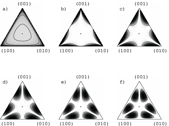
FIG. 2.: Distribution of the eigenvalues of density matrices of size $N=3$ in the simplex of eigenvalues (a) orthogonal product measure, (b) Bures measure, (c) Hilbert-Schmidt measure equal to $P_{3,3}$, other measures induced by partial tracing: (d) $P_{3,4}$, (e) $P_{3,5}$ and (f) $P_{3,6}$.

B Averages over induced measure

Let us now calculate some moments with respect to the Hilbert-Schmidt measure $P_{HS}(\Lambda)=P_{N,N}(\Lambda)$. Taking Fourier representation of the delta function $\delta(1-\sum_{i}\lambda_{i})$ one sees that averages which are homogeneous functions of some ${\lambda}_{k}$ are related to the corresponding moments of the Laguerre ensemble:

$$P_{L}(\lambda_{1},...\lambda_{N})\propto\exp(-\sum_{i}\lambda_{i})\prod_{i}\lambda_{i}^{K-N}\theta(\lambda_{i})\prod_{i<j}(\lambda_{i}-\lambda_{j})^{2}.$$ (33)

Here simple moments can be calculated by the method of orthogonal polynomials [16]. For example one finds for $K=N$ and $\nu>-1$

$$\langle{\rm Tr}{\varrho}^{\nu}\rangle_{HS}\ =\ B_{N,\nu}\int_{0}^{\infty}{\rm d}x\ x^{\nu}\sum_{n=0}^{N-1}L_{n}(x)^{2}{\rm e}^{-x}\ ,$$ (34)

with the Laguerre polynomials defined by

$$L_{n}(x)={\rm e}^{x}\frac{1}{n!}(\frac{d}{dx})^{n}x^{n}{\rm e}^{-x}$$ (35)

and $B_{N,\nu}$ a constant which results from the map of the Hilbert Schmidt measure to the Laguerre measure:

$$B_{N,\nu}=\Gamma(N^{2})/\Gamma(N^{2}+\nu).$$ (36)

Note that we also obtain an explicit expression for the entropy $H(\varrho)=-\langle{\rm Tr}{\varrho}{\rm ln}{\varrho}\rangle$ by taking the derivative of Eq.(34) at $\nu=1$. This can be written as a sum of Digamma functions. For large $N$ it displays asymptotic behaviour

$$\langle H({\varrho})\rangle_{HS}\approx\ln N-\frac{1}{2}+O\bigl{(}\frac{\ln N}{N}\bigr{)}.$$ (37)

This formula gives one of the main results of this paper – the mean entanglement of pure states of the $N\times N$ bipartite system, averaged over the natural measure on the space of pure states. It is equivalent to $\langle H({\varrho})\rangle_{HS}\approx\ln(0.6065N)$, which stays in agreement with recent numerical results of Lakshminarayan [31], who computed mean entanglement of pure states of an exemplary chaotic quantum system – the four dimensional, generalized standard map without time reversal symmetry. Our result is somewhat similar to the asymptotics of the mean entropy of complex random vectors $\langle H(|\phi\rangle)\rangle_{{\mathbb{C}}P^{N-1}}\approx\ln N-1+\gamma$ [7], where the Euler constant $\gamma\sim 0.5772$.

The recurrence relation

$$xL_{n}(x)=-(n+1)L_{n+1}(x)+(1+2n)L_{n}(x)-nL_{n-1}(x)$$ (38)

implies for $\nu=2$

$$\langle{\rm Tr}{\varrho}^{2}\rangle_{HS}=\frac{1}{N^{2}(N^{2}+1)}\sum_{n=0}^{N-1}((n+1)^{2}+(1+2n)^{2}+n^{2})$$ (39)

Finally the sum over $n$ can be done with the result:

$$\langle{\rm Tr}{\varrho}^{2}\rangle_{HS}=\frac{2N}{N^{2}+1}$$ (40)

Using the recurrence relation for the $L_{n}(x)$ one can find the term $\propto L_{n}(x)$ in the Laguerre expansion of $x^{\nu}L_{n}(x)$ for large $n$. From this we find the following asymptotic behavior for large $N$:

$$\langle{\rm Tr}{\varrho}^{\nu}\rangle_{HS}=\frac{\Gamma(1+2\nu)\ N^{1-\nu}}{\Gamma(1+\nu)\Gamma(2+\nu)}\ (1+O(\frac{1}{N})).$$ (41)

This implies for the entropy an asymptotic behavior (37). Inspecting the recurrence relation further one sees that the moments in question are always given by the ratio of two polynomials of $N$. With this knowledge it is easy to calculate some further moments:

$$\langle{\rm Tr}{\varrho}^{3}\rangle_{HS}\ =\ \frac{5N^{2}+1}{(N^{2}+1)(N^{2}+2)}$$ (42)

and

$$\langle{\rm Tr}{\varrho}^{4}\rangle_{HS}\ =\ \frac{14N^{3}+10N}{(N^{2}+1)(N^{2}+2)(N^{2}+3)}.$$ (43)

Finally let us mention that the result for the second moment can be generalised for density matrices distributed according to (30) for arbitrary $N$ and $K$

$${\langle{\rm Tr}{\varrho}^{2}\rangle}_{N,K}\ =\ {\frac{N+K}{NK+1}}\ .$$ (44)

The calculation leads to the generalised Laguerre polynomials. Due to the symmetry in $K$ and $N$ it is even not necessary to mention what is the largest of both dimensions $K$ or $N$. The participation ratio reads thus $R=(NK+1)/(N+K)$ and is consistent with recent results of Zanardi et al. [32]. They computed the linear entropy $1-{\rm tr}\varrho^{2}$ for an ensemble of mixed states obtained by partial tracing of pure states $U(|\psi_{1}\rangle\otimes|\psi_{2}\rangle)$, where $|\psi_{1}\rangle$ and $|\psi_{2}\rangle$ are pure states distributed according to the natural measure on ${\mathbb{C}}P^{N-1}$ (${\mathbb{C}}P^{K-1})$, and $U$ is a random unitary matrix generated according to the Haar measure on $U(NK)$. It is easy to see that this construction leads to the induced measure $P_{N,K}$ given by (30), since the Haar measure on $U(NK)$ is invariant with respect to multiplication by product matrices $U(N)\otimes U(K)$ representing local operations. Thus our results concern not only average entanglement of pure states, but in spirit of [32] also averaged entangling power of global unitary operators.

IV Generalized ensembles of density matrices

One may obtain a different ensemble of density matrices starting from a real pure state with time reversal symmetry

$${{\varrho}}=\sum_{k=1}^{K}u_{ik}{u_{jk}}$$ (45)

with real $u_{ik}$. The only constraint we have now is $\sum_{ik}u_{ik}^{2}=1$. Again we may restrict to $K\geq N$ and since ${\varrho}$ is positive definite we can make the transformation

$$u=\sqrt{{\varrho}}{\tilde{u}},~{}~{}~{}$$ (46)

Now the matrix-delta function of the real symmetric matrix transforms according to

$$\delta(\sqrt{{\varrho}}(1-\tilde{u}\tilde{u}^{\top})\sqrt{{\varrho}})\ =\ {\rm det}{\varrho}^{(-N-1)/2}\ \delta(1-\tilde{u}\tilde{u}^{\top})\ ,$$ (47)

such that

$$P({\varrho})\propto\theta({\varrho})\ \delta({\rm Tr}{\varrho}-1)\ {\rm det}{\varrho}^{(K-N-1)/2}$$ (48)

and the distribution of eigenvalues is given by

$$P^{(1)}(\lambda_{1},\dots,\lambda_{N})\propto\delta(1-\sum_{i}\lambda_{i})\prod_{i}\lambda_{i}^{(K-N-1)/2}\theta(\lambda_{i})\prod_{i<j}|\lambda_{i}-\lambda_{j}|.$$ (49)

Thus $P_{N,K}=P^{(2)}_{N,K}$ corresponds to unitary symmetry with $\beta=2$ and $P^{(1)}$ to orthogonal symmetry with $\beta=1$. Both are special cases of

$$P^{(\beta)}_{N,K}\ =\ C^{(\beta)}_{N,K}\delta(1-\sum_{i}\lambda_{i})\prod_{i}\lambda_{i}^{(\beta(K-N)+\beta-2)/2}\theta(\lambda_{i})\prod_{i<j}|\lambda_{i}-\lambda_{j}|^{\beta}$$ (50)

which can also be given a meaning in the case of symplectic symmetry $\beta=4$ (in that case each Kramers degenerate eigenvalue is counted once and rescaled). In the general case of arbitrary real $\beta>0$ the normalization constant reads

$$C^{(\beta)}_{N,K}=\frac{\Gamma(KN\beta/2)(\Gamma(1+\beta/2))^{N}}{\prod_{j=0}^{N-1}\Gamma((K-j)\beta/2)\Gamma(1+(N-j)\beta/2)}\ .$$ (51)

It can be derived using the map to the Laguerre ensemble and using Selberg’s integral [16]. These ensembles of density matrices may be constructed by generating real ($\beta=1$) or complex ($\beta=2$) random Gaussian matrices $A_{\beta}$ and defining random density matrices by $\varrho=A_{\beta}A_{\beta}^{\dagger}/({\rm tr}A_{\beta}A_{\beta}^{\dagger})$. In the case of symplectic symmetry $(\beta=4)$ one has complex matrices $A_{\beta}$ but then takes only the selfdual part of $\rho$. In fact, any density $P(A)$, in the space of complex density matrices of size $N$ generates in this way a certain ensemble of density matrices of this size.

Let us mention that non-negative matrices $AA^{\dagger}$ are sometimes called random Wishart matrices. The joint probability distribution of their eigenvalues (i.e. the distribution of singular values of $A$) was analyzed in [33, 34]. Real random matrices $A_{1}A_{1}^{T}$ may describe the matrix of correlations between time series of different stock prices in the presence of noise. This fact explains a recent interest in their spectral properties (or in the distribution of singular values of real random matrices $A_{1}$), from the point of view of mathematical finances [35, 36, 37]. Thus the theory of random matrices provides an unexpected link between the computation of the mean entanglement of a certain ensemble of composite quantum states and the estimation of the financial risk [38].

V Concluding remarks

We described various ways of defining ensembles in the space of density matrices of finite size $N$. While it is natural to take eigenvectors distributed according to the Haar measure on $U(N)$, there are several possibilities of introducing the measure into the $(N-1)$ dimensional simplex of eigenvalues. Besides measures related to random vectors (of orthogonal or unitary matrices), one may define measures related to distances in the space of density matrices (say, Hilbert-Schmidt measure or Bures measure).

An alternative way consists in assuming certain measures in more dimensional spaces (e.g. in the space of pure states in $NK$ dimensions or in the $N^{2}$ dimensional space of square matrices of size $N$), and considering the measures induced by projection onto the simplex. We generalized the results of Hall [4] deriving an explicit formula for $P_{N,K}$ and proved that the measure induced by symmetric partial tracing, $P_{N,N}$ coincides with the Hilbert-Schmidt measure (15). We succeeded in computing some averages with respect to this measure including an explicit formula for the Shannon entropy of the reduced density matrix, equal to the mean entropy of entanglement, averaged over the manifold of pure states of the composite $N\times N$ system.

Moreover, we demonstrated a link between the H-S measure determining the spectra of the reduced density matrices and the singular values of the random matrices distributed according to the Ginibre ensemble. As a by–product we demonstrated that $N^{2}$ random complex (real) numbers drawn with respect to the normal distribution, which constitute a non-Hermitian (non-symmetric) random matrix, can be considered as a vector of the unitary (orthogonal) random matrix of size $N^{2}$, drawn according to the Haar measure on $U(N^{2})$ (on $O(N^{2})$). It would be interesting to find an ensemble of random matrices corresponding to Bures measure (18), to compute the normalization constants $C_{N}^{\prime}$ for arbitrary $N$ and to evaluate the mean entanglement averaged with respect to this measure.

It is a pleasure to thank Paweł Horodecki, Marek Kuś and Thomas Wellens for inspiring discussions. Financial support by Komitet Badań Naukowych in Warsaw under the grant 2P03B-072 19, the Sonderforschungsbereich ’Unordnung und große Fluktuationen’ der Deutschen Forschungsgemeinschaft and the European Science Foundation is gratefully acknowledged.

Note added: After this work was completed we learned form M.J.W. Hall about related papers published on this subject: the distribution (30) was derived by Lloyd and Pagels [39], while the formula for the mean entropy averaged over the induced measures was conjectured by Page [40] and proved by Sen [41], (see note added to [4], preprint ArXiv quant-ph/9802052). We are grateful to M.J.W. Hall for helpful correspondence.

A Rescaling of random Gaussian variables

We are going to analyze the joint probability distribution of independent random numbers $y^{\prime}_{i}$, rescaled according to

$$y^{\prime}_{i}\rightarrow y_{i}=\frac{y^{\prime}_{i}}{\sum_{i=1}^{N}y^{\prime}_{i}}\ .$$ (A1)

We assume that each random number is drawn according to the same probability distribution $P(y^{\prime})$ defined for positive $y^{\prime}$. It is easy to see that the joint distribution of the rescaled variables, $P(y_{1},...,y_{N})$, defined in the interval $I=[0,1]$, is symmetric with respect to exchange of any variables, $y_{i}\longleftrightarrow y_{k}$. It is worth to point out that the uniform initial distribution, $P(y^{\prime}_{i})=1$ for $y^{\prime}\in[0,1]$ does not produce the uniform distribution of the rescaled variables, but $P(y_{1}....y_{N})=\delta(1-\sum_{i}y_{i})/(N({\rm max}\{y_{i}\})^{N})$. In the simplest case, $N=2$, it gives $P(y)=1/(2(1-y)^{2})$ for $y<1/2$, (where $y=y_{1}=1-y_{2}$) and symmetrically for $y>1/2$.

Let us now assume that the random numbers are given by squares of Gaussian random numbers, $y_{i}^{\prime}=x_{i}^{2}$ and $P(x_{1},x_{2},...x_{N})\propto\exp(-\sum_{i}x_{i}^{2})$. We want to calculate the distribution of the rescaled variables $y_{i}=x_{i}^{2}/\sum_{i}x_{i}^{2}$:

$$P(y_{1},y_{2},...y_{N})\propto\int{\rm d}x_{1}...{\rm d}x_{N}\exp(-\sum_{i}x_{i}^{2})\prod_{i}\delta(y_{i}-x_{i}^{2}/\sum_{i}x_{i}^{2})\ .$$ (A2)

Introducing a $\delta$ function for the constraint $t=\sum_{i}x_{i}^{2}$ we have

$$P(y_{1},y_{2},...y_{N})\propto\int_{0}^{\infty}{\rm d}t{\rm e}^{-t}\int{\rm d}x_{1}...{\rm d}x_{N}\delta(t-\sum_{i}x_{i}^{2})\prod_{i}\delta(y_{i}-x_{i}^{2}/t)$$ (A3)

If we now rescale $x_{i}\to x_{i}\sqrt{t}$ we obtain

$$P(y_{1},y_{2},...y_{N})\propto\int_{0}^{\infty}{\rm d}t{\rm e}^{-t}t^{-1+N/2}\int{\rm d}x_{1}...{\rm d}x_{N}\delta(1-\sum_{i}x_{i}^{2})\prod_{i}\delta(y_{i}-x_{i}^{2})$$ (A4)

which yields the Dirichlet distribution (12) with $s=1/2$.

This result may be generalized for the sum of $\beta$ squared random numbers drawn according to the normal distribution, $y_{i}^{\prime}=\sum_{j=1}^{\beta}x_{i,j}^{2}$, the distribution of the sum is given by the $\chi^{2}_{\beta}$ distribution with $\beta$ degrees of freedom. In an analogous way we obtain that the joint distribution of $y_{i}$’s rescaled as in (A1) is given by the Dirichlet distribution

$$P(y_{1},y_{2},...,y_{N})\propto\delta(1-\sum_{i}y_{i})\prod_{i=1}^{N}y_{i}^{\beta/2-1},$$ (A5)

with $s=\beta/2$. The most important case, $\beta=2$, shows that the distribution of squared components of a rescaled complex vector of Gaussian random numbers is uniform in the $(N-1)$ dimensional simplex.

Above results find following simple applications. Real (complex) random vectors, i.e. columns (or rows) of orthogonal (unitary) random matrix may be constructed out of independent random Gaussian numbers (real or complex, respectively) rescaled according to Eq. (A1). This is consistent with the well known fact that the distribution of squared components of eigenvectors of a GOE (GUE) matrix are given by the $\chi_{\beta}^{2}$ distribution with $\beta=1$ (or $2$) degrees of freedom [16]. Thus certain averages, one wants to compute averaging over the set of pure states (say, entropy, participation ratio, etc), may be replaced by averages over the simplex in $R^{N-1}$ with the Dirichlet measure (12) with $s=1/2$ or $s=1$.

Furthermore, a complex square random matrix $\psi_{kl}^{\prime}$ of size $N$ pertaining to the Ginibre ensemble after rescaling $\psi^{\prime}\rightarrow\psi=\psi^{\prime}/\sqrt{{\rm tr}{\psi^{\prime}}^{\dagger}\psi^{\prime}}$ represents a random pure state drawn according to the natural measure on ${\mathbb{C}}P^{N^{2}-1}$. A similar link is established between rescaled rectangular matrices of size $K\times N$ and the elements of ${\mathbb{C}}P^{KN-1}$. Analogously, normalized non-symmetric real random matrices with each element drawn independently according to the normal distribution are equivalent to random vectors distributed with respect to the natural measure on the real projective space, ${\mathbb{R}}P^{N^{2}-1}$.

REFERENCES

- [1] Życzkowski K, Horodecki P, Sanpera A and Lewenstein M 1998 Phys. Rev. A 58, 833
- [2] Slater P B 1999 J. Phys. A 32, 5261
- [3] Życzkowski K 1999 Phys. Rev. A 60, 3496
- [4] Hall M J W 1998 Phys. Lett. A 242, 123
- [5] Slater P B 1998 Phys. Lett. A 247, 1
- [6] Wootters W K 1990 Found. Phys. 20, 1365
- [7] Jones K R W 1990 J. Phys. A 23, L1247
- [8] Jones K R W 1991 Ann. Phys. (N.Y.) 207, 140
- [9] Braunstein S L 1996 Phys. Lett. A 219 169
- [10] Bengtsson I 1998 Lecture notes on Geometry of Quantum Mechanics, unpublished
- [11] Horn R and Johnson C 1991 Topics in Matrix Analysis, Cambridge University Press
- [12] Hurwitz A 1897 Nachr. Ges. Wiss. Gött. Math.-Phys. Kl. 71
- [13] Poźniak M, Życzkowski K and Kuś M 1998 J. Phys. A 31, 1059
- [14] Barros e Sá N 2001 J. Math. Phys. 42, 981
- [15] Adelman M, Corbett J V and Hurst C A 1993 Found. Phys. 23, 211
- [16] Mehta M L 1991 Random Matrices, II ed. Academic, New York,
- [17] Haake F 1991 Quantum Signatures of Chaos (Springer: Berlin)
- [18] Slater P B 1999 J. Phys. A 32, 8231
- [19] Fisher R A 1930 Proc. Roy. Soc. Edin. 50, 205
- [20] Mahalonobis P C 1936 Proc. Nat. Inst. Sci. India 12, 49
- [21] Frieden B R 1991 Probability, Statistical Optics and Data Testing Berlin, Springer-Verlag
- [22] Petz D and Sudár C 1996 J. Math. Phys. 37, 2662
- [23] Życzkowski K and Słomczyński W 2000 LANL preprint quant-ph/0008016
- [24] Bures D J C 1969 Trans. Am. Math. Soc. 135, 199
- [25] Uhlmann A 1976 Rep. Math. Phys. 9, 273
- [26] Uhlmann A 1992 in Groups and related Topics, P. Gierelak et. al. (eds.), Kluver, Dodrecht
- [27] Hübner M 1992 Phys. Lett. A 163, 239
- [28] Byrd M S and Slater P B 2000 LANL preprint quant-ph/0004055
- [29] Wootters W K 1998 Phys. Rev. Lett. 80, 2245
- [30] Kendon V M, Nemoto K and Munro W J 2001 LANL preprint quant-ph/0106023
- [31] Lakshminarayan A 2000 LANL preprint quant-ph/0012010
- [32] Zanardi P, Zalka C and Faoro L 2000 Phys. Rev. A 62, 30301
- [33] Baker T H, Forrester P J and Pearce P A 1998 J. Phys. A 31, 6087
- [34] Sengupta A M and Mitra P P 1999 Phys. Rev. E 60, 3389
- [35] Laloux L, Cizeau P, Bouchaud J P, Potters M 1999 Phys. Rev. Lett. 83, 1467
- [36] Plerou V, Gopikrishnan P, Rosenow B, Amaral L A N and Stanley H E 1999 Phys. Rev. Lett. 83, 1471
- [37] Nowak M and Jurkiewicz J 2001 to be published
- [38] Bouchaud J P and Potters M 1997 Theory of Financial Risk (in French), Eyrolles, Paris
- [39] Lloyd S and Pagels H 1988 Ann. Phys. (N.Y.) 188, 186
- [40] Page D 1993 Phys. Rev. Lett. 71, 1291
- [41] Sen S 1996 Phys. Rev. Lett. 77, 1