Time evolution and squeezing of the field amplitude in cavity QED

Abstract

We present the conditional time evolution of the electromagnetic field produced by a cavity QED system in the strongly coupled regime. We obtain the conditional evolution through a wave-particle correlation function that measures the time evolution of the field after the detection of a photon. A connection exists between this correlation function and the spectrum of squeezing which permits the study of squeezed states in the time domain. We calculate the spectrum of squeezing from the master equation for the reduced density matrix using both the quantum regression theorem and quantum trajectories. Our calculations not only show that spontaneous emission degrades the squeezing signal, but they also point to the dynamical processes that cause this degradation.

OCIS codes:(270.0270) Quantum Optics; (270.6570) Squeezed States; (270.2500) Fluctuations, relaxations, and noise.

I Introduction

Squeezing experiments focus on the control and study of quantum fluctuations. In a squeezed state there is a redistribution of the fluctuations between the different quadratures of the electromagnetic field. The modification is measurable through the spectrum of squeezing and its comparison with that of the vacuum state. In this paper we analyze the time evolution of the quantum fluctuations of the electromagnetic field, the complementary picture of the spectral density studied in squeezing. We use a new formalism based on a third order correlation function of the field. This wave-particle correlation combines conditional measurements with the process of quantum measurement. The quantum fluctuations are related to the measurement process and, in a strongly coupled system, those fluctuations can be orders of magnitude larger than the steady state.

By combining the wave and particle aspects of light, this correlation function brings a new theoretical [1] and experimental [2, 3] understanding to the study of the quantum properties of squeezed light. This is because the wave-particle correlation function and the spectrum of squeezing form a Fourier transform pair when third order moments of the field fluctuations are neglected. We can now analyze the conditional time evolution of the fluctuations that give rise to the redistribution of the noise between the two quadratures of the electromagnetic field.

Work on the spectrum of squeezing is a well established area of research [4, 5]. The interaction between a single cavity mode of the electromagnetic field and several two level atoms produce non-classical fields which exhibit squeezing. Work on this system started with the problem of optical bistability (OB) [6, 7, 8, 9, 10]. These OB systems are treated in the limit of small noise, such that the fluctuations are only a minimal perturbation on the steady state. More recent work has focused on a regime where there is no small size parameter and fluctuations dominate the behavior of the system [11]. This general area is cavity QED [12]. While there are experimental realizations in the microwave and optical regimes, our discussion will only consider the latter. In both systems the reversible coupling between the atoms and the cavity mode is larger than the irreversible loss of coherence from spontaneous emission or cavity decay. A number of optical studies, experimental and theoretical, have focused on the non-classical features as observed in the intensity correlations, eg. photon antibunching [13, 14, 15, 16]. Our recent observations look, however, at the time dependence of the conditional fluctuations of the field [2] and its connection with the spectrum of squeezing.

We found from experiment that the spectrum of squeezing was degraded when the conditional fluctuation oscillated around a value different from the steady state field amplitude. In order to understand this behaviour we apply the time domain formalism to the strong coupling regime of cavity QED. To keep the discussion manageable we only treat the case of one or two atoms fixed in space. The work follows the general philosophy established in Refs. [17, 18] where cavity QED is analyzed without a small parameter.

The paper is organized as follows. In section II, we describe the wave-particle correlation function and its connection to the spectrum of squeezing. Section III discusses the properties of the cavity QED system. Section IV shows the different techniques utilized to calculate the spectrum of squeezing and the wave-particle correlation function. We present our results in section V, the discussion of those results in section VI, and our conclusions in section VII.

II The wave-particle correlation function

Figure 1 shows the apparatus that measures the correlation between the amplitude and the intensity of the electromagnetic field. The particle (photon) produces a trigger ‘click’ in an avalanche photo diode (APD) and conditionally the wave (electromagnetic field amplitude) gets recorded in the photocurrent output of a balanced homodyne detector (BHD). The observations of Ref. [2] consider a conditioned field evolution described by a third order correlation function of an electromagnetic field mode $\hat{b}$ (signal) that has a non-zero, steady state average $\langle\hat{b}\rangle=\lambda$. The measured correlation is

$$h_{\theta}(\tau)=\frac{\langle:\!(\hat{b}^{\dagger}\hat{b})(0)\hat{Q}_{\theta}(\tau)\!:\rangle}{\sqrt{\eta}\lambda\langle\hat{b}^{\dagger}\hat{b}\rangle},$$ (1)

where $\hat{Q}_{\theta}\equiv(\hat{b}{\rm{exp}}(-i\theta)+\hat{b}^{\dagger}{\rm{exp}}(i\theta))/2$ is the quadrature amplitude selected by the local oscillator phase $\theta$ and $\eta$ is the coupling efficiency into the BHD. Carmichael et al. have generalized Eq. (1) to any source [1], but for the purpose of this paper it is sufficient to limit the discussion to the detection scheme of Fig. 1.

We separate the fluctuations from the mean field writing,

$$\hat{b}=\lambda{\rm{exp}}(i\theta)+\Delta\hat{b}$$ (2)

The correlation function can be rewritten in terms of the field fluctuations. In the limit of Gaussian fluctuations we may neglect third-order moments of the field fluctuations and the correlation function is [2]

$$h_{0^{\circ}}(\tau)=1+2\frac{\langle:\!\Delta\hat{Q}_{0^{\circ}}(0)\Delta\hat{Q}_{0^{\circ}}(\tau)\!:\rangle}{\lambda^{2}+\langle\Delta\hat{b}^{\dagger}\Delta\hat{b}\rangle}+\xi(\tau),$$ (3)

where $\Delta\hat{Q}_{0^{\circ}}\equiv(\Delta\hat{b}+\Delta\hat{b}^{\dagger})/2$ and $\xi(\tau)$ is the residual shot noise with the following correlation function

$$\overline{\xi(0)\xi(\tau)}=\frac{\Gamma}{16\eta N_{s}|\langle\hat{b}\rangle|^{2}}{\rm{exp}}(-\Gamma\tau)$$ (4)

where $\Gamma$ is the BHD bandwidth. It is apparent from Eq. (4) that once the conditioned field is normalized for a fixed $|\langle\hat{b}\rangle|^{2}$ then the shot noise, $\xi(t)$, is determined by the detection bandwidth and the number of samples averaged. Therefore one must average over many start “clicks” to obtain a good signal to noise ratio.

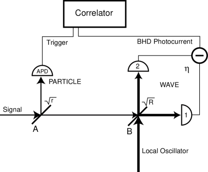
FIG. 1.: Schematic of the wave particle correlator.

The spectrum of squeezing is the cosine transform of the normalized correlation function,

$$S(\theta,\nu)=4F\int_{0}^{\infty}d\tau\cos(2\pi\nu\tau)[\overline{h_{\theta}(\tau)}-1],$$ (5)

where $F=2\kappa\langle\hat{b}^{\dagger}\hat{b}\rangle$ is the photon flux into the correlator and $\overline{h_{\theta}(\tau)}$ is the average of $h_{\theta}(\tau)$ with respect to $\xi(\tau)$. This average is independent of the fraction of light, $1-r$, sent to the BHD.

The wave-particle correlator has two practical advantages over a standard squeezing measurement. First, the fluctuations in time reveal the entire spectrum of squeezing up to a frequency set by the detector bandwidth. The second is that the BHD efficiency only enters through the residual shot noise in Eq. (3). This shot noise can be made to vanish by averaging over many trigger starts. This implies that the spectrum of squeezing is not degraded by imperfect detector efficiencies and propagation errors which beset the standard squeezing measurement.

III Cavity QED system

The fluctuations in the signal beam in Fig. 1 must be squeezed by a non-linear source. The source we consider here originates from a cavity QED system. The cavity QED system consists of a single mode of the electromagnetic field interacting with a collection of two-level atoms (see Fig. 2). Two spherical mirrors that form a standing-wave optical cavity define the field mode. We consider only a single or a pair of two level atoms optimally coupled to the mode of the cavity. Dissipation plays an important role as both the atoms and the field couple to reservoirs. An atom can spontaneously emit light into modes other than the preferred mode, and light inside the cavity can escape through the mirrors. We assume that the fractional solid angle subtended by the cavity mode is small enough so that we do not have to make corrections to the atomic decay rates. A coherent field, injected through one of the mirrors, drives the system. The signal beam in Fig. 1 is the light that escapes from the cavity through the output mirror.

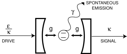
FIG. 2.: Schematic of the cavity QED system.

The Jaynes-Cummings Hamiltonian [19] describes the interaction of a two-level atom with a single mode of the quantized electromagnetic field.

$$\hat{H}=\hbar\omega_{\rm a}\hat{\sigma}^{z}+\hbar\omega_{\rm c}\hat{a}^{\dagger}\hat{a}-i\hbar g(\hat{\sigma}_{+}\hat{a}-\hat{a}^{\dagger}\hat{\sigma}_{-})$$ (6)

where $\hat{\sigma}_{\pm}$ and $\hat{\sigma}^{z}$ are the Pauli spin operators for raising, lowering, and inversion of the atom, and $\hat{a}^{\dagger},\hat{a}$ are the raising and lowering operators for the field. The eigenstates for Eq. (6) reveal the entanglement between the atom and the field. The spectrum has a first excited state doublet with states shifted by $\pm g$ from the uncoupled resonance. The dipole coupling constant, $g$, is given by:

$$g=\left(\frac{\mu^{2}\omega}{2\hbar\epsilon_{0}V}\right)^{1/2}$$ (7)

where $\mu$ is the transition dipole moment, $\omega$ is the transition frequency, and V is the cavity mode volume. The field decays out of the cavity at the rate of $\kappa$ and, considering only radiative decay, the atomic inversion decays at the rate of $\gamma=1/\tau$ ($\tau$ is the radiative lifetime of the atomic transition).

From $g$, $\gamma$ and $\kappa$ we can construct two dimensionless numbers from the OB literature that are useful for characterizing cavity QED systems: the saturation photon number $n_{0}$ and the single atom cooperativity $C_{1}$. They scale the influence of a photon and the influence of an atom in the system. These two numbers relate the reversible dipole coupling between a single atom and the cavity mode ($g$) with the irreversible coupling to the reservoirs through cavity ($\kappa$) and inversion decays ($\gamma$) by

$$C_{1}=g^{2}/\kappa\gamma$$ (8)

and for a plane wave cavity field with the atoms sitting at the anti-nodes,

$$n_{0}=\gamma^{2}/8g^{2}.$$ (9)

They define the different regimes of OB and cavity QED. The strong coupling regime of cavity QED, $n_{0}<1$ and $C_{1}>1$, implies large effects from the presence of a single photon and of a single atom in the system. Consequently, a change of one photon is a large fluctuation in the system.

We only consider the resonant case here, with the driving field on resonance with the atomic transition and cavity mode frequencies. This means that we are only able to explore dynamical changes in one quadrature. In order to generalize to other phases one must either drive the system off resonance or add a coherent offset like the one discussed in Ref. [1].

Two dimensionless fields and intensities follow from the OB literature that allow us to make contact with experiments: The intracavity field (intensity) with atoms in the cavity $x\equiv\langle\hat{a}\rangle/\sqrt{n_{0}}$; ($X\equiv\langle\hat{a}^{\dagger}\hat{a}\rangle/n_{0}$), and the field (intensity) without atoms in the cavity $y\equiv{\mathcal{E}}/\kappa\sqrt{n_{0}}$; ($Y=y^{2}$) where $2{\mathcal{E}}^{2}/\kappa$ is the input photon flux.

IV Calculations of the wave-particle correlation function in cavity QED

We present the two different methods used to calculate the wave-particle correlation function. The first is a direct calculation from the master equation and the second is a quantum trajectory simulation.

A Direct Calculation from the Master Equation

A master equation of the Lindblad form can be derived for the system shown in Fig. 2 using standard techniques (see for example [20]). This equation for the reduced density operator $\hat{\rho}$ for the case of $N$-atoms identically coupled to a single cavity mode reads

$$\dot{\hat{\rho}}\equiv{\mathcal{L}}{\hat{\rho}}={\mathcal{E}}[\hat{a}^{\dagger}-\hat{a},\hat{\rho}]+g[\hat{a}^{\dagger}\hat{S}_{-}-\hat{a}\hat{S}_{+},\hat{\rho}]$$ (12)

$$\mbox{}+\kappa(2\hat{a}\hat{\rho}\hat{a}^{\dagger}-\hat{a}^{\dagger}\hat{a}\hat{\rho}-\hat{\rho}\hat{a}^{\dagger}\hat{a})$$

$$\mbox{}+\gamma/2\sum_{j=1}^{N}(2\hat{\sigma}^{j}_{-}\hat{\rho}\hat{\sigma}^{j}_{+}-\hat{\sigma}^{j}_{+}\hat{\sigma}^{j}_{-}\hat{\rho}-\hat{\rho}\hat{\sigma}^{j}_{+}\hat{\sigma}^{j}_{-}),$$

where $\hat{S}_{\pm}=\sum_{j}\sigma^{j}_{\pm}$ are the collective raising and lowering operators for the atoms.

Early attempts to solve this master equation are found in the OB literature [6, 7]. They involved converting the master equation into a $c$-number Fokker-Planck equation via a large $N$ expansion. A connection was then made to a set of Itô stochastic differential equations. This master equation could thus be solved analytically, but only for the case of small fluctuations.

Our cavity QED system operates in the strongly coupled regime where the effective number of atoms and the size of the quantum fluctuations, relative to the steady state, will not permit us to make any of the assumptions mentioned above. Instead we numerically solve the master equation in a manner similar to that described by Brecha et al [18]. We transform the master equation into frequency space and apply the quantum regression theorem of Lax [21] to calculate the spectrum of squeezing directly. We check the accuracy of our results by increasing the maximum number of photons included in the basis, $n_{\rm max}$, until the value of the squeezing at any given frequency is accurate to three significant digits. This approach permits us to calculate the spectrum of squeezing for the cavity QED system away from the low intensity limit and it allows us to consider the case of either one or two atoms.

B Quantum Trajectories

Studying quantum trajectories with the wave-particle correlator requires some justification. This section provides that justification. We begin with a review of some of the fundamental concepts behind quantum trajectory theory. Much of the important work done in the field of quantum trajectories and stochastic Schrodinger equations can be found in the review article by Plenio and Knight [22] and references therein. This presentation follows the work of Carmichael [20].

An alternative approach to studying a master equation of the Lindblad form can be formulated with quantum trajectory theory. To create quantum trajectories one must unravel the master equation. We are only interested in those unravellings which correspond directly to an experimental measurement. This measurement probes the system by opening channels between the system and the environment. Excitations into these channels are represented by the following superoperator

$${\mathcal{S}}_{i}\hat{\rho}=\hat{k}(\hat{s_{i}},\hat{s_{i}}^{{\dagger}})\hat{\rho}\hat{k}^{{\dagger}}(\hat{s_{i}},\hat{s_{i}}^{{\dagger}})$$ (13)

where ${\hat{k}}$ is a function of the creation and annihilation operators, ${\hat{s}_{i}^{{\dagger}}}$ and ${\hat{s}_{i}}$, for the $i^{th}$ system operator coupled to the environment. The probability for the system to decay through one of these channels depends on the occupation of that particular mode,

$$P_{i}=\rm{Tr}({\mathcal{S}}_{\it i}\hat{\rho})\it{dt}$$ (14)

Quantum trajectories also provide a picture of what is happening to the system between measurements. Equation (13) describes how measurements are performed on the system. To see what happens between measurements, subtract Eq. (13) from Eq. (12),

$$({\mathcal{L}}-{\sum_{i}{\mathcal{S}}_{i}})\hat{\rho}=\frac{1}{i\hbar}(\hat{H}_{\rm sys}\hat{\rho}-\hat{\rho}\hat{H}_{\rm sys}^{\dagger})$$ (15)

If we assume that the system state is initially pure then Eqs. (13) and (15) guarantee that the conditional density operator can be written in the factorized form $\rho=|\psi\rangle\langle\psi|$. Therefore Eq. (15) implies that a propagator exists for the system wavefunction between measurements. This propagator is a modified, non-unitary, Hamiltonian with a real and imaginary part, $\hat{H}_{\rm sys}=\hat{H}_{R}+i\hat{H}_{I}$.

Below is the quantum trajectory algorithm which propagates the system wavefunction forward in time.

1. Choose an initial state for the system.

2. Calculate the probability for the system to decay through each of the loss channels from Eq. (14).

$$P_{i}=\langle\hat{k}^{\dagger}(\hat{s}_{i})\hat{k}(\hat{s}_{i})\rangle dt$$ (16)

3. Associate a uniformly distributed random number between 0 and 1 with each loss channel in step 2. If the probability for the $i^{th}$ channel is greater than its corresponding random number then collapse the system wavefunction,

$$|\psi(t+dt)\rangle=\hat{k}(\hat{s}_{i})|\psi(t)\rangle$$ (17)

In the unlikely event of multiple collapses, choose only one collapse via another random number.

4. If the probability for loss through each channel is less than the corresponding random numbers, then propagate the system wavefunction with the effective Hamiltonian from Eq. (15),

$$|\psi(t+dt)\rangle=(1-\frac{\hat{H}_{\rm sys}}{i\hbar}dt)|\psi(t)\rangle$$ (18)

5. Normalize the system wavefunction and repeat from step 2.

This is the basis for quantum trajectories. The master equation describes the evolution of the reduced density matrix. A connection is made between this density matrix and a system wavefunction. This wavefunction leads to measurements via losses through the system’s decay channels. These measurements update our knowledge of the system wavefunction. This allows one to study how measurements performed on a system will, through conditioning, affect the system state.

In order to unravel Eq. (12) with the wave-particle correlator we need to first add the BHD to the system. The BHD consists of a local oscillator which is modeled by a driven, single mode coherent field. We write the master equation for the system plus local oscillator mode as

$$\dot{\hat{\rho}}={\mathcal{E}}[\hat{a}^{\dagger}-\hat{a},\hat{\rho}]+g[\hat{a}^{\dagger}\hat{S}_{-}-\hat{a}\hat{S}_{+},\hat{\rho}]$$ (22)

$$\mbox{}+\kappa(2\hat{a}\hat{\rho}\hat{a}^{\dagger}-\hat{a}^{\dagger}\hat{a}\hat{\rho}-\hat{\rho}\hat{a}^{\dagger}\hat{a})$$

$$\mbox{}+\kappa_{LO}(2\hat{c}\hat{\rho}\hat{c}^{\dagger}-\hat{c}^{\dagger}\hat{c}\hat{\rho}-\hat{\rho}\hat{c}^{\dagger}\hat{c})+\kappa_{LO}\chi[\hat{c}^{\dagger}-\hat{c},\hat{\rho}]$$

$$\mbox{}+\gamma/2\sum_{j=1}^{N}(2\hat{\sigma}^{j}_{-}\hat{\rho}\hat{\sigma}^{j}_{+}-\hat{\sigma}^{j}_{+}\hat{\sigma}^{j}_{-}\hat{\rho}-\hat{\rho}\hat{\sigma}^{j}_{+}\hat{\sigma}^{j}_{-}),$$

where $\hat{c}^{\dagger}$ and $\hat{c}$ represent the raising and lowering operators for the local oscillator mode. The coherent field occupies a mode whose strength we denote by $\chi$. Under a BHD scheme the beam splitter combines the signal and local oscillator fields equally $(R=1/2)$, as in Fig. 1, to give the following total measured fields at photodetectors 1 and 2

$$\hat{\mathcal{E}}_{\rm BHD^{1,2}}=\pm i\sqrt{\kappa_{\rm LO}}\hat{c}+\sqrt{\kappa(1-r)}\hat{a}$$ (23)

while the measured field at the photon counting detector gives

$$\hat{\mathcal{E}}_{\rm count}=\sqrt{2\kappa r}\hat{a}.$$ (24)

We assume that the signal mode does not affect the local oscillator mode. This implies that the density matrix separates into a piece which corresponds to the cavity QED system and a piece which corresponds to the local oscillator,

$$\hat{\rho}=\hat{\rho}_{s}|\chi\rangle\langle\chi|.$$ (25)

We define the local oscillator flux in terms of the strength of the local oscillator mode and its cavity decay rate.

$$f=\kappa_{\rm LO}|\chi|^{2}.$$ (26)

From Eq. (13) we construct the master equation terms which correspond to Eqs. (23-24) and spontaneous emissions.

$${\mathcal{S}}_{\rm BHD^{1,2}}\hat{\rho}_{s} = (\pm\sqrt{f}e^{i\theta}+\sqrt{2\kappa(1-r)}\hat{a})$$ (28)

$$\times\hat{\rho}_{s}(\pm\sqrt{f}e^{-i\theta}+\sqrt{2\kappa(1-r)}\hat{a}^{\dagger})$$

$${\mathcal{S}}_{\rm count}\hat{\rho}_{s}=2\kappa r\hat{a}\hat{\rho}_{s}\hat{a}^{\dagger}$$ (29)

$${\mathcal{S}}_{\rm spont}\hat{\rho}_{s}=\gamma\hat{\sigma}_{-}\hat{\rho}_{s}\hat{\sigma}_{+}$$ (30)

After subtracting Eqs. (28-30) from Eq. (22), we arrive at an expression which corresponds to Eq. (15).

$$({\mathcal{L}} - {\mathcal{S}}_{\rm BHD^{1,2}}-{\mathcal{S}}_{\rm count}-{\mathcal{S}_{\rm spont}})\hat{\rho}_{s}={\mathcal{E}}[\hat{a}^{\dagger}-\hat{a},\hat{\rho}_{s}]$$ (33)

$$+g[\hat{a}^{\dagger}\hat{S}_{-}-\hat{a}\hat{S}_{+},\hat{\rho}_{s}]-\kappa(\hat{a}^{\dagger}\hat{a}\hat{\rho}_{s}+\hat{\rho}_{s}\hat{a}^{\dagger}\hat{a})$$

$$-\gamma/2\sum_{j=1}^{N}(\hat{\sigma}^{j}_{+}\hat{\sigma}^{j}_{-}\hat{\rho}_{s}+\hat{\rho}_{s}\hat{\sigma}^{j}_{+}\hat{\sigma}^{j}_{-})-f\hat{\rho}_{s}$$

Equation (33) provides a modified Hamiltonian which propagates the system’s wavefunction between measurements. Equations (28) and (29) govern how “clicks” at the BHD and APD disrupt that evolution.

There are two types of detections, not including spontaneous emissions, which occur under the conditional BHD measurement. The first comes from Eq. (29) which corresponds to detections at the APD. According to Eq. (14) these collapses occur with a probability of $2\kappa r\langle\hat{a}^{\dagger}\hat{a}\rangle dt$ and they produce a signifigant change in the wavefunction as is evident from Eq. (17).

The second type of collapse corresponds to the “clicks” at the BHD. The strength of the local oscillator tells us that there are many BHD “clicks” within a time interval set by $\kappa^{-1}$. Eq. (17) shows that the effect of each of these “clicks” on the system wave function is almost negligible. This implies that a straight forward trajectory simulation with the algorithm described above in Eqs. (16-18) will not provide an efficient method for modeling the wave-particle correlator. Instead we may associate a photocurrent with the detections registered by the BHD. The superposition of the cavity field with the local oscillator field in Eq. (23) implies that the BHD photocurrent and the system wavefunction evolution are not independent. With the principles outlined in Sects. 8.4, 9.2, and 9.4 of [20] we combine Eqs. (28-33) to simultaneously calculate this photocurrent from the BHD setup and then evolve a corresponding stochastic Schrödinger equation forward in time. This analysis leads to the following expressions for the difference in photocurrents between photodetectors 1 and 2 in Fig. 1, and wavefunction propagation between photodetections at the APD and spontaneous emissions out the sides of the cavity.

$$di=-\Gamma(idt-\sqrt{8\kappa(1-r)}\langle\hat{a}_{\theta}\rangle_{c}dt+dW_{t})$$ (34)

$$d|\bar{\psi}\rangle_{c}=[\frac{H_{\rm sys}}{i\hbar} d t+\sqrt{2\kappa(1-r)}\hat{a}{\rm{exp}}(-i\theta)$$ (36)

$$\times(\sqrt{8\kappa(1-r)}\langle\hat{a}_{\theta}\rangle_{c}dt+dW_{t})|\bar{\psi}\rangle_{c}$$

where $\Gamma$ is the BHD bandwidth and $dW_{t}$ is the same Wiener noise increment in both equations.

This BHD difference current, $i(t)$, along with a set of start times $\{t_{j}\}$, form a stochastic measurement record. The source quasimode $\hat{a}$ is in a quantum state $|\psi_{\rm REC}(t)\rangle$ conditioned on the past record. We simulate Eqs. (34-36) on a computer. By sampling an ongoing realization of $i(t)$ for many “start” times (APD detections realized concurrently) we may calculate the following averaged photocurrent,

$${\mathcal{H}(\tau)}=\frac{1}{N_{s}}\sum_{j=1}^{N_{s}}i(t_{j}+\tau).$$ (37)

A connection exists between the averaged photocurrent and the wave-particle correlation function [1]. In the limit of large bandwidth this connection reads

$$h_{\theta}(\tau)=\frac{\mathcal{H}(\tau)}{\langle\hat{a}\rangle\sqrt{8\kappa(1-r)}}.$$ (38)

The dual nature of the measurement process provides one of the many strengths of the conditional field measurement. It allows the use of quantum trajectory theory to unravel the master equation in two distinct ways. A numerical simulation of Eqs. (34-36) reproduces the experimental results for the averaged photocurrent. We can understand some of the mechanisms which lead to this averaged result by simulating the algorithm described in Eqs. (16-18) and replacing Eq. (18) with Eq. (36). Setting $r\approx 1$ reduces the conditional homodyne simulation to a cleaner photocounting simulation. This leads to an understanding of the dynamical processes which create the spectrum of squeezing.

V results

The simplest parameter to change during the course of the experiment is the strength of the driving field. This motivates our study of the effect of driving intensity on the spectrum of squeezing. The strength of the driving field is parameterized in terms of the saturation photon number, $n_{\rm{o}}$. Therefore weak fields imply $X\ll 1$, for intermediate fields $X\approx 1$, and strong fields correspond to $X\gg 1$. We begin by reporting the results of a low intensity calculation with both the quantum trajectories and the direct calculation from the master equation. We then increase the intensity of the driving field and also the number of atoms in the cavity from one to two. This degrades the spectrum of squeezing in a way which we hope to understand through the study of quantum trajectories.

A Low Intensity Results for $h(0^{\circ},\tau)$ and $S(0^{\circ},\nu)$

Figure 3 shows the equivalence of the third order correlation function $h(0^{\circ},\tau)$ (i) and the spectrum of squeezing (ii) for a strongly coupled cavity QED system. The dashed line in Fig. 3ii is the spectrum of squeezing calculated directly from the quantum regression theorem. The solid line is the Fourier transform (see Eq. (5)) of Fig. 3i which comes from averaging the photocurrent from a quantum trajectory simulation over 55000 “starts” . Both approaches show the damped Rabi oscillations which follow and precede a photodetction. In the weak field excitation limit, Rice and Carmichael [23] derived an analytical expression for the spectrum of squeezing which agrees with these results.

Detecting a photon in the APD collapses the state of the cavity field. The oscillations in the field after a detection show the collapsed state oscillating back towards the steady state. In the Gaussian noise approximation the time symmetry of the measured correlation function, Eq. (3), guarantees the oscillation before the detection.

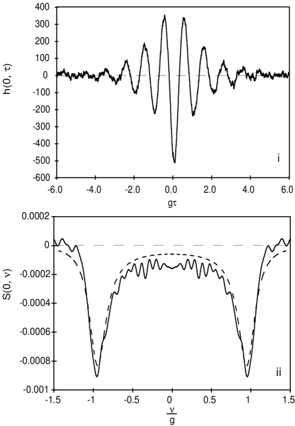
FIG. 3.: i. Wave-particle correlation $h(0^{\circ},\tau)$ for very low intensity excitation calculated from the quantum trajectory implementation of the conditioned homodyne photocurrent. The following parameters were used: $(g,\kappa,\gamma,\Gamma)$/$(2/\pi)$ = $(38.0,8.7,3.0,100)$ MHz, $X=2.99\times 10^{-4}$, $r=0.5$ and $N_{\rm starts}$ = $55000$. ii. Spectrum of squeezing calculated from the cosine Fourier transform of $h(0^{\circ},\tau)$. The dashed line is the spectrum of squeezing calculated directly from the master equation with the quantum regression theorem.

B From one atom to two atoms at intermediate intensity

It has not been possible to obtain analytical expressions for the spectrum of squeezing in the case of intermediate driving fields. In this regime one cannot linearize the system fluctuations about the steady state field as was done in the strong field case [24]. It is also impossible to perform a small parameter expansion in the driving field as was done in the weak field case [17]. We are instead forced to rely on numerical calculations to give us insight into a system’s spectrum of squeezing. This approach has its limitations.

The spectra of squeezing for increased excitation in the case of one and two atoms have distinct quantitative differences. Fig. 4 shows one such spectrum calculated for a driving field of ${\mathcal{E}}$/$\kappa=1.50$ and one atom. Fig. 5 shows the result for two atoms with ${\mathcal{E}}$/$\kappa=0.975$. We calculated both plots with the same decay parameters but different atom field couplings, $g$ to keep the Rabi frequency, $g\sqrt{N}$, the same.

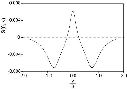
FIG. 4.: The spectrum of squeezing calculated directly from the master equation with the quantum regression theorem for N=1 and high intensity. $X=104.0$, $(g,\kappa,\gamma)$/$(2\pi)$ = $(38.0,8.7,3.0)$ MHz.

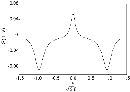
FIG. 5.: The spectrum of squeezing calculated directly from the master equation with the quantum regression theorem for N=2 and intermediate intensity. $X=1.36$, $(g,\kappa,\gamma)/(2\pi)$ = $(38.0/\sqrt{2},8.7,3.0)$ MHz.

The width and shape of the central peaks are very different. For the case of the single atom it is clear, from Fig. 4 and 6, that the cavity decay rate dominates the width. In order to see a peak at zero frequency one must drive the one atom system much harder than the two atom system, note that the intracavity intensity, normalized by the saturation photon number, is nearly $100$ times greater for the one atom case. This can be understood from the point of view of an atom saturated with a strong driving field. At this point most of the photons that enter the cavity will bounce between the two mirrors without ever interacting with this single atom. This leads to less squeezing and a peak in the zero quadrature spectra at zero frequency with a width which is dominated by the cavity lifetime.

When we plot the full-width at half-max (FWHM) for different driving fields in the two atom system, Fig. 7, we can see that spontaneous emission plays a more influential role. This is not surprising because the coupling to the environment leads to a degradation of the squeezing signal, and these incoherent processes appear at zero frequency in the interaction picture. The question we hope to answer with quantum trajectories is the following: What is the mechanism by which spontaneous emission gives rise to this degradation in the squeezing signal?

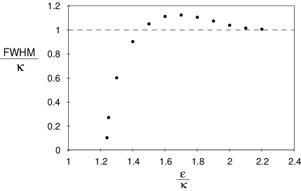
FIG. 6.: Dependence of the width of the peak at zero frequency in the squeezing spectrum as a function of the input driving strength for N=1. The following parameters were used: $(g,\kappa,\gamma)/2\pi$ = $(38.0,8.7,3.0)$ MHz. The FWHM has been normalized by the cavity decay rate, $\kappa$.

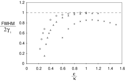
FIG. 7.: Dependence of the width of the peak at zero frequency in the squeezing spectrum for three different spontaneous emission rates as a function of the input driving strength for N=2 and the following parameters: $(g,\kappa,\gamma_{1},\gamma_{2},\gamma_{3})/2\pi$ = $(38/\sqrt{2},8.7,3.0,1.0,0.5)$ MHz. The FWHM for each plot has been normalized by its respective spontaneous emission rate, $\gamma_{i}$. The circles are for $\gamma=0.5$, the triangles are for $\gamma=1.0$, and the x’s are for $\gamma=3.0$. Notice the difference in driving strengths, $\epsilon/\kappa$, between this figure and the previous one.

C High Intensity

A large positive peak in the spectrum of squeezing appears at zero frequency when we increase the strength of the driving field to the case when there is about one-tenth of a photon in the cavity, and two atoms interacting with the mode. Negative peaks appear at a frequency less than that of the coherent coupling, $g$, between the atoms and the field. Figure 8i shows the result of directly solving the master equation with the quantum regression theorem.

The connection between the spectrum of squeezing and the time domain fluctuations shows that the field undergoes an exponential damping which is not present for the weaker driving fields (see Fig. 8ii). The careful reader may think there is a slight problem in saying that the connection between the spectrum of squeezing and the third order correlation function still holds in these stronger fields. We will show, from the results of a quantum trajectory simulation in section VI.b, that the qualitative behaviour of the fluctuations remain the same. Therefore the third order correlation function provides a legitimate method for studying the spectrum of squeezing beyond the weak field approximation.

We can get a preliminary understanding of the strong field spectrum of squeezing from the OB work of Reid and Walls [24]. They showed that in the optically bistable regime of a strongly driven, on resonance cavity, the spectrum of squeezing is a Lorentzian centered at zero frequency. We understand that this peak comes from the coupling of the cavity mode to its environment, but until the recent experiments of Foster et al. [2], we have had no motivation to understand the origin of this peak in the time domain.

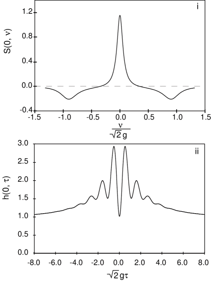
FIG. 8.: i. Spectrum of Squeezing and ii. its inverse fourier transform for two atom system under a stronger driving field. This figure shows the influence of the peak at zero frequency on the fluctuations in the time domain. $X=18.1$ and $(g,\kappa,\gamma)/(2\pi)=(38.0/\sqrt{2},8.7,3.0)$ MHz.

VI discussion

We have analyzed some of the many trajectories which go into making up the third order correlation functions shown in the last section by setting $r\approx 1$ in Eq. (36). We first begin by reviewing some results in the weak field regime and then we consider the more interesting regime of stronger driving intensities.

A Weak Field Trajectories

Figure 9 shows examples of the conditional field evolution calculated quantum trajectory simulations. Figure 9i shows the evolution of the field following the detection of a photon escaping through the cavity mode and Fig. 9ii shows the field evolution following the spontaneous emission of a photon out the side of the cavity. We used the following realistic parameters from the work of Foster et al [2, 3]: $(g,\kappa,\gamma)/2\pi$=$(38.0,8.7,3.0)$ MHz. This means that the system is in the strong coupling regime for one and two atoms.

The basic dynamical mechanism which describes these two results can be traced back to the change of the state $|\psi\rangle$ following a collapse operation of the type found in Eq. 17. We now consider the reduction of the equilibrium state of the cavity QED system on the occasion of a triggering photon detection (see Fig. 1). Defining $\hat{A}_{\theta}\equiv(\hat{a}{\rm{exp}}(-i\theta)+\hat{a}^{\dagger}{\rm{exp}}(i\theta))/2$, where $\hat{a}$ is the annihilation operator for the cavity field and $\theta$ is the BHD phase, we consider the quadrature amplitude, $\hat{A}_{0^{\circ}}$, in phase with the steady state of the field $\lambda\equiv\langle\hat{a}\rangle$. For weak excitation, and assuming fixed atomic positions $\{\vec{r}_{j}\}$, to second order in $\lambda$ the equilibrium state is the pure state [17, 18]

$$|\psi_{\rm{SS}}\rangle= [|0\rangle+\lambda|1\rangle+(\lambda^{2}/\sqrt{2})\alpha\beta|2\rangle+\cdots]|G\rangle$$ (39)

$$+ [\phi|0\rangle+\lambda\phi\beta|1\rangle+\cdots]|E\rangle+\cdots$$ (40)

where $|G\rangle$ is the one or two-atom ground state and $|E\rangle$ is for one atom in the excited state with all others in the ground state. We assume that all the atoms are coupled to the cavity mode with the same strength, $g$. The explicit form for $\phi,\alpha$ and $\beta$ follow from solving the master equation in the steady state [17]. They are

$$\phi=-\frac{2\sqrt{N}g}{\gamma}\lambda$$ (41)

$$\alpha=1-2C_{1}^{\prime},$$ (42)

$$\beta=\frac{1+2C}{1+2C-2C_{1}^{\prime}}$$ (43)

where $C\equiv NC_{1}$ and $C_{1}^{\prime}\equiv\frac{C_{1}}{(1+\gamma/2\kappa)}$.

After detecting the escaping photon, the conditional state is initially the reduced state $\hat{a}|\psi\rangle/\lambda$, which then relaxes back to equilibrium. The reduction and regression is traced by [17, 18]

$$|\psi\rangle\to\{|0\rangle+\lambda[1+\zeta f(\tau)]|1\rangle+\cdots\}|G\rangle+\cdots,$$ (44)

where

$$\zeta=-\frac{4C_{1}^{\prime}C}{1+2C-2C_{1}^{\prime}}$$ (45)

$$f(\tau)={\rm{exp}}(-(\kappa+\gamma/2)\tau/2)\!\left\{\cos\Omega\tau-\Phi\sin\Omega\tau\right\},$$ (46)

$$\Omega=\sqrt{{Ng^{2}-{1\over 4}\displaystyle}(\kappa-\gamma/2)^{2}}.$$ (47)

$$\Phi=-\frac{2\kappa+\gamma}{4\Omega}$$ (48)

Thus, the quadrature amplitude expectation makes the transient excursion $\langle\hat{A}_{0^{\circ}}\!\rangle\to\lambda[1+\zeta f(\tau)]$ away from its equilibrium value $\langle\hat{A}_{0^{\circ}}\!\rangle=\lambda$.

In contrast, an undetected spontaneous emission produces the reduced state $\hat{\sigma}^{-}|\psi\rangle/\lambda$, which sets up a completely different evolution as shown in Fig. 9ii. The reduction and regression in this case is again traced by Eq. (44) with the following replacements:

$$\zeta=\frac{2C_{1}^{\prime}}{1+2C-2C_{1}^{\prime}}$$ (49)

$$\Phi=\frac{2\kappa-\gamma}{4\Omega}+\frac{2Ng^{2}(\frac{q\beta}{\sqrt{2}}-1)}{\gamma\Omega(\beta-1)}$$ (50)

with $q=\sqrt{1-\frac{1}{N}}$.

These two distinct behaviors correspond fairly loosely to the regression to equilibrium observed in the step excitation in the field, Fig. 9i, and a step excitation in the atomic polarization, Fig. 9ii. Note the phase shift between the two responses. The steady state wavefunction determines the size of the steps.

$$\frac{\langle\hat{A}_{0^{\circ}(\rm cavity)}\rangle}{\langle\hat{A}_{0^{\circ}(\rm steadystate)}\rangle}=\alpha\beta$$ (51)

$$\frac{\langle\hat{A}_{0^{\circ}(\rm spontaneous)}\rangle}{\langle\hat{A}_{0^{\circ}(\rm steadystate)}\rangle}=\beta$$ (52)

We see from Eq. (43) that $\beta$ is a number greater than zero. The field will always remain positive when an atom spontaneously emits. As long as $g>\sqrt{\gamma(\kappa+\frac{\gamma}{2})/2}$, then through $\alpha$ (Eq. 42), the field will change sign when a photon escapes through the cavity mode.

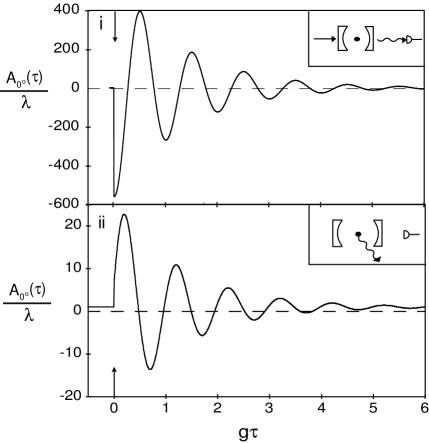
FIG. 9.: Regression of a cavity QED system back to steady state; N=1, low intensity i. after the detection of a photon escaping out of the cavity mode ii. after the escape of a photon through spontaneous emission. The inset shows the sequence of events in terms of the cavity QED system and the detector. The parameters used are the same as in Fig. 3.

The parameters used to create the plots in Fig. 9 are the same as those used in Fig. 3. Except for the residual shot noise in Fig. 3i, these two plots are in agreement with each other for $\tau>0$.

B High Field Trajectories

The weak field calculations of section VI.a make it clear that in the strong coupling regime a cavity emission will always produce a negative shift in the field. In order for us to observe fields of the type in Fig. 8ii and spectrum of squeezing of the type in Figs. 4, 5 and 8i we must find a mechanism which causes the expectation of the cavity field to jump positive after a cavity emission.

It follows from Eq. (40) that the ratio of the probability for a spontaneous emission to the probability for a cavity emission from steady state is

$$\frac{P_{\rm spont}}{P_{\rm cavity}}=2NC_{1}.$$ (53)

This implies that in the strong coupling regime it is more likely for the system to spontaneously emit out the sides of the cavity than directly into the cavity mode. Since we only begin a conditioned field measurement after a cavity mode emission, then it becomes necessary to consider what happens in the likely event of a cavity photon following a spontaneous emission.

Quantum trajectories allow one to follow the dynamics of the system under higher excitation. Figure 10 shows representative trajectories calculated from Eq. (36) when we have two atoms in the cavity and $r\approx 1$. The complete trajectory is a series of these excursions from the steady state well separated in time, and a returning to the steady state as shown. In Fig. 10i the evolution starts with a spontaneous emission (A) out the side of the cavity, followed at (B) by a photon escaping through the cavity mode that gets registered by the APD detector. Note how the field jumps positive and changes curvature with the escaping cavity photon. This is exactly the type of process which gives rise to the incoherent peak in the spectrum of squeezing.

We offer the following qualitative explanation of these types of events. The driving field ($\epsilon/\kappa$), atom-field coupling ($g$), and decay rates ($\kappa,\gamma$) are such that the system is in a regime where the cavity field is bunched. If we have a spontaneous emission event when the system has few excitations we return to the steady state value as in Fig. 3i. If the spontaneous emission event happens while in the bunched regime, followed by a cavity emission, then there are probably more excitations in the system. With one of the atoms removed from the system following the spontaneous emission, the probability for this energy to be in the cavity mode is increased. If we detect a cavity photon soon after the spontaneous emission, then we are probably in a regime where the intracavity field undergoes a large amplitude fluctuation, and the value of the cavity field is higher than the steady state value. This causes an upward jump in the expectation of the field. This is similar to the upward jump in the conditioned field of an OPO operated well below threshold [20]. In that system the conditioned steady state is small, since the system is most likely in the ground state, with a small probability of having a pair of photons in the cavity. When a photon emerges from the cavity one photon remains, and the conditioned average field rises. It is also clear that these types of events increase linearly with the number of atoms in the cavity, since the ratio of spontaneous emission events to cavity loss events is $2NC_{1}$.

If we drive the same system much harder the time evolution of the conditional field shows multiple jumps, some from spontaneous emission and some from escapes through the mode. The dynamics get very complicated and we show an example in Fig. 10ii for illustration, but the general trend remains, that the average value of the field is much larger than the steady state in such cases.

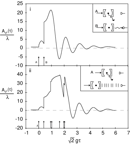
FIG. 10.: A quantum trajectory simulation which shows the time evolution of the field back to steady state after the detection of a photon. i. A spontaneous emission event followed by a cavity emission which starts the averaging process. ii. A spontaneous emission event followed by many cavity emission events. The inset shows the sequence of events in terms of the cavity QED system and the detector. Both figures were prepared with the following parameters: $N=2$, $X=18.1$, $(g,\kappa,\gamma)/(2\pi)$ = $(38.0/\sqrt{2},8.7,3.0)$ Mhz.

Figure 10 demonstrates the power of studying the single trajectories and also provides the major result of this paper. We see that the field will have a noise background arising from the mean cavity field, on top of other quantum fluctuations, when one has a spontaneous emission event out the side of the cavity. This is usually followed by a series of cavity emissions. This effect depends strongly on the number of atoms in the system and also on the strength of the driving field. This can not be seen from a direct numerical solution of the master equation, but now, thanks to the wave-particle correlator unravelling of the master equation, we begin to see exactly how these squeezing spectra are degraded by the incoherent process of spontaneous emission.

The entire trajectory is a collection of events well separated in time of the type in Figs. 10i and 10ii. If we average over many random realizations of these different events with an initial cavity emission setting the trigger at $t=0$, then we recover the averaged conditioned field evolution. Figure 11 shows such an average field which after symmetrization and upon taking the Fourier transform leads to a spectrum which resembles the experimental observations qualitatively. This also shows a similar behaviour as the oscillation from Fig. 4ii and therefore a legitimate connection can still be made between the correlation function of Eq. 1 and the spectrum of squeezing slightly beyond the weak field regime.

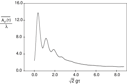
FIG. 11.: Conditioned field evolution calculated from 5000 realizations of a photon counting, quantum trajectory, simulation for N=2 and high intensity. $X=18.1$, $(g,\kappa,\gamma)/(2\pi)$ = $(38.0/\sqrt{2},8.7,3.0)$ Mhz.

C Time Symmetry

One result that we have only briefly mentioned is the fact that Fig. 3i is symmetric with respect to $\tau=0$ while the single events presented in Figs. 9 and 10 show a clear time asymmetry. This symmetry is recovered as a result of the BHD back action. The back action comes about because of the quantum superposition of both the local oscillator and cavity signal field (see Eq. (28)). It is not correct to think of these two fields as separable, a classical notion, but that each time a local oscillator photon is detected, it also effects the evolution of the cavity field. This implies that the conditional system state at time $t$ is correlated with the shot noise that has appeared over the recent past. Thus, through the “start” clicks (particle aspect), we postselect a subensemble of the shot noise which has in effect been filtered through the system’s dynamical response function (Hamiltonian evolution).

Quantum trajectories tend to reveal precisely those physical attributes they are trying to measure. By adding the homodyne detector we attempt to measure the fluctuations in the field amplitude, and when we do this these fluctuations appear in the averaged photocurrent before the arrival of a triggering photon.

D Future Work

By stating the problem in the time domain, we open the possibilities to apply quantum feedback theory [26, 27] in order to conditionally stabilize the atom-cavity system evolution against decoherence from the environment. This stabilization will not be optimal since the information obtained is limited to the quasimode leaking out of the cavity and any spontaneous emission event will be missed in the feedback loop. This calls for operating the cavity QED system in the low intensity regime to minimize spontaneous emission. We are currently investigating the theoretical and experimental requirements to develop such a program.

VII Conclusions

The conditional evolution of the field of a cavity QED system in the strong coupling regime shows non-classical behavior. This is purely quantal in nature and reflects the intrinsic dynamics triggered by the collapse of the wavefunction after the detection (conditioning) of a photon.

Looking at the time evolution of the conditional state as it regresses back to steady state we find that its behavior is far from random. When uninterrupted by other events, it follows a dynamic path that shows the coupling between the atom and the cavity and the significant excursion away from equilibrium brought back by a single quantum measurement. The spectrum of squeezing registers exactly the same behavior, but without the time and phase information critical to understanding the dynamics of the measurement process.

As we implement the measuring device used in the laboratory, we require an averaging process to observe the conditional evolution of the electromagnetic field. That evolution is non-classical. The phase is exactly $\pi$ from the driving field and it ocurrs when the intensity has a fluctuation up. This is contrary to all classical intuition that would say that then the field should have also a maximum, but in fact the field shows a minimum.

The presence of the homodyne measurement introduces back action into the system that then provides the foundation for the time symmetric wave-particle correlation function when third order correlations can be neglected.

The presence of other avenues for the interruption of the evolution back to steady state, such as spontaneous emission, modify the correlation function, decreasing its non-classicality, while at the same time modify the spectrum of squeezing around the origin with a peak that shows just the empty cavity width for the one atom case, or the spontantous emission width once the system is allowed to have more than one atom.

The wave-particle correlation function opens the door to further the study of quantum optical systems in the time domain that are necessary to understand better the possible realizations of quantum feedback systems.

VIII Acknowledgements

Work supported by NSF.

REFERENCES

- [1] H. J. Carmichael, H. M. Castro-Beltran, G. T. Foster, and L. A. Orozco, Phys. Rev. Lett. 85, 1855 (2000).
- [2] G. T. Foster, L. A. Orozco, H. M. Castro-Beltran, and H. J. Carmichael, Phys. Rev. Lett. 85, 3149 (2000).
- [3] G. T. Foster, Ph Dr Dissertation, SUNY Stony Brook 1999 (unpublished).
- [4] Squeezed states of the electromagnetic field, edited by H. J. Kimble and D. F. Walls, special issue of J. Opt. Soc. Am. B 4, 1450 (1987).
- [5] Squeezed light, edited by R. Loudon and P. L. Knight, special issue of J. Mod. Opt. 34, 709 (1987).
- [6] L. A. Lugiato in Progress in Optics, E. Wolf, ed. (North-Holland, Amsterdam, 1984), Vol. XXI, p. 69-216.
- [7] M. D. Reid and D. F. Walls, Phys. Rev. A 34, 4929 (1986).
- [8] M. G. Raizen, L. A. Orozco, M. Xiao, T. L. Boyd, and H. J. Kimble, Phys. Rev. Lett. 59, 198 (1987).
- [9] L. A. Orozco, M. G. Raizen, Min Xiao, R. J. Brecha, and H. J. Kimble, J. Opt. Soc. Am. B 4, 1490 (1987).
- [10] D. M. Hope, H. A. Bachor, P. J. Mamson, D. E. McClelland, P. T. H. Fisk, Phys. Rev. A 46 R1181 (1992).
- [11] H. J. Carmichael, Phys. Rev. Lett. 55, 2790 (1985)
- [12] P. R. Berman editor, Cavity Quantum Electrodynamics in Advances in Atomic Molecular, and Optical Physics, supplement 2 (Academic Press, Inc. San Diego, 1994).
- [13] G. Rempe, R. J. Thompson, R. J. Brecha, W. D. Lee, and H. J. Kimble, Phys. Rev. Lett. 67, 1727 (1991).
- [14] S. L. Mielke, G. T. Foster, and L. A. Orozco, Phys. Rev. Lett. 80, 3948 (1998).
- [15] G. T. Foster, S. L. Mielke, and L. A. Orozco, Phys. Rev. A 61, 053821 (2000).
- [16] J. P. Clemens and P. R. Rice, Phys. Rev. A 61, 063810 (2000).
- [17] H. J. Carmichael, R. J. Brecha, and P. R. Rice, Opt. Commun. 82, 73 (1991).
- [18] R. J. Brecha, P. R. Rice, and M. Xiao, Phys. Rev. A 59, 2392 (1999).
- [19] E. T. Jaynes, F. W. Cummings, Proc. IEEE 51, 89 (1963).
- [20] H. J. Carmichael, An Open Systems Approach to Quantum Optics, Lecture Notes in Physics, New Series m: Monographs, m18 (Springer-Verlag, Berlin, 1993).
- [21] M. Lax, Phys. Rev. 129, 2342 (1963); Phys. Rev. 157, 213 (1967).
- [22] M. B. Plenio and P. L. Knight, Rev. of Mod. Phys. 70, 101 (1998).
- [23] P.R. Rice and H.J. Carmichael, J. Opt. Soc. Am. B, 5, 1661 (1988).
- [24] M.D. Reid and D.F. Walls, Phys. Rev. A 32, 396 (1985).
- [25] H. J. Carmichael, Phys. Rev. A. 56, 5065 (1997), Sect. IV.
- [26] H.M. Wiseman and G.J. Milburn, Phys. Rev. Lett. 70, 548 (1993)
- [27] A. C. Doherty, S. Habib, K. Jacobs, H. Mabuchi, and S. M. Tan, to appear in Phys. Rev. A (2000).