Realization of quantum process tomography in NMR

Abstract

Quantum process tomography is a procedure by which the unknown dynamical evolution of an open quantum system can be fully experimentally characterized. We demonstrate explicitly how this procedure can be implemented with a nuclear magnetic resonance quantum computer. This allows us to measure the fidelity of a controlled-not logic gate and to experimentally investigate the error model for our computer. Based on the latter analysis, we test an important assumption underlying nearly all models of quantum error correction, the independence of errors on different qubits.

PACS: 03.67.-a, 06.20.Dk, 76.60.-k

I Introduction

Experimental characterization of the dynamical behavior of open quantum systems has traditionally revolved around semiclassical concepts such as coupling strengths, relaxation rates, and phase coherence times [1, 2]. However, quantum information theory tells us that so few parameters barely even begin to represent the full dynamics which quantum systems are capable of; for example, the evolution between two fixed times of a two-level quantum system (a qubit), coupled to an arbitrary reservoir, is described by twelve real parameters [3]. For a two qubit system, this number grows to $240$, and in general, for $n$ qubits it is $16^{n}-4^{n}$.

Of course, not all of these parameters are relevant for every physical process, and understanding the physics can boil down this huge parameter space to just a few important numbers. On the other hand, when the physical origins of a quantum process are not understood, or in question, it is invaluable to know that all these parameters can, in principle, be experimentally measured — albeit with exponential effort (in $n$) — using a procedure known as quantum process tomography. This method is a direct quantum extension of the classical concept of “system identification” which enables control of dynamical systems, and provides powerful measurement techniques for characterizing unknown systems. For closed systems, process tomography is the analog of determining the truth table of an unknown function; quantum-mechanically, this means the unitary transform involved in a quantum computation.

The procedure for quantum process tomography has been described in detail in the literature [3, 4, 5]. It relies upon the ability to prepare a complete set of quantum states ${\rho_{j}}$ as input to the unknown process ${\cal E}_{t}$, and the ability to measure the density matrices of the output quantum states from the process ${\cal E}_{t}(\rho)$. As a result, one obtains a complete “black box” characterization of ${\cal E}_{t}$. By systematically repeating this procedure for increasing process time $t$, one can also obtain a complete master equation description of the process [6].

This procedure seems to provide an ideal way to characterize and test quantum gates on a small number of qubits — for example, those realized using nuclear magnetic resonance (NMR) techniques [7, 8]. However, to date, this has not been practiced because of two problems: first, it is desirable to explicitly include the maximally mixed state as one of the $\rho_{j}$’s, so as to directly subtract its contribution, but such a state cannot be prepared by unitary actions alone. Second, one can only measure traceless observables, and thus one cannot obtain the entire output density matrix of a process.

Here, we show explicitly how these hurdles can be overcome, and demonstrate the use of these methods in addressing two outstanding issues in quantum computation: the fidelity of a quantum logic gate, the controlled-not gate, and the validity of the independent error model which is widely assumed for quantum error correction and fault tolerant computation.

The paper is divided into two major sections, which describe the theory, and our experiment. We begin with a review of quantum process tomography (QPT), then we explain our extensions to the basic procedure which enable QPT with NMR, and present theoretical models for decoherence in NMR. We then describe our experiment and procedure, and our two main experimental results.

II Theory

A Quantum process tomography

Quantum process tomography, as introduced by Chuang and Nielsen [3], can be summarized as follows. A general quantum operation on a quantum state $\rho$ is a superoperator $\cal E$, a linear, trace-preserving, completely positive map [9, 10, 11]. We consider only the case where $\cal E(\rho)$ has the same dimension as $\rho$. A common form for $\cal E$ is the operator-sum representation,

$${\cal E}(\rho)=\sum_{k}A_{k}\rho A_{k}^{\dagger}\,,$$ (1)

where $\sum_{k}A_{k}^{\dagger}A_{k}=I$. One can easily demonstrate the transformation to a fixed-basis expansion of the quantum operation such that the information about the process lies in a set of coefficients $\chi_{mn}$ instead of a set of operators. In this form, $\cal E$ maps an initial density matrix $\rho$ according to

$${\cal E}(\rho)=\sum_{m,n}\chi_{mn}A_{m}\rho A_{n}^{\dagger}\,.$$ (2)

In this expression, the $A_{m}$ are a basis for operators on the space of density matrices, and $\chi$ is a positive Hermitian matrix with elements $\chi_{mn}$. In the following, we will omit explicit summations and adopt the convention that repeated indices are summed over. Because of the restriction that $\cal E$ must preserve the trace of $\rho$, $\chi$ contains $N^{4}-N^{2}$ independent parameters for an $N$ dimensional system (for $n$ spins, $N=2^{n}$).

Let the $N^{2}$ matrices $\rho_{j}$ be a basis for density matrices. Applying $\cal E$ to this basis gives

$${\cal E}(\rho_{j})=\lambda_{jk}\rho_{k}\,.$$ (3)

Using quantum state tomography [12], one can experimentally determine $\lambda_{jk}$, which fully specifies $\cal E$. To determine $\chi$ from $\lambda$, we define $\beta$ by

$$A_{m}\rho_{j}A_{n}^{\dagger}=\beta^{mn}_{jk}\rho_{k}\,,$$ (4)

which is fully specified by the choice of $A_{m}$ and $\rho_{j}$. Then one can show that

$$\beta^{mn}_{jk}\chi_{mn}=\lambda_{jk}\,.$$ (5)

We may think of $\beta$ as a matrix and $\lambda$ and $\chi$ as vectors, with $mn$ a composite column index and $jk$ a composite row index; then $\beta\vec{\chi}=\vec{\lambda}$. Using the pseudoinverse $\kappa$ of $\beta$ (also called the Moore-Penrose generalized inverse), which may be computed independent of measurement results, we have

$$\vec{\chi}=\kappa\vec{\lambda}\,.$$ (6)

B QPT in NMR

Implementing QPT in high temperature NMR presents two main obstacles. First, the part of the system which can be manipulated by unitary operations is but a small deviation from a maximally mixed state. Second, one can only measure traceless observables, and the scaling of these observables with respect to the traceful part of the system is not immediately known. Fortunately, both of these hurdles can be overcome.

The Hamiltonian for solution NMR is well approximated by

$$H=-\hbar\omega_{j}{Z_{j}\over 2}+hJ_{jk}{Z_{j}Z_{k}\over 4}\,,$$ (7)

where

$$Z_{j}=\left(\matrix{1&0\cr 0&-1}\right)$$ (8)

is the Pauli operator for the $j$th spin along the direction of the magnetic field, $\omega_{j}$ is its Larmor frequency, and the sign of the first term is chosen so that the ground state is spin up. The second term represents a small scalar coupling between spins known as the $J$-coupling.

The initial state of an NMR quantum computer is the thermal equilibrium state with density matrix

$$\rho_{\infty}={e^{-H/k_{B}T}\over{\rm tr}(e^{-H/k_{B}T})}=cI+\Delta_{\infty}\,,$$ (9)

where $c=2^{-n}$ for a system of $n$ spins (so that ${\rm tr}(\rho_{\infty})=1$) and $\Delta_{\infty}$ is traceless. In general, we refer to the traceless part of any density matrix $\rho$ as the deviation density matrix. If we neglect the small coupling between spins and consider high temperature with respect to the Larmor frequencies, the equilibrium density matrix is approximately

$$\rho_{\infty}\approx c\left(I+{\hbar\omega_{j}Z_{j}\over 2k_{B}T}\right)\,.$$ (10)

By performing unitary operations on the system, we may rotate the $\omega_{j}Z_{j}$ deviation, allowing us to prepare a linearly independent set of inputs $\rho_{j}$. Because all of the interesting information will lie in this deviation, we would like to be able to prepare an input with no deviation (i.e., the maximally mixed state), so that we may directly subtract the contribution of the identity. Such an input clearly cannot be prepared by unitary means. However, the maximally mixed state can be prepared from the thermal state by applying a $\pi\over 2$ pulse followed by a uniformly spatially varying RF pulse. Different parts of the sample experience different amounts of rotation, so that the ensemble is effectively dephased to the maximally mixed state.

The second difficulty can be handled by calibrating measurements to the known initial state of the system. By state tomography, we can measure $\tilde{\Delta}=d\Delta_{\infty}$, where the constant $d$ is arbitrary — it depends in detail on the gain of the amplifiers, the efficiency of the RF coils, etc. But the initial deviation density matrix is known to be $c{\hbar\omega_{j}Z_{j}\over 2k_{B}T}$. Hence we may calibrate our apparatus by determining the value $d$ that makes the measured $\tilde{\Delta}/d$ closest to the theoretical $\Delta_{\infty}$. In practice, we effect this calibration by normalizing all measurements (integrals of spectral peaks) for spin $j$ to a reference measurement taken on that spin (a $\pi\over 2$ pulse applied to the thermal state) multiplied by $c{\hbar\omega_{j}\over 2k_{B}T}$.

C Decoherence primitives

Decoherence of a single NMR spin in solution is generally characterized by two well-known processes, amplitude damping and phase damping. Here, we present these processes, as well as generalizations to multiple spins. To facilitate the description of multiple simultaneous processes, we describe amplitude damping and phase damping as semigroups in terms of their generators.

Assuming that a quantum operation can be described by a norm continuous one-parameter semigroup, given a superoperator ${\cal E}_{t}$ satisfying the stationarity and Markovity condition ${\cal E}_{s}{\cal E}_{t}={\cal E}_{s+t}$ [13], its generator $\cal Z$ is defined as [14]

$${\cal Z}(\rho)=\lim_{t\to 0}{{\cal E}_{t}(\rho)-\rho\over t}\,.$$ (11)

The generators have the advantage that they easily describe the simultaneous action of multiple processes. In particular, we have the Trotter formula [14, 15],

$${\cal E}^{(1+2)}_{t}=\lim_{n\to\infty}\left({\cal E}^{(1)}_{t/n}{\cal E}^{(2)}_{t/n}\right)^{n}\,,$$ (12)

where

$${\cal Z}^{(1+2)}={\cal Z}^{(1)}+{\cal Z}^{(2)}\,,$$ (13)

with obvious generalization to more than two processes.

Furthermore, we may return to the superoperator form by exponentiating the generator [14]:

$${\cal E} = \lim_{n\to\infty}\left(1-{t\over n}{\cal Z}\right)^{-n}$$ (14)

$$= e^{{\cal Z}t}\,.$$ (15)

This exponentiation may be defined by its Taylor series in the case of interest where $\cal Z$ is bounded. To implement exponentiation in practice, it is useful to work with a manifestly linear representation, i.e., that of Eq. (3). In this case, a superoperator and its generator can be represented as matrices which have the property that composition of superoperators corresponds to matrix multiplication. Then the procedure of Eq. (14) corresponds to matrix exponentiation.

We now consider the single-qubit versions of phase and amplitude damping. For further discussion of these processes, including operator-sum representations, see [16]. We write the density matrix of a qubit as

$$\rho=\left(\matrix{{\rho_{00}}&{\rho_{01}}\cr{\rho_{10}}&{\rho_{11}}}\right)\,.$$ (16)

Phase damping can be thought of as a consequence of random phase kicks. It acts on a qubit as

$${\cal E}^{\rm PD}_{t}(\rho)=\left(\matrix{{\rho_{00}}&{e^{-\gamma t}\rho_{01}}\cr{e^{-\gamma t}\rho_{10}}&{\rho_{11}}}\right)\,,$$ (17)

for some damping rate $\gamma$; i.e., it has a generator which acts as

$${\cal Z}^{\rm PD}(\rho)=-\gamma\left(\matrix{0&\rho_{01}\cr\rho_{10}&0}\right)\,.$$ (18)

Ordering the matrix elements of $\rho$ in the vector $(\rho_{00},\rho_{01},\rho_{10},\rho_{11})^{T}$ (which effectively defines the basis used in Eq. (3)), we have

$${\cal Z}^{\rm PD}=\left(\matrix{0&0&0&0\cr 0&-\gamma&0&0\cr 0&0&-\gamma&0\cr 0&0&0&0}\right)\,.$$ (19)

Generalized amplitude damping is a process whereby the qubit may exchange energy with a reservoir at some fixed temperature. It acts on a qubit as

$${\cal E}^{\rm GAD}_{t}(\rho)=\left(\matrix{{k_{1}\rho_{00}+k_{2}\rho_{11}}&{e^{-\Gamma t/2}\rho_{01}}\cr{e^{-\Gamma t/2}\rho_{10}}&{k_{3}\rho_{00}+k_{4}\rho_{11}}}\right)\,,$$ (20)

where $k_{2}\equiv(1-\bar{n})(1-e^{-\Gamma t})$, $k_{3}\equiv\bar{n}(1-e^{-\Gamma t})$, $k_{1}\equiv 1-k_{3}$, and $k_{4}\equiv 1-k_{2}$, with $\Gamma$ a damping rate and $\bar{n}$ a temperature parameter. Its generator acts as

$${\cal Z}^{\rm GAD}=-\Gamma\left(\matrix{\bar{n}&0&0&\bar{n}-1\cr 0&{1\over 2}&0&0\cr 0&0&{1\over 2}&0\cr-\bar{n}&0&0&1-\bar{n}}\right)\,,$$ (21)

Computing the fixed point of this process, we find that we may interpret it as occuring at a temperature

$$k_{B}T={\Delta E\over\log{1-\bar{n}\over\bar{n}}}\,,$$ (22)

where $\Delta E$ is the splitting between the ground and excited states of the system.

Heuristically, we expect phase damping to describe the $T_{2}$ (dephasing) process of NMR. Similarly, generalized amplitude damping should describe the $T_{1}$ process of NMR, whereby a spin relaxes to align with the magnetic field. Note from the geometry of the Bloch sphere that amplitude damping necessarily includes loss of phase information, so it also contributes to the $T_{2}$ process. However, in typical systems, $T_{1}$ is much longer than $T_{2}$, so the contribution of amplitude damping to dephasing is small.

The simplest extension of these processes to a multiple-spin system is to allow the individual processes to act independently on each qubit. However, this is far from the most general scenario: the decoherence might be correlated. Although we have been unable to find a suitable correlated generalization of amplitude damping, we have incorporated a simple model of correlated phase damping due to Zhou into our analysis [17]. In this model, each spin experiences a random phase shift with zero mean. The amount of damping and the extent of correlation is defined by the covariance matrix of the phase shifts. By explicit calculation, one may easily find that this leads to a generator of the form

$${\cal Z}^{\rm CPD}={\rm diag} [ 0,-\gamma_{2},-\gamma_{1},-(\gamma_{1}+\gamma_{2}+\gamma_{3}),$$ (26)

$$-\gamma_{2},0,-(\gamma_{1}+\gamma_{2}-\gamma_{3}),-\gamma_{1},$$

$$-\gamma_{1},-(\gamma_{1}+\gamma_{2}-\gamma_{3}),0,-\gamma_{2},$$

$$-(\gamma_{1}+\gamma_{2}+\gamma_{3}),-\gamma_{1},-\gamma_{2},0]\,,$$

where $\gamma_{1}$ and $\gamma_{2}$ may be interpreted as rates for independent phase damping on spins $1$ and $2$, and $\gamma_{3}$ may be interpreted as a rate for correlated damping. Indeed, in the case $\gamma_{3}=0$, this model reproduces independent phase damping.

Our completed model has the generator

$${\cal Z}={\cal Z}^{J}+{\cal Z}^{\rm CPD}+{\cal Z}^{\rm GAD}_{1}+{\cal Z}^{\rm GAD}_{2}\,,$$ (27)

where a subscript indicates which spin is acted on and ${\cal Z}^{J}$ is the generator corresponding to the Hamiltonian

$$H^{J}=hJ{Z_{1}Z_{2}\over 4}\,.$$ (28)

In this Hamiltonian, the Zeeman terms are dropped from Eq. (7) because we work in a frame rotating at the Larmor frequencies of the two spins. To produce the model superoperator at any given time, we simply exponentiate Eq. (27).

III Experiment

We have implemented QPT on a system of two spins in an NMR apparatus. The experiments were performed at the IBM Almaden Research Center using an Oxford Instruments wide-bore magnet and a 500 MHz Varian Unity Inova spectrometer with a Nalorac triple resonance HFX probe. The sample was approximately $0.5~{}{\rm mL}$ of $200$ millimolar isotopically labeled chloroform (${}^{13}{\rm CHCl}_{3}$) in d6-acetone, where the two qubits were the proton (first spin) and carbon (second spin). This volume was chosen to make the sample fairly short, as this gave the most effective gradient pulse characteristics.

A Results: Gate fidelities

One application of quantum process tomography is to diagnose the accuracy of a quantum computation. When one applies a series of gates to perform the unitary operation $U$, the computer will actually perform a superoperator $\cal E$, which one hopes is close to $U$. That closeness can be captured by many distance measures — for example, the minimum gate fidelity, defined as

$$F=\min_{|\psi\rangle}\langle\psi|U^{\dagger}{\cal E}(|\psi\rangle\langle\psi|)U|\psi\rangle\,.$$ (29)

$F$ represents the smallest possible overlap between a state acted on by $U$ and the same state acted on by $\cal E$. Note that minimizing over pure states is sufficient because the fidelity is convex and because an arbitrary density matrix can be written as a convex sum of pure states.

Using QPT, we measured the minimum gate fidelity for a controlled-not operation, a well-known member of universal gate sets, with

$$U_{\sc cnot}=\left(\matrix{1&0&0&0\cr 0&1&0&0\cr 0&0&0&1\cr 0&0&1&0}\right)$$ (30)

The NMR pulse sequence chosen to implement this gate was

$$\bar{Y}_{1}X_{1}Y_{1}\bar{Y}_{2}d\left({1\over 2J}\right)Y_{2}X_{2}\,,$$ (31)

where time goes right to left, $X_{j}$ denotes a $\pi\over 2$ $x$ pulse on spin $j$, a bar denotes an inverse pulse, $d(\cdot)$ denotes a time evolution during which no pulses are applied, and $J=215~{}{\rm Hz}$ is the coupling constant for the scalar $J$-coupling between the spins. Procedures similar to those used in [18] were adopted to implement this pulse sequence. The pulse lengths were approximately $10-20~{}{\rm\mu s}$, sufficiently fast that the effect of $J$-coupling could be neglected during a pulse. Using quantum process tomography, we determined $\chi$ for this process, effectively determining $\cal E$. This result is shown in Fig. 1.

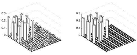
FIG. 1.: $\chi$ matrices for the controlled-not gate. The matrix on the left was experimentally measured by QPT, and that on the right is theoretical. Only the magnitudes of the matrix elements are shown; the phases also corresponded well between theory and experiment. The matrix element in the far left corner connects $II\leftrightarrow II$, and the elements are ordered as $II,XI,\ldots,YZ,ZZ$.

Given $\chi$, we may calculate gate fidelities. For the controlled-not gate, numerically minimizing over input states gives $F_{\sc cnot}=0.80\pm 0.04$.

This figure may be thought of as a rough benchmark for the quality of gates that can be implemented using current NMR quantum computers. However, several caveats should be addressed. Foremost, the preparation and readout steps performed to do the process tomography contribute to much of the error. Performing process tomography on a null computation ($U=I$), we find $F_{I}=0.90\pm 0.03$. The primary sources of error are most likely imperfect state preparation and imperfect state tomography due to imperfect pulse calibration and inhomogeneity of the RF fields [19].

Also, in a long computation, experimental results suggest that there may be a significant cancellation of errors [18]. Typically, the major contribution to the error introduced by an individual gate will be largely due to systematic errors rather than fundamentally irreversible decoherence. If the pulse sequence exhibits some degree of symmetry, these systematic errors may at least partially cancel. Thus the fidelity of a long sequence of gates cannot be deduced from the individual gate fidelities, though one would certainly expect it to be subadditive.

Of course, the minimum gate fidelity is a pessimistic standard; it may be more reasonable to consider the average gate fidelity. To numerically calculate the average fidelity, we must be able to sample uniformly from quantum states according to an appropriate probability measure. Although this problem is subtle for the case of mixed states, there is a straightforward choice for pure states: we take the unitary transform of a fixed state, where the unitary operator is chosen according to the Haar measure (the unique invariant measure on a Lie group). Using the procedure described in  [20], we calculated average fidelities with $10^{5}$ randomly chosen unitaries, giving $F^{\rm avg}_{\sc cnot}=0.955$ and $F^{\rm avg}_{I}=0.960$. Thus, the average fidelity is significantly better than the worst case; the error rate $1-F$ improves by about one order of magnitude.

B Results: Decoherence characterization

To characterize the decoherence occuring in the chloroform system, we used QPT to measure $\chi$ over the various relevant time scales. For an NMR spin, the relevant scales are $1\over 2J$, $T_{1}$, and $T_{2}$ [21]. We thus sampled at times given by $({1\over 2})^{j}{1\over 2\tilde{J}}$ for integers $j\in[0,4]$, $({1\over 2})^{j}\tilde{T}_{1}$ for $j\in[-1,4]$, and $({2\over 3})^{j}\tilde{T}_{2}$ for $j\in[0,9]$, where $\tilde{J}=215~{}{\rm Hz}$ is the known value of the $J$-coupling, $\tilde{T}_{1}=20~{}{\rm s}$ is a time scale on the order of $T_{1}$, and $\tilde{T}_{2}=0.5~{}{\rm s}$ is an intermediate time scale on the order of $T_{2}$.

By executing process tomography, we are able to determine $\chi$ as a function of time. However, $\chi$ is a large, complex collection of numbers that cannot be easily interpreted. To better understand the results, we fit the data to a model process, $\chi_{m}$, which hopefully provides a reasonable description of the relevant physics. Specifically, we use the model which results from exponentiating Eq. (27).

For each $\chi$, we determined the closest fit to our model by numerically minimizing ${\rm tr}[(\chi_{\rm m}-\chi)^{\dagger}(\chi_{\rm m}-\chi)]$, where $\chi_{\rm m}$ is a model superoperator derived from Eq. (27). This figure of merit was on the order of $5\%$ for most fits. The experimentally measured $\chi$ matrices as well as the corresponding fits $\chi_{m}$ are shown in Fig. 2 for three delay times.

Fitting the various rate parameters of $\chi_{m}$ as a function of time allows us to characterize the process. These fits are shown in Figs. 3–5. The error bars in these plots are computed numerically, and are derived solely from the statistics of the measurements and the fitting procedure.

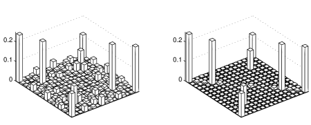
FIG. 2.: $\chi$ matrices for decoherence at various times. Matrices on the left are experimentally measured using QPT, and those on the right are fits to Eq. (27). Only the magnitudes of the matrix elements are shown, but their phases were also described well by the model. From top to bottom, $t=0.065~{}{\rm s},\ 0.5~{}{\rm s},\ 20~{}{\rm s}$. At $t=0.065~{}{\rm s}$, the time was chosen to be an integer number of $J$-coupling periods, which explains the lack of $IZ$, $ZI$, and $ZZ$ terms in the corners. At $t=0.5~{}{\rm s}$, note that the $IZ\leftrightarrow ZI$ terms arise from a combination of $J$-coupling and independent phase damping, not from correlated phase damping. At $t=20~{}{\rm s}$, note that the nonzero anti-diagonal terms found in the experiment do not appear in the fit even though such terms may arise in our amplitude damping model. Due to the details of the fitting procedure, the optimal fit matches large elements closely but does not capture the detail of the small anti-diagonal.

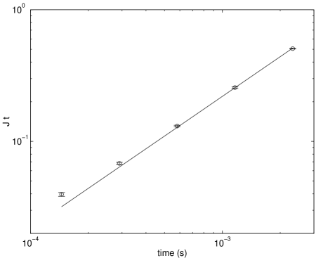
FIG. 3.: Determination of the strength of the scalar $J$-coupling between spins.

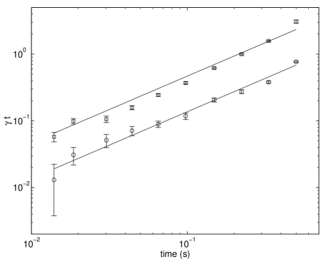
FIG. 4.: Determination of the phase damping rates $\gamma_{j}$. The circles represent $j=1$ (proton), and the squares represent $j=2$ (carbon). $\gamma_{3}$ is fitted to zero to within experimental uncertainty.

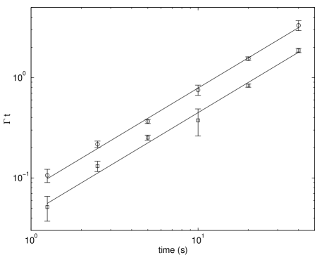
FIG. 5.: Determination of the amplitude damping rates $\Gamma_{j}$. The circles represent $j=1$ (proton), and the squares represent $j=2$ (carbon).

$J$	$220$$\thinspace\pm\thinspace$	$3~{}{\rm Hz}$
$\gamma_{1}^{-1}$	$0.73$$\thinspace\pm\thinspace$	$0.03~{}{\rm s}$
$\gamma_{2}^{-1}$	$0.21$$\thinspace\pm\thinspace$	$0.01~{}{\rm s}$
$\Gamma_{1}^{-1}$	$12.7$$\thinspace\pm\thinspace$	$0.3~{}{\rm s}$
$\Gamma_{2}^{-1}$	$22.4$$\thinspace\pm\thinspace$	$0.7~{}{\rm s}$

TABLE I.: Dynamical time scales for ${}^{13}{\rm CHCl}_{3}$, as measured by QPT. Recall that the proton is spin 1 and the ${}^{13}{\rm C}$ nucleus is spin 2. $\gamma_{3}$ is fitted to zero to within experimental uncertainty.

Our results are summarized in Table I. In addition to these data, we found the correlated phase damping rate $\gamma_{3}$ to be zero to within statistical precision. Unfortunately, insufficient precision was available to determine the amplitude damping temperature parameters $\bar{n}_{j}$. This is not a significant difficulty, as they are certain to be near $1\over 2$ for high temperature systems. The data are consistent with this value.

For comparison, the relevant decoherence parameters were measured by standard techniques. By the inversion-recovery technique, we found $T_{1}=18.5~{}{\rm s}$ for the proton and $T_{1}=21.1~{}{\rm s}$ for carbon. These values agree roughly with the time scales $\Gamma_{j}^{-1}$ for amplitude damping. Using the Carr-Purcell-Meiboom-Gill sequence, we found $T_{2}=4.7~{}{\rm s}$ for the proton and $T_{2}=0.26~{}{\rm s}$ for carbon. However, note that the relevant phase damping time scale is actually $T_{2}^{*}$, the time scale for relaxation due to magnetic field inhomogenity, which can be measured by fitting the free induction decay. By this method, we find $T_{2}^{*}=0.86~{}{\rm s}$ for the proton and $T_{2}^{*}=0.20~{}{\rm s}$ for carbon, values which agree more closely with the time scales $\gamma_{j}^{-1}$ measured by QPT.

As previously mentioned, the QPT preparation step is nonnegligible for the controlled-not gate fidelity experiment. However, this is not the case for the decoherence measurements: the time scales are long compared to the time to perform the QPT preparation, so small errors in the preparation are unimportant. For the experiments at short times to measure the parameter describing unitary evolution ($J$), the preparation is nonnegligible, but the operation is simple enough that we are still able to determine $J$ to within two standard deviations.

IV Conclusions

We have demonstrated the implementation of quantum process tomography to characterize the dynamics of a two-qubit NMR quantum computer. Such techniques should prove useful in the future for diagnosing quantum information processing devices. However, we should stress that due to the exponential size of $\chi$, QPT can only be used to characterize the dynamics of sufficiently small systems. For large systems, one may only be able to perform QPT on a small part of the total system, assuming independence from the rest of the system — an assumption which can, in turn, be checked using QPT.

Our measurements of gate fidelities underscore the difficulty of implementing highly accurate logic gates in NMR. These fidelity measurements suggest a per-gate error rate of the order of $10^{-1}$, in agreement with previous implementations of quantum algorithms [18]. It has been suggested that error rates of $10^{-2}$ can be achieved in solution NMR [22]. Indeed, if the previously dicussed cancellation of errors in a long sequence of gates leads to a $T_{2}$-limited computation (as observed in [18]), then an optimistic estimate of $T_{2}=1~{}{\rm s}$ and $J=100~{}{\rm Hz}$ leads to an approximate error rate of $10^{-2}$. Nevertheless, even this falls far short of the requirements for fault-tolerant quantum computing [23]: the least stringent estimates indicate a threshold for fault-tolerance of about $10^{-4}$ [24]. Clearly, the development of fault-tolerant NMR quantum computers will require substantially modified techniques. One might construct an alternative model for fault tolerance, perhaps based on topological properties [25]. However, with a conventional approach to fault tolerance, we will either need significant improvement of gate fidelity over what is currently achievable, specialization of fault tolerant protocols to the specific errors which occur in NMR, or both.

In turn, analyses of the threshold for fault-tolerant quantum computation typically involve an assumption of independent errors. Thus, for the experimental implementation of fault-tolerant computers, it is important to understand the error model in detail, and in particular, the extent to which the independence assumption holds. The results presented in Section III B show that this model is well-understood for the ${}^{13}{\rm CHCl}_{3}$ NMR system, and furthermore, that the errors are uncorrelated. The data are fit well by a combination of phase damping and independent generalized amplitude damping, with the phase damping essentially uncorrelated. Thus there exist simple computational systems in which an uncorrelated error model is reasonable.

However, note that there are systems which do exhibit correlated decoherence, namely those that exhibit “cross-relaxation” (in the terminology of NMR). For example, the simple two-spin proton-carbon system provided by sodium formate is known to possess cross-relaxation [26]. Investigation of such systems by QPT might be interesting not only for the purpose of quantum computing, but also for studying cross-relaxation in the context of conventional NMR.

V Acknowledgements

We thank Constantino Yannoni for sample preparation and Lieven Vandersypen and Matthias Steffen for experimental assistance. We also thank all of the above as well as Mark Sherwood and Xinlan Zhou for numerous enlightening discussions. During final preparation of the manuscript, AMC was supported by the Fannie and John Hertz Foundation. DWL was partially supported by the DARPA Ultrascale Program under contract DAAG55-97-1-0341, the IBM Graduate Fellowship program, and the Nippon Telegraph and Telephone Corporation (NTT).

REFERENCES

- [1] W. H. Louisell, Quantum Statistical Properties of Radiation (Wiley, New York, 1973).
- [2] C. W. Gardiner, Quantum Noise (Springer-Verlag, New York, 1991).
- [3] I. L. Chuang and M. A. Nielsen, J. Mod. Opt. 44, 2455 (1997).
- [4] J. F. Poyatos, J. I. Cirac, and P. Zoller, Phys. Rev. Lett. 78, 390 (1997).
- [5] D. W. Leung, Towards Robust Quantum Computation, Ph.D. thesis, Stanford University (2000).
- [6] V. Buzek, Phys. Rev. A 58, 1723 (1998).
- [7] N. Gershenfeld and I. L. Chuang, Science 275, 350 (1997).
- [8] D. G. Cory, A. F. Fahmy, and T. F. Havel, Proc. Natl. Acad. Sci. USA 94, 1634 (1997).
- [9] B. Schumacher, Phys. Rev. A 54, 2614 (1996).
- [10] M.-D. Choi, Linear Algebra and Its Applications 10, 285 (1975).
- [11] K. Kraus, States, Effects, and Operations: Fundamental Notions of Quantum Theory, Lecture Notes in Physics, Vol. 190 (Springer-Verlag, Berlin, 1983).
- [12] State tomography for infinite-dimensional systems was proposed in K. Vogel and H. Risken, Phys. Rev. A 40, 2847 (1989). See [16] for a review of the simpler finite-dimensional case.
- [13] We use multiplicative notation to stand for composition of superoperators. In other words, .
- [14] E. B. Davies, Quantum Theory of Open Systems (Academic Press, London, 1976); One-Parameter Semigroups (Academic Press, London, 1980).
- [15] H. F. Trotter, Proc. Am. Math. Soc. 10, 545 (1959).
- [16] M. A. Nielsen and I. L. Chuang, Quantum Computation and Quantum Information (Cambridge UP, Cambridge, 2000).
- [17] X. Zhou, private communication.
- [18] L. M. K. Vandersypen, M. Steffen, M. H. Sherwood, C. S. Yannoni, G. Breyta, and I. L. Chuang, Appl. Phys. Lett. 76, 646 (2000).
- [19] In an earlier experiment, we achieved the fidelities , . Unfortunately, we were unable to reproduce these results.
- [20] K. Życzkowski and M. Kuś, J. Phys. A 27, 4235 (1994); M. Poźniak, K. Życzkowski, and M. Kuś, J. Phys. A 31, 1059 (1998).
- [21] The time scales are not relevant because we work in a rotating frame, using a pair of local oscilators tuned to match the well-known Larmor frequencies.
- [22] D. G. Cory, R. Laflamme, E. Knill, L. Viola, T. F. Havel, N. Boulant, G. Boutis, E. Fortunato, S. Lloyd, R. Martinez, C. Negrevergne, M. Pravia, Y. Sharf, G. Teklemariam, Y. S. Weinstein, and W. H. Zurek, quant-ph/0004104 (2000).
- [23] P. W. Shor, in Proceedings, 37th Annual Symposium on Fundamentals of Computer Science, 56 (IEEE Press, Los Alamitos, 1996).
- [24] D. Gottesman, Stabilizer Codes and Quantum Error Correction, Ph.D. thesis, California Institute of Technology (1997); J. Preskill, Proc. R. Soc. London A 454, 385 (1998).
- [25] A. Yu. Kitaev, Fault tolerant quantum computation by anyons, quant-ph/9707021.
- [26] C. L. Mayne, D. W. Alderman, and D. M. Grant, J. Chem. Phys. 63, 2514 (1975).