Revised on

The non-relativistic Schrödinger equation with the linear and Coulomb potentials is solved numerically in configuration space using the relaxation method. The numerical method presented in this paper is a plain explicit Schrödinger solver which is conceptually simple and is suitable for advanced undergraduate research.

1 Introduction

This work came out of an undergraduate research project at the University of Wisconsin-Milwaukee. The analytical solution of the hydrogen atom is a typical topic in advanced undergraduate or beginning graduate quantum mechanics which utilizes the series expansion technique. The analytic solution does not only illustrate the mathematical approach of solving differential equations, it also provides a benchmark for testing numerical methods. Initially the numerical solution of the hydrogen atom was intended to offer the undergraduate students in our department (the second and third authors of this paper) an opportunity to learn the elements of scientific computation and basic research strategies. The students began by learning the theory of partial differential equations, linux programming in $C$, and basic numerical methods. In order to give the students a taste of original theoretical research, they were asked to check the eigenvalues generated by a Nystrom momentum space code from a new paper with the configuration space code which they helped to develop. This paper documents the $r$-space code for the numerical solution of the non-relativistic Schrödinger equation (NRSE) with the Coulomb and linear potentials. It is hoped that this work is helpful to those students and teachers who want to integrate numerical methods with a traditional quantum mechanics curriculum.

2 Schrödinger Equation in configuration Space

The basis of the wavefunction of the Schödinger equation in configuration space is taken to be

$$\phi_{lm}({\mathbf{r}})={R_{l}(r)\over r}\,Y_{lm}(\Omega)$$ (1)

The radial part of the equation for a hydrogen atom is [1]

$${d^{2}R_{l}\over dr^{2}}+\left[{2\mu\over\hbar}\left(E+{e^{2}\over r}\right)-{l(l+1)\over r^{2}}\right]R_{l}=0.$$ (2)

A computer cannot integrate $r$ from zero to infinity. Therefore we must map $[0,\infty)\to[0,1]$ by

$$r={x\over 1-x}$$ (3)

It implies that

$${dx\over dr}=(1-x)^{2}.$$ (4)

From now on, a new symbol for the radial wavefunction will be used, i.e. $y\equiv R_{l}$. To transform the Schrödinger equation to the new space, we first transform the second derivative,

$${d^{2}y\over dr^{2}} = {dx\over dr}{d\over dx}\left({dx\over dr}{dy\over dx}\right)$$ (5)

$$= (1-x)^{2}{d\over dx}\left((1-x)^{2}{dy\over dx}\right)$$

$$= (1-x)^{2}\left[2(1-x)\,{dy\over dx}+(1-x)^{2}{d^{2}y\over dx^{2}}\right]$$

By substituting Eq. [5] into Eq. [2] and letting $\hbar\to 1$ and

$$e^{2}={1\over 137},\qquad\mu=0.5107208\times 10^{6}\,eV,$$ (6)

in natural units, the Schrödinger equation is transformed as

$${d^{2}y\over dx^{2}}+{2\over 1-x}\,{dy\over dx}+{1\over(1-x)^{4}}\left[2\mu\left(E+{1-x\over x}\,e^{2}\right)-\left({1-x\over x}\right)^{2}l(l+1)\right]y=0.$$ (7)

With the benefit of hindsight, we know that the non-zero portion of the solution of Eq. [7] will be tightly bound to a narrow margin near $x\sim 0$. In order to improve the numerical accuracy and the quality of the plots, we like to focus on the non-zero portion of the solutions. A new configuration variable $z$ and a redefinition of $x$

$$z\equiv{r\over a_{0}},\qquad z={x\over 1-x},$$ (8)

where

$$a_{0}\equiv{\hbar^{2}\over\mu e^{2}}=2.6831879\times 10^{-4}\,eV^{-1},$$ (9)

are used to zoom into the small $x$ region. Eq. [7] is modified as

$${d^{2}y\over dx^{2}}+{2\over 1-x}\,{dy\over dx}+{1\over(1-x)^{4}}\left[2\mu\,a_{0}^{2}\left(E+{1-x\over x}\,{e^{2}\over a_{0}}\right)-\left({1-x\over x}\right)^{2}l(l+1)\right]y=0.$$ (10)

3 Relaxation Method

The shooting method typically shoots from one boundary point to another using Runga-Kutta integration. In the case of the Schrödinger equation, the boundary points at $x=0$ and $x=1$ are both singular. A one-point shoot will not converge when the code marches toward a singularity. A two-point shoot marches from both boundary points at $x=0$ and $x=1$ to match a third boundary point somwhere in between. Even if it works, two-point shoot requires too much a priori knowledge of the wavefunction. Furthermore any Runga-Kutta based alogrithms, such as the shooting methods, will fail under normal circumstances because either (1) the integration tends to blow up to infinity when shooting from $x=0$ or (2) the integration is identically zero when shooting from $x=1$, given the boundary conditions $y(1)=y^{\prime}(1)=0$. An embedded exponentially-fitted Runga-Kutta method [2] is reported to work. But it is beyond the scope of an undergraduate research project. The relaxation method, on the other hand, will in principle handle two singular boundary points. In this paper, we adapt the relaxation codes used in Numerical Recipes [9]. In order to establish a continuity between this paper and the said reference, the same notations are used.

The basic idea of the relaxation method is to convert the differential equation into a finite difference equation. Error functions are then considered. For instance, the error function at the $k$-th mesh point of the $j$-th differential equation (one of $N$ coupled differential equations)

$$\left.{dy_{j}\over dx}\right|_{x_{k}}=g(x_{k},y_{1},\dots,y_{N})$$ (11)

is simply

$$E_{j,k}=y_{j,k}-y_{j,k-1}-(x_{k}-x_{k-1})g(x_{k},x_{k-1},y_{1,k},y_{1,k-1},\dots,y_{N,k},y_{N,y-1}).$$ (12)

The difference of $E_{j,k}$ is approximated by a first order Taylor series expansion, such that

$$\sum^{N}_{n=1}S_{i,n}\Delta y_{n,k-1}+\sum^{2N}_{n=N+1}S_{i,n}\Delta y_{n-N,k}=-E_{i,k},$$ (13)

where

$$S_{i,n}={\partial E_{i,k}\over\partial y_{n,k-1}},\qquad S_{i,n+N}={\partial E_{i,k}\over\partial y_{n,k}}.$$ (14)

The crux of this paper is to show how the matrix elements $S_{i,k}$ of the non-relativistic Schrödinger equation are calculated and how to streamline the relaxation codes. The ranges of the sums in Eq [13] are split over $[1,N]$ and $[N+1,2N]$ because of the peculiarity of the relaxation codes used in Numerical Recipes. We will not delve into the details of the codes in this paper. Readers are encouraged to refer to Numerical Recipes for a full explanation. As a motivation, it suffices to say that the main idea of the relaxation method is to begin with initial guesses of $y_{j,k}$ and relax them to the approximately true values by calculating the errors $E_{i,k}$ to correct $y_{j,k}$ iteratively. $y_{j,k}$ are components of a solution vector in an $NM$-dimensional vector space. Intuitively we can think of the relaxation process as rotating an initial vector into another vector under the constraints of $E_{i,k}$. Since $y=0$ is a trivial solution, the relaxation process has a tendency to diminish those components of the solution vector that correspond to the wavefunction and its derivative. We will return to this point later in the paper.

Let $M-1$ be the number of mesh points and $h$ is step size, then

$$h={1\over M-1},$$ (15)

and

$$x_{k} = (k-1)h,$$ (16)

$$y_{k} \equiv y(x_{k}).$$ (17)

We define the vector $y_{i}$ as

$$\left\{\begin{array}[]{l l}&y_{1}=y\\ &y_{2}=y^{\prime}\\ &y_{3}=E\end{array}\right.$$

such that

$$y_{1}^{\prime} = y_{2}$$ (18)

$$y_{2}^{\prime} = -{2\over 1-x}\,y_{2}-{1\over(1-x)^{4}}\left[2\mu\,a_{0}^{2}\left(y_{3}+{1-x\over x}\,{e^{2}\over a_{0}}\right)-\left({1-x\over x}\right)^{2}l(l+1)\right]y_{1}$$ (19)

$$y_{3}^{\prime} = 0$$ (20)

A first order finite derivative at $x_{k}$ is given as

$$y_{k}^{\prime}={y_{k}-y_{k-1}\over h}.$$ (21)

In the relaxation formalism, $E_{i,k}$ are to be zeroed. In this case, it is easy to see that Eq. [18] can be rewritten as

$$E_{1,k}=y_{1,k}-y_{1,k-1}-{h\over 2}(y_{2,k}+y_{2,k-1}).$$ (22)

The corresponding $S_{1,j}$ $S$-matrix elements are

$$S_{1,1} = {dE_{1,k}\over dy_{1,k-1}}=-1,$$ (23)

$$S_{1,2} = {dE_{1,k}\over dy_{2,k-1}}=-{h\over 2},$$ (24)

$$S_{1,3} = {dE_{1,k}\over dy_{3,k-1}}=0,$$ (25)

$$S_{1,4} = {dE_{1,k}\over dy_{1,k}}=1,$$ (26)

$$S_{1,5} = {dE_{1,k}\over dy_{2,k}}=-{h\over 2},$$ (27)

$$S_{1,6} = {dE_{1,k}\over dy_{3,k}}=0.$$ (28)

Similarly, Eq. [19] is rewritten as

$$E_{2,k} = y_{2,k}-y_{2,k-1}+{2h\over 1-{x_{k}+x_{k-1}\over 2}}({y_{2,k}+y_{2,k-1}\over 2})+{h\over\left(1-{x_{k}+x_{k-1}\over 2}\right)^{4}}$$ (29)

$$\quad\times\left[2\mu\,a_{0}^{2}\left({y_{3,k}+y_{3,k-1}\over 2}+{1-{x_{k}+x_{k-1}\over 2}\over{x_{k}+x_{k-1}\over 2}}\,{e^{2}\over a_{0}}\right)\right.$$

$$\quad\qquad-\left.\left({1-{x_{k}+x_{k-1}\over 2}\over{x_{k}+x_{k-1}\over 2}}\right)^{2}\,l(l+1)\right]\,{y_{1,k}+y_{1,k-1}\over 2}.$$

The associating $S_{1,j}$ $S$-matrix elements are

$$S_{2,1} = {dE_{2,k}\over dy_{1,k-1}}$$ (30)

$$= {h\over 2\left(1-{x_{k}+x_{k-1}\over 2}\right)^{4}}\left[2\mu\,a_{0}^{2}\left({y_{3,k}+y_{3,k-1}\over 2}+{1-{x_{k}+x_{k-1}\over 2}\over{x_{k}+x_{k-1}\over 2}}\,{e^{2}\over a_{0}}\right)\right.$$

$$\qquad\qquad\qquad\qquad-\left.\left({1-{x_{k}+x_{k-1}\over 2}\over{x_{k}+x_{k-1}\over 2}}\right)^{2}\,l(l+1)\right],$$

$$S_{2,2} = {dE_{2,k}\over dy_{2,k-1}}$$ (31)

$$= -1+{h\over 1-{x_{k}+x_{k-1}\over 2}},$$

$$S_{2,3} = {dE_{2,k}\over dy_{3,k-1}}$$ (32)

$$= {h\mu\,a_{0}^{2}\over\left(1-{x_{k}+x_{k-1}\over 2}\right)^{4}}\,{y_{1,k}+y_{1,k-1}\over 2},$$

$$S_{2,4} = {dE_{2,k}\over dy_{1,k}}=S_{2,1},$$ (33)

$$S_{2,5} = {dE_{2,k}\over dy_{2,k}}$$ (34)

$$= 1+{h\over 1-{x_{k}+x_{k-1}\over 2}},$$

$$S_{2,6} = {dE_{2,k}\over dy_{3,k}}=S_{2,3}.$$ (35)

At last, Eq. [20] is rewritten as

$$E_{3,k}=y_{3,k}-y_{3,k-1},$$ (36)

and the associating $S_{3,j}$ matrix elements are

$$S_{3,1} = {dE_{3,k}\over dy_{1,k-1}}=0,$$ (37)

$$S_{3,2} = {dE_{3,k}\over dy_{2,k-1}}=0,$$ (38)

$$S_{3,3} = {dE_{3,k}\over dy_{3,k-1}}=-1,$$ (39)

$$S_{3,4} = {dE_{3,k}\over dy_{1,k}}=0,$$ (40)

$$S_{3,5} = {dE_{3,k}\over dy_{2,k}}=0,$$ (41)

$$S_{3,6} = {dE_{3,k}\over dy_{3,k}}=1.$$ (42)

At the first boundary point $x=0$, we have $n_{1}=1$. The boundary condition is $y(0)=0$. It translates to

$$E_{3,1}=y_{1,1}.$$ (43)

The only non-zero $S$-matrix element is

$$S_{3,4}=1.$$ (44)

At the second boundary point $x=1$, we have $n_{2}=2$. The boundary conditions are $y(1)=y^{\prime}(1)=0$, or equivalently

$$E_{1,M} = y_{1,M},$$ (45)

$$E_{2,M} = y_{2,M}.$$ (46)

The only non-zero matrix elements are

$$S_{1,4} = 1,$$ (47)

$$S_{2,5} = 1.$$ (48)

The hydrogen atom finite difference equation can be generalized to any Coulomb pentential by substituting $e^{2}\to\lambda_{C}$. To adapt the code to solve NRSE with a linear potential, the only modifications needed are

$${1-x\over x}\,e^{2}\to-{x\over 1-x}\,\lambda_{L},$$ (49)

in Eq. [19],

$${1-{x_{k}+x_{k-1}\over 2}\over{x_{k}+x_{k-1}\over 2}}\,e^{2}\to-{{x_{k}+x_{k-1}\over 2}\over 1-{x_{k}+x_{k-1}\over 2}}\,\lambda_{L}$$ (50)

in Eqs. [29,30], and the omission of all $a_{0}$ from the matrix elements.

4 Exact Solution of the Hydrogen Atom

The non-relativistic hydrogen atom is solved exactly by series expansion. The first few radial wavefunctions are found to be [1]

$$R_{10}(r) = {1\over\sqrt{\pi}}\,\gamma_{1}^{3\over 2}r\,e^{-\gamma_{1}r},$$ (51)

$$R_{20}(r) = {1\over\sqrt{\pi}}\,\gamma_{2}^{3\over 2}r\,(1-\gamma_{1}r)\,e^{-\gamma_{2}r},$$ (52)

$$R_{21}(r) = {1\over\sqrt{\pi}}\,\gamma_{2}^{5\over 2}r^{2}\,e^{-\gamma_{2}r},$$ (53)

where

$$\gamma_{n}\equiv{1\over n\,a_{0}}$$ (54)

With the redefinition of variable by Eqs. [8,9] and the omission of normalization constants, Eqs. [51–53] can be rewritten as

$$R_{10}(z) \sim z\,e^{-z},$$ (55)

$$R_{20}(z) \sim z\,(1-z)\,e^{-{z\over 2}},$$ (56)

$$R_{21}(z) \sim z^{2}\,e^{-{z\over 2}}.$$ (57)

Eqs. [55–57] will be used to test the relaxation codes in Section [6].

5 Exact $S$-state Solution for the Linear Potential

The $S$-state eigenvalue of the non-relativistic Schrödinger equation with a linear potential can be solved exactly in configuation space. We shall use the analytic results to check our numerical results. The non-relativistic Schrödinger equation can be written as

$$\left({d^{2}\over dr^{2}}+{2\over r}\,{d\over dr}\right)\,R-2\mu[\lambda_{L}\,r-E]\,R=0.$$ (58)

Let $S\equiv r\,R$, then Eq. [58] can be simplified as

$${d^{2}\over dr^{2}}S-2\mu[\lambda_{L}\,r-E]S=0.$$ (59)

Define a new variable

$$x\equiv\left({2\mu\over\lambda_{L}^{2}}\right)^{1\over 3}[\lambda_{L}r-E],$$ (60)

such that Eq. [58] can be transformed as

$$S^{\prime\prime}-xS=0,$$ (61)

which is the Airy equation. The solution which satisfies the boundary condition $S\to 0$ as $x\to\infty$ is the Airy function ${\rm Ai}(x)$. It is easy to show that the eigen-energy formula is

$$E_{n}=-x_{n}\,\left({\lambda_{L}^{2}\over 2\mu}\right)^{1\over 3},$$ (62)

where $x_{n}$ is the $n$-th zero of the Airy function counting from $x=0$ along $-x$. In reference [10], the values $\lambda_{L}=5$ and $\mu=0.75$ are used. In this case, the eigen-energy formula is

$$E_{n}=-2.554364772\,x_{n}.$$ (63)

6 Numerical Results

The matrix elements in the routine difeq have been calculated in section 3. All but the main driver subroutines are left intact. The intial guesses of the wavefunction and its derivative in the main driver program are just the square of the sine function and its derivative. The codes of the modified driver programs,bohr.c and linear.c, and the associating difeq.c are listed in the appendix of this paper. All the codes are written in $C$.

For large number of mesh points ($1000\leq N\leq 10000$), the code generates smooth wavefunctions and energies which do not correspond to any eigen modes. An explicit Schrödinger solver is known to be conditionally unstable [3, 4]. This kind of instabilities motivates numerical schemes such as the Numrov method [5], the symplectic scheme [6], microgenetic algoritm [7], and others [8]. For smaller number of mesh points ($40\leq N\leq 100$), it is observed that the relaxed eigenvalues are largely similar to the initial guesses and that the smoothness of the relaxed eigenfunctions is very sensitive to the initial guesses of the eigenvalue values. Therefore we adopt the criterion that the smoothness of the relaxed wavefunction picks out an initial guess as the correct eigenvalue when the number of mesh points is small enough. This criterion has certain a priori appeal because we expect a real physical wavefunction to be smooth. The reason for using the initial guess instead of the relaxed eigenvalue is based on the observation that the former is more accurate than the latter when the code is calibrated using exact results. Table [1] illustrates the motivation of the smoothness criterion. The combination of a small number of mesh points and the smoothness criterion is the simplest way to make the relaxation code workable as an explicit Schrödinger solver.

Figs. [1–3] compare the relaxed and exact wavefunctions of the hydrogen atom for the first few quantum numbers. The relaxed wavefunction typically has a vanishingly small amplitude. It is explained by the tendency of the relaxation routine to relax the wavefunction to the trivial solution $\psi=0$. In order to compare the relaxed and exact wavefunctions, the amplitude of the diminishing relaxed wavefunction is rescaled to match the exact wavefunction. Despite the large descrepancies between the relaxed and exact wavefunctions of the hydrogen atom in Figs. [1,2], both the relaxed and exact wavefunctions share the same basic features. Both relaxed wavefunctions satisfy the smoothness criterion. However, there are some difficulties in obtaining a smooth relaxed wavefunction for Fig. [3]. The relaxed wavefunction in this case also has an unwelcomed kink on the right hand side of the plot, which the exact wavefunction does not show. Hence the relaxed and exact wavefunctions do not share the same features in this case. The discrepancy here is mostly due to degeneracy. The eigen-energy formula of the hydrgon atom [1]

$$E_{nl}=-{e^{2}\over 2\,a_{0}}\,{1\over(n+l)^{2}}$$ (64)

reveals the degeneracy over the $n$ and $l$ quantum states. For example, $E_{21}=E_{30}$ such that the wavefunctions of these two states are degenerate by virtue of having the same eigenvalue. In principle, any linear combination of the degenerate solution vectors also satisfies the finite difference equation Eq. [10]. It also means that the relaxed wavefunction can be any linear combination of the degenerate wavefunctions. This problem will plague the numerical solutions of all degenerate states at higher $n$ and $l$. Imperfect wavefucntions is not a liability when the goal is to calculate the eigenvalues in the simplest possible way. In this case, the relaxed wavefunction is used merely as a guide to pick out the correct eigenvalue and not as a final product.

The situation of the numerical solution of the linear potential is slightly better. Figs [4,5] illustrate the relaxed wavefunctions of a linear potential compared to the exact wavefunctions. The wavefunctions of a linear potential are not degenerate. The relaxation method is expected to be relatively successful in the absence of degeneracy. In this paper, we use $\lambda_{L}=5\,{\rm GeV}$ and $\mu=0.75\,{\rm GeV}$. Table [2] lists the eigenvalues of the first few $l$ values in the case of the linear potential.

7 Conclusion

In this paper, we show how to circumvent the problem of conditional instability associating with an explicit Schrödinger solver when the relaxation method is used. The relaxation code with the combination of small number of mesh points and the smoothness criterion gives good approximate eigenvalues in both the linear and Coulomb potential cases. The role of the relaxed wavefunction is simply to guide the selection of the correct eigenvalue and is not used as an answer. More accurate eigenvalues can be obtained by solving the momentum space integral equation using the Nystrom method [11]. In this work, we have solved only the non-relativistic Schrödinger equation with the linear and Coulomb potentials. In the case of a relativistic equation, the Hamiltonian contains a kinetic term $\sqrt{p^{2}+m^{2}}-m$ which is difficult to solve numerically with $r$-space codes. The $p$-space solution using the Nystrom method on the other hand has the advantages of stability, accuracy and robustness over the $r$-space solution using the relaxation or shooting methods. For these reasons, we prefer the $p$-space codes over the $r$-space codes for production purposes. Nevertheless, the $r$-space code is useful in checking the $p$-space results whenever the former is available. The numerical $r$-space calculation is a natural starting point for students to learn scientific computation because they would have already seen the exact $r$-space solutions in a traditional quantum mechanics curriculum. Since the numerical solution of the hydrogen atom is not readily available in publications, it is hoped that the numerical method presented in this paper provides the simplest numerical scheme to supplement the discussion of the Schrödinger equation in an advanced undergraduate or beginning graduate quantum mechanics course.

8 Acknowledgment

We thank our advisor Prof. John W. Norbury for motivating this project.

9 Appendix

9.1 Non-relativistic Hydrogen Atom

bohr.c is a driver program for solving the non-relativistic hydrogen atom using the relaxation method. The inputs are $n$ (the principal quantum number), $l$ (the orbital angular momentum quantum number), $E$ (the initial guess of the ground state eigen-energy of the hydrogen atom which is approximately -13.6) and $scale$ (a scale factor to adjust the amplitude of the solution). The output is a file bohr.dat which contains the relaxed wavefunction.

/* bohr.c */

#include <stdio.h>
#include <math.h>
#include "difeq.c"
#include "/recipes/c/solvde.c"
#include "/recipes/c/bksub.c"
#include "/recipes/c/pinvs.c"
#include "/recipes/c/red.c"
#define NRANSI
#include "/recipes/c/nrutil.h"
#include "/recipes/c/nr.h"
#include "/recipes/c/nrutil.c"
#define NE 3
#define M 101
#define NB 1
#define NSI NE
#define NYJ NE
#define NYK M
#define NCI NE
#define NCJ (NE-NB+1)
#define NCK (M+1)
#define NSJ (2*NE+1)
#define pi 3.1415926535897932384626433

int l,mpt=M;
float h,x[M+1],mu,e2,a0;

int main(void)  /* Program bohr.c */
{
Ψvoid solvde(int itmax, float conv, float slowc, float scalv[],
ΨΨint indexv[], int ne, int nb, int m, float **y, float ***c,
ΨΨfloat **s);
Ψint i,itmax,k,indexv[NE+1],n;
Ψfloat conv,deriv,sinpx,cospx,q1,slowc,scalv[NE+1],eigen,guess;
Ψfloat **y,**s,***c,max,scale;
ΨFILE *fp;

Ψmu=0.5107208e6;
Ψe2=7.297353e-3;
Ψa0=1.0/mu/e2;
Ψy=matrix(1,NYJ,1,NYK);
Ψs=matrix(1,NSI,1,NSJ);
Ψc=f3tensor(1,NCI,1,NCJ,1,NCK);
Ψitmax=100;
Ψconv=1.0e-5;
Ψslowc=1.0;
Ψh=1.0/(M-1);
Ψprintf("\nn, l, E, scale = ");
Ψscanf("%d%d%f%f",&n,&l,&guess,&scale);
Ψindexv[1]=1;
Ψindexv[2]=2;
Ψindexv[3]=3;
Ψfor (k=1;k<=(M-1);k++) {
ΨΨx[k]=(k-1)*h;
ΨΨsinpx=sin((n-l)*pi*x[k]);
ΨΨcospx=cos((n-l)*pi*x[k]);
ΨΨy[1][k]=sinpx*sinpx;
ΨΨy[2][k]=2.0*(n-l)*pi*cospx*sinpx;
ΨΨy[3][k]=guess/(l+n)/(l+n);
Ψ}
Ψx[M]=1.0;
Ψy[1][M]=0.0;
Ψy[3][M]=guess/(l+n)/(l+n);
Ψy[2][M]=0.0;
Ψscalv[1]=1.0;
Ψscalv[2]=1.0;
Ψscalv[3]=-guess/(l+n)/(l+n);
Ψsolvde(itmax,conv,slowc,scalv,indexv,NE,NB,M,y,c,s);
Ψeigen=-13.598289/(n+l)/(n+l);
Ψprintf("\nl\tE_in\t\tnumerical E\texact E\t\tnumerical-exact\n");
Ψprintf("%d\t%f\t%f\t%f\t%f\n\n",l,guess/(l+n)/(l+n),
Ψ       y[3][1],eigen,y[3][1]-eigen);
Ψfp=fopen("bohr.dat","w");
Ψmax=0.0;
Ψfor(i=1;i<=M;i++) if(fabs(y[1][i])>max) max=fabs(y[1][i]);
Ψfor(i=1;i<=M;i++) fprintf(fp,"%f\t%e\n",(i-1)*h,y[1][i]/max*scale);
Ψfclose(fp);
Ψfree_f3tensor(c,1,NCI,1,NCJ,1,NCK);
Ψfree_matrix(s,1,NSI,1,NSJ);
Ψfree_matrix(y,1,NYJ,1,NYK);
        return 0;
}
#undef NRANSI

The difeq.c code below defines the $S$-matrix elements of the finite difference equation of the non-relativistic hydrogen atom and is called by the relaxation subroutine solvde.c.

/* difeq.c for the hydrogen atom driver program */

extern int mpt,l;
extern float h,x[],mu,e2,a0;

void difeq(int k, int k1, int k2, int jsf, int is1, int isf, int indexv[],
Ψint ne, float **s, float **y)
{
  float xk,y1k,y2k,y3k;
Ψif (k == k1) {
Ψ  s[3][3+indexv[1]]=1.0;
Ψ  s[3][3+indexv[2]]=0.0;
Ψ  s[3][3+indexv[3]]=0.0;
Ψ  s[3][jsf]=y[1][1];
Ψ} else if (k > k2) {
ΨΨs[1][3+indexv[1]]=1.0;
ΨΨs[1][3+indexv[2]]=0.0;
ΨΨs[1][3+indexv[3]]=0.0;
ΨΨs[1][jsf]=y[1][mpt];
ΨΨs[2][3+indexv[1]]=0.0;
ΨΨs[2][3+indexv[2]]=1.0;
ΨΨs[2][3+indexv[3]]=0.0;
ΨΨs[2][jsf]=y[2][mpt];
Ψ} else {
ΨΨs[1][indexv[1]] = -1.0;
ΨΨs[1][indexv[2]] = -0.5*h;
ΨΨs[1][indexv[3]]=0.0;
ΨΨs[1][3+indexv[1]]=1.0;
ΨΨs[1][3+indexv[2]] = -0.5*h;
ΨΨs[1][3+indexv[3]]=0.0;
ΨΨxk=(x[k]+x[k-1])/2.0;
ΨΨy1k=(y[1][k]+y[1][k-1])/2.0;
ΨΨy2k=(y[2][k]+y[2][k-1])/2.0;
ΨΨy3k=(y[3][k]+y[3][k-1])/2.0;
ΨΨs[2][indexv[1]]=h/2.0/pow(1.0-xk,4.0)*
ΨΨ  (2.0*mu*a0*a0*(y3k+(1.0/xk-1.0)*e2/a0)
ΨΨ   -pow(1.0/xk-1.0,2.0)*l*(l+1));
ΨΨs[2][indexv[2]] = -1.0+h/(1.0-xk);
ΨΨs[2][indexv[3]]=h*mu/pow(1.0-xk,4.0)*y1k*a0*a0;
ΨΨs[2][3+indexv[1]]=s[2][indexv[1]];
ΨΨs[2][3+indexv[2]]=2.0+s[2][indexv[2]];
ΨΨs[2][3+indexv[3]]=s[2][indexv[3]];
ΨΨs[3][indexv[1]]=0.0;
ΨΨs[3][indexv[2]]=0.0;
ΨΨs[3][indexv[3]] = -1.0;
ΨΨs[3][3+indexv[1]]=0.0;
ΨΨs[3][3+indexv[2]]=0.0;
ΨΨs[3][3+indexv[3]]=1.0;
ΨΨs[1][jsf]=y[1][k]-y[1][k-1]-h*y2k;
ΨΨs[2][jsf]=y[2][k]-y[2][k-1]+2.0*h/(1.0-xk)*y2k+
ΨΨ  h/pow(1.0-xk,4.0)*(2.0*mu*a0*a0*(y3k+(1.0/xk-1.0)*e2/a0)
ΨΨΨΨ     -pow(1.0/xk-1.0,2.0)*l*(l+1))*y1k;
ΨΨs[3][jsf]=y[3][k]-y[3][k-1];
Ψ}
}

9.2 NRSE with a Linear Potential

linear.c is a driver program for solving the non-relativistic Schrödinger equation with a linear potential using the relaxation method. The inputs are $n$ (the principal quantum number), $l$ (the orbital angular momentum quantum number), $E$ (the initial guess of the eigen-energy) and $scale$ (a scale factor to adjust the amplitude of the wavefunction) The output is a file linear.dat which contains the relaxed wavefunction.

/* linear.c */

#include <stdio.h>
#include <math.h>
#include "difeq.c"
#include "/recipes/c/solvde.c"
#include "/recipes/c/bksub.c"
#include "/recipes/c/pinvs.c"
#include "/recipes/c/red.c"
#define NRANSI
#include "/recipes/c/nrutil.h"
#include "/recipes/c/nr.h"
#include "/recipes/c/nrutil.c"
#define NE 3
#define M 101
#define NB 1
#define NSI NE
#define NYJ NE
#define NYK M
#define NCI NE
#define NCJ (NE-NB+1)
#define NCK (M+1)
#define NSJ (2*NE+1)
#define pi 3.1415926535897932384626433

int l,mpt=M;
float h,x[M+1],mu,lambdal;

int main(void)
{
Ψvoid solvde(int itmax, float conv, float slowc, float scalv[],
ΨΨint indexv[], int ne, int nb, int m, float **y, float ***c,
ΨΨfloat **s);
Ψint i,itmax,k,indexv[NE+1],n;
Ψfloat conv,deriv,sinpx,cospx,q1,slowc,scalv[NE+1],max,e,scale;
Ψfloat **y,**s,***c;
ΨFILE *fp;

Ψmu=0.75;
Ψlambdal=5.0;
Ψy=matrix(1,NYJ,1,NYK);
Ψs=matrix(1,NSI,1,NSJ);
Ψc=f3tensor(1,NCI,1,NCJ,1,NCK);
Ψitmax=100;
Ψconv=1.0e-6;
Ψslowc=1.0;
Ψh=1.0/(M-1);
Ψprintf("\nn, l, E scale = ");
Ψscanf("%d%d%f%f",&n,&l,&e,&scale);
Ψindexv[1]=1;
Ψindexv[2]=2;
Ψindexv[3]=3;
Ψfor (k=1;k<=(M-1);k++) {
ΨΨx[k]=(k-1)*h;
ΨΨsinpx=sin(n*pi*x[k]);
ΨΨcospx=cos(n*pi*x[k]);
ΨΨy[1][k]=sinpx*sinpx;
ΨΨy[2][k]=2.0*n*pi*cospx*sinpx;
ΨΨy[3][k]=e;
Ψ}
Ψx[M]=1.0;
Ψy[1][M]=0.0;
Ψy[3][M]=e;
Ψy[2][M]=0.0;
Ψscalv[1]=1.0;
Ψscalv[2]=1.0;
Ψscalv[3]=e;
Ψsolvde(itmax,conv,slowc,scalv,indexv,NE,NB,M,y,c,s);
Ψfp=fopen("linear.dat","w");
Ψmax=0.0;
Ψfor(i=1;i<=M;i++) if (fabs(y[1][i])>max) max=fabs(y[1][i]);
Ψfor(i=1;i<=M;i++) fprintf(fp,"%f\t%f\n",(i-1)*h,y[1][i]/max*scale);
Ψfclose(fp);
Ψprintf("\nl\tE_i\t\tE_f\n");
Ψprintf("%d\t%f\t%f\n\n",l,e,y[3][1]);
Ψfree_f3tensor(c,1,NCI,1,NCJ,1,NCK);
Ψfree_matrix(s,1,NSI,1,NSJ);
Ψfree_matrix(y,1,NYJ,1,NYK);
        return 0;
}
#undef NRANSI

The difeq.c code below define the $S$-matrix elements of the finite difference equation of a non-relativistic Schrödinger equation with a linear potential and is called by the relaxation subroutine solvde.c.

/* difeq.c for the linear potential driver program */

extern int mpt,l;
extern float h,x[],mu,lambdal;

void difeq(int k, int k1, int k2, int jsf, int is1, int isf, int indexv[],
Ψint ne, float **s, float **y)
{
  float xk,y1k,y2k,y3k;
Ψif (k == k1) {
Ψ  s[3][3+indexv[1]]=1.0;
Ψ  s[3][3+indexv[2]]=0.0;
Ψ  s[3][3+indexv[3]]=0.0;
Ψ  s[3][jsf]=y[1][1];
Ψ} else if (k > k2) {
ΨΨs[1][3+indexv[1]]=1.0;
ΨΨs[1][3+indexv[2]]=0.0;
ΨΨs[1][3+indexv[3]]=0.0;
ΨΨs[1][jsf]=y[1][mpt];
ΨΨs[2][3+indexv[1]]=0.0;
ΨΨs[2][3+indexv[2]]=1.0;
ΨΨs[2][3+indexv[3]]=0.0;
ΨΨs[2][jsf]=y[2][mpt];
Ψ} else {
ΨΨs[1][indexv[1]] = -1.0;
ΨΨs[1][indexv[2]] = -0.5*h;
ΨΨs[1][indexv[3]]=0.0;
ΨΨs[1][3+indexv[1]]=1.0;
ΨΨs[1][3+indexv[2]] = -0.5*h;
ΨΨs[1][3+indexv[3]]=0.0;
ΨΨxk=(x[k]+x[k-1])/2.0;
ΨΨy1k=(y[1][k]+y[1][k-1])/2.0;
ΨΨy2k=(y[2][k]+y[2][k-1])/2.0;
ΨΨy3k=(y[3][k]+y[3][k-1])/2.0;
ΨΨs[2][indexv[1]]=h/2.0/pow(1.0-xk,4.0)*(2.0*mu*
ΨΨΨΨΨ(y3k+xk/(xk-1.0)*lambdal)
ΨΨΨΨΨ-pow(1.0/xk-1.0,2.0)*l*(l+1));
ΨΨs[2][indexv[2]] = -1.0+h/(1.0-xk);
ΨΨs[2][indexv[3]]=h*mu/pow(1.0-xk,4.0)*y1k;
ΨΨs[2][3+indexv[1]]=s[2][indexv[1]];
ΨΨs[2][3+indexv[2]]=2.0+s[2][indexv[2]];
ΨΨs[2][3+indexv[3]]=s[2][indexv[3]];
ΨΨs[3][indexv[1]]=0.0;
ΨΨs[3][indexv[2]]=0.0;
ΨΨs[3][indexv[3]] = -1.0;
ΨΨs[3][3+indexv[1]]=0.0;
ΨΨs[3][3+indexv[2]]=0.0;
ΨΨs[3][3+indexv[3]]=1.0;
ΨΨs[1][jsf]=y[1][k]-y[1][k-1]-h*y2k;
ΨΨs[2][jsf]=y[2][k]-y[2][k-1]+2.0*h/(1.0-xk)*y2k+
ΨΨ  h/pow(1.0-xk,4.0)*(2.0*mu*(y3k+xk/(xk-1.0)*lambdal)
ΨΨΨΨ     -pow(1.0/xk-1.0,2.0)*l*(l+1))*y1k;
ΨΨs[3][jsf]=y[3][k]-y[3][k-1];
Ψ}
}

Figure 1: The relaxed $n=1$, $l=0$ wavefunction of the non-relativistic hydrogen atom compared against the exact wavefunction. The numerical eigenvalue is $-13.59827\,{\rm eV}$, versus the exact value of $-13.598289\,{\rm eV}$.

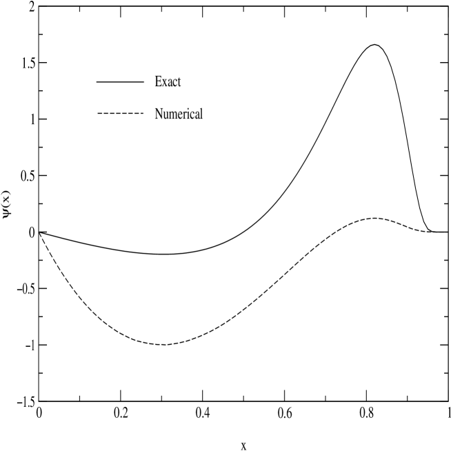
Figure 2: The relaxed $n=2$, $l=0$ wavefunction of the non-relativistic hydrogen atom compared against the exact wavefunction. The numerical eigenvalue is $-3.399750\,{\rm eV}$, versus the exact value of $-3.399572\,{\rm eV}$.

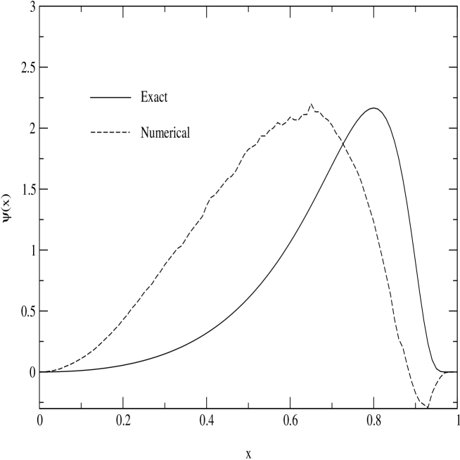
Figure 3: The relaxed $n=2$, $l=1$ wavefunction of the non-relativistic hydrogen atom compared against the exact wavefunction. The numerical eigenvalue is $-1.510056\,{\rm eV}$, versus the exact value of $-1.510921\,{\rm eV}$.

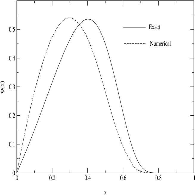
Figure 4: The relaxed $l=0$, $n=1$ state wavefunction of a non-relativistic Schrödinger equation with a linear potential using $\lambda_{L}=5\,{\rm GeV}$ and $\mu=0.75\,{\rm GeV}$. The numerical eigenvalue is $5.9719\,{\rm GeV}$, versus the exact value of $5.972379\,{\rm GeV}$. The relaxed wavefunction has been rescaled to match the exact wavefunction.

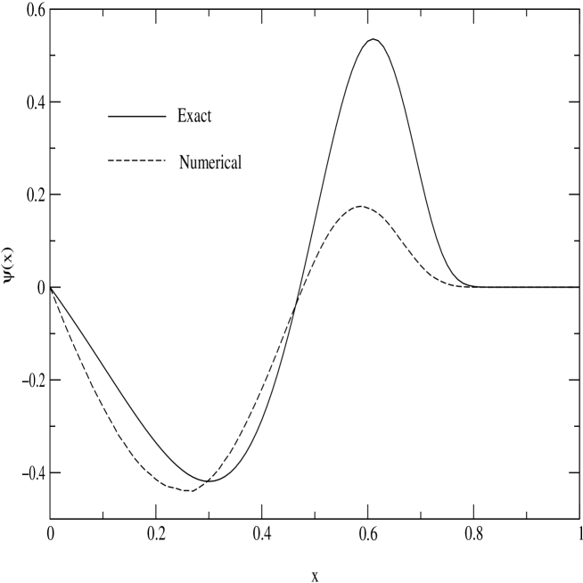
Figure 5: The relaxed $l=0$, $n=2$ state wavefunction of a non-relativistic Schrödinger equation with a linear potential using $\lambda_{L}=5\,{\rm GeV}$ and $\mu=0.75\,{\rm GeV}$. The numerical eigenvalue is $10.441\,{\rm GeV}$, versus the exact value of $10.442114\,{\rm GeV}$. The relaxed wavefunction has been rescaled to match the exact wavefunction.

Table 1: Comparisons among the inital guesses, the relaxed and exact eigenvalues of the non-relativistic hydrogen atom and the Schrödinger equation with a linear potential using $\lambda_{L}=5\,{\rm GeV}$, $\mu=0.75\,{\rm GeV}$.

			Coulomb
$n$	$l$	Initial	Numerical	Exact
1	0	-13.598270	-13.621142	-13.598289
2	0	-3.399750	-3.400535	-3.399572
2	1	-1.510056	-1.510060	-1.510921
			Linear
$n$	$l$	Initial	Numerical	Exact
1	0	5.9719	6.146734	5.972379
2	0	10.4410	10.418742	10.442114

Table 2: The numerical eigenvalues of the non-relativistic Schrödinger equation with a linear potential using $\lambda_{L}=5\,{\rm GeV}$, $\mu=0.75\,{\rm GeV}$ and $n=1$.

$l$	Numerical
0	5.9719
1	8.5850
2	10.8514
3	12.9020
4	14.9790
5	16.5845

References

- [1] W. Greiner, Quantum Mechanics: An Introduction (Frankfurt: Springer, 1989), 201.
- [2] G. Avdelas, T. E. Simos and J. Vigo-Aguiar, Computer Physics Communications, 131, 52 (2000).
- [3] T. Iitaka, Physical Review E, 49, 4684 (1994).
- [4] S. Succi, Physical Review E, 53, 1969 (1996).
- [5] G. Avdelas and T. E. Simos, Physical Review E, 62, 1375 (2000).
- [6] X. S. Liu, X. Y. Liu, Z. Y. Zhou, P. Z. Ding and S. F. Pan, International Journal of Quantum Chemistry, 79, 343 (2000).
- [7] H. Nakanishi and M. Sugawara, Chemical Physics Letters, 327, 429 (2000).
- [8] N. Watanabe and M. Tsukada, Physical Review E, 62, 2914 (2000).
- [9] W. H. Press, S. A. Teukosky, W. T. Vetterling, B. P. Flannery, Numerical Recipes in C (Cambridge: Cambridge, 1997).
- [10] J. W. Norbury, D. E. Kahana and K. M. Maung, Canadian Journal of Physics, 70, 86 (1992).
- [11] A. Tang and J. W. Norbury, to be published.