Abstract

Analytical expressions for the semiclassical dressed states and corresponding quasienergies are obtained for a two-level quantum system driven by a nonresonant and/or strong laser field in a coherent state. These expressions are of first order in a proper perturbative expansion, and already contain all the relevant physical information on the dynamical and spectroscopic properties displayed by these systems under such particular conditions. The influence of the laser field parameters on transition frequencies, selection rules, and line intensities can be easily understood in terms of the quasienergy-level diagram and the allowed transitions between the different semiclassical dressed states.

PACS number(s): 42.50.-p, 42.50.Ct

I. INTRODUCTION

The driven two-level model has been extremely useful in the study of the interaction of coherent light with atoms and molecules. Under resonant or near resonant conditions ($\Delta_{0}/\omega_{{\rm{L}}}\simeq 1$; with $\Delta_{0}$ being the transition frequency and $\omega_{{\rm L}}$ the driving field frequency) and not too strong laser fields ($\Omega_{0}/\omega_{{\rm{L}}}\ll 1$; with $\Omega_{0}$ being the Rabi frequency) one can invoke the rotating wave approximation and obtain an analytical description which is valid in the lowest order of the coupling constant. This approach, which is essentially the semiclassical Jaynes-Cummings model [1], corresponds to the regime most commonly encountered when considering atoms in the presence of a laser field.

The two-level model has also been used to describe interaction of matter with stronger or nonresonant laser fields. A first thorough study of the relevant effects of a strong oscillating field on a two-level quantum system was carried out by Autler and Townes [2], who making use of Floquet’s theorem derived a general solution in terms of infinite continued fractions. These authors applied their formulation to investigate the effect of an rf field on the $J=2\rightarrow 1\;l$-type doublet microwave absorption lines of molecules of gaseous OCS, obtaining good agreement with the experimental results. The practical usefulness of their analytical treatment decreases, however, as the oscillating field becomes stronger.

In another significant paper Shirley [3] proposed the Floquet theory as a convenient formalism for treating periodically driven quantum systems in the semiclassical approximation for the driving field. He then made use of this formalism (which replaces the time-dependent Hamiltonian with a time-independent Hamiltonian represented by an infinite matrix) to obtain, in particular, closed expressions for time-average resonance transition probabilities of a strongly-driven two-level system. Other works in the same spirit are those by Ritus [4] and Zeldovich [5]. The Floquet formalism has been further elaborated in many subsequent papers [6–10].

A different approach, especially suited to the nonperturbative regime, was followed by Cohen-Tannoudji and coworkers [11] to study the effects of a nonresonant linear rf field on the Zeeman hyperfine spectra of H¹ and Rb⁸⁷. These authors, using the dressed atom approach [12] which treats the external field as a single-mode quantum field, were able to account theoretically for the main features of the spectra, obtaining, in particular, the collapse of the spectral lines at the zeros of the proper zeroth-order Bessel function.

More recently, the driven two-level system has been used to study other interesting phenomena. For instance, this model can properly describe the effect of a driving laser field on the tunneling dynamics of low-lying electrons in a double quantum well [13]. In this regard, it has been shown [14,15] that an analytical solution which is zeroth order in the small parameter $\Delta_{0}/\omega_{{\rm L}}$ accounts correctly, over a wide parameter range, for the coherent suppression of tunneling that occurs in driven symmetric double-well potentials [16–19]. On the other hand, because of the fact that strongly driven two-level systems already display the main features of the high-order harmonic generation observed experimentally in the emission spectrum of atoms in very intense laser fields [20], this simple model has also been extensively used recently [21–28] to understand the basic mechanism underlying such a phenomenon [29]. In particular, first-order perturbative solutions have been derived for the equation of motion governing the dynamical evolution of the induced dipole moment [21–23]. A different approach has been followed in Ref. [30] to obtain a general first-order perturbative expression for the system time-dependent density operator, which is applicable regardless of the coupling strength value.

In this work we are interested in a complete analytical description in the energy domain of two-level quantum systems driven by far-off-resonance ($\Delta_{0}/\omega_{{\rm{L}}}\ll 1$) and/or strong laser fields ($\Omega_{0}/\omega_{{\rm{L}}}\gg 1$). As already mentioned, this regime, which corresponds to a parameter region where the semiclassical Jaynes-Cummings model is not applicable, has proved to be relevant in situations such as localization in a quantum double well or high-order harmonic generation in atomic and molecular species. None of the analytical treatments carried out so far in two-level systems driven by nonresonant and/or strong laser fields have arrived at such complete description, which not only requires the knowledge of the quasienergy-level diagram but also of the relevant Floquet states. In this regime the usual perturbative methods are no longer useful and one has to resort to a nonperturbative approach. Here we will develop a nonperturbative approach which is in the spirit of that by Cohen-Tannoudji and co-workers [11,12], but is based on the more manageable Floquet theory and, unlike previous approaches, goes up to first order in a proper perturbative expansion (associated with a transformed Hamiltonian). This order of approximation turns out to be the one required to obtain a complete account of the spectroscopic properties of the system. Our approach starts with a convenient unitary transformation and leads to nonperturbative closed analytical expressions for the Floquet states, which contain all the relevant physical information on this kind of systems. From these expressions we can obtain not only the selection rules (which in fact only depend on the system symmetry properties) but also analytical expressions for the intensities of the different spectral lines. Our formulation completes, in a sense, the analytical treatment of driven two-level systems by extending its range of applicability to include particular situations which correspond to a parameter region where the semiclassical Jaynes-Cummings model is not applicable.

In Sec. II we obtain the quasienergies and semiclassical dressed states (Floquet states) of a two-level quantum system driven by a nonresonant and/or strong laser field in a coherent state. Then, in Sec. III the system spectroscopic properties are analyzed in terms of its semiclassical dressed states and corresponding energy-level diagrams. In particular, the modifications induced in the system spectrum by the coupling with the laser field can be easily understood within this formalism. Finally, the main conclusions are summarized in Sec. IV.

II. SEMICLASSICAL DRESSED STATES

Consider a two-level system driven by a laser field in a coherent state. Under these circumstances the radiation field, which is assumed to be linearly polarized along the same direction as the system dipole operator, can be modeled by a classical electric field of frequency $\omega_{{\rm{L}}}$ and amplitude ${\bf E}_{0}$. The corresponding dimensionless Hamiltonian (in units of $\hbar\omega_{{\rm{L}}}$) is thus given, in the dipole approximation, by

$$H=\frac{\Delta_{0}}{2\omega_{{\rm{L}}}}\left(\sigma_{22}-\sigma_{11}\right)-\frac{\Omega_{0}}{\omega_{{\rm{L}}}}\cos\left(\tau\right)\left(\sigma_{12}+\sigma_{21}\right),$$ (1)

where $\Delta_{0}$ denotes the transition frequency between the excited state $|2\rangle$ and the ground state $|1\rangle$; $\sigma_{ij}\equiv|i\rangle\langle j|$ is the system transition operator; $\Omega_{0}\equiv E_{0}\mu/\hbar$ is the Rabi frequency, where $\mu$ (which is assumed to be real) denotes the dipole matrix element between $|1\rangle$ and $|2\rangle$; and $\tau=\omega_{{\rm{L}}}t$ is a dimensionless time variable.

This system is periodic in $\tau$ with the period $T=2\pi$ of the laser field. According to the Floquet theorem, the invariance of the Hamiltonian under the discrete time translation $\tau\rightarrow\tau+T$ guarantees that the general solution of the corresponding time-dependent Schrödinger equation can be expressed as a linear superposition of solutions of the type [3–7]

$$|\Psi_{j}(\tau)\rangle=e^{-i\varepsilon_{j}\tau}|\varphi_{j}(\tau)\rangle,\;\;\;\;\;\;(j=1,2),$$ (2)

where $\varepsilon_{j}$ are the (dimensionless) quasienergies and $|\varphi_{j}(\tau)\rangle=|\varphi_{j}(\tau+T)\rangle$ are the periodic Floquet states, which satisfy the eigenvalue equation

$$\left(H-i\frac{\partial}{\partial\tau}\right)|\varphi_{j}(\tau)\rangle=\varepsilon_{j}|\varphi_{j}(\tau)\rangle.$$ (3)

As can be easily seen, if $|\varphi_{j}(\tau)\rangle$ is a solution of Eq. (3) with quasienergy $\varepsilon_{j}$ then

$$|\varphi_{j}(\tau),n\rangle\equiv e^{in\tau}|\varphi_{j}(\tau)\rangle,$$ (4)

with $n$ being an arbitrary integer, is also a solution with quasienergy $\varepsilon_{j}+n$. The quasienergies are thus only defined mod $1$ (in units of $\hbar\omega_{{\rm{L}}}$).

Floquet states and quasienergies are the natural generalization of stationary states and energies of conservative Hamiltonians [3–7]. In particular, they can be shown to be the semiclassical counterpart of the dressed states appearing in a fully quantum treatment of the system in the presence of the quantized radiation field [12]. This reason makes them especially good for understanding the properties of periodically driven quantum systems in the energy domain. Information on transition frequencies, selection rules, and line intensities can be readily obtained from the form of the Floquet states and the quasienergy-level diagram.

Taking into account that according to the Floquet theorem any solution of the time-dependent Schrödinger equation can be written as

$$|\Psi(\tau)\rangle=\sum_{j}e^{-i\varepsilon_{j}\tau}\langle\varphi_{j}(0)|\Psi(0)\rangle\,|\varphi_{j}(\tau)\rangle,$$ (5)

and using the fact that $|\Psi(\tau)\rangle$ is given in terms of the evolution operator $U(\tau,0)$ by $|\Psi(\tau)\rangle=U(\tau,0)|\Psi(0)\rangle$, one immediately finds the following expression for the spectral decomposition of the one-period propagator [3–7],

$$U(T,0)=\sum_{j}e^{-i\varepsilon_{j}T}|\varphi_{j}(T)\rangle\langle\varphi_{j}(T)|,$$ (6)

where we have used the periodicity of $|\varphi_{j}(\tau)\rangle$ to identify $|\varphi_{j}(0)\rangle$ with $|\varphi_{j}(T)\rangle$. As Eq. (6) shows, the diagonalization of $U(T,0)$ provides the quasienergies and corresponding semiclassical dressed states at integer multiples of the laser period $T$. On the other hand, from the periodicity of the Floquet states and the relationship

$$|\varphi_{j}(\tau)\rangle=e^{i\varepsilon_{j}\tau}U(\tau,0)|\varphi_{j}(0)\rangle,$$ (7)

which is a direct consequence of Eq. (2), it follows that in order to gain a complete knowledge of the Floquet states at any time it suffices to determine the evolution propagator in the time interval $0<\tau\leq T$.

As already mentioned, in this paper we are mainly interested in the analysis of the spectroscopic properties of a two-level system driven by a far-off-resonance ($\Delta_{0}/\omega_{{\rm{L}}}\ll 1$) and/or strong laser field ($\Omega_{0}/\omega_{{\rm{L}}}\gg 1$) in terms of its semiclassical dressed states and quasienergy-level diagram. To this end we start by performing the following unitary transformation

$$U_{0}(\tau)=e^{-i\phi(\tau)\left(\sigma_{12}+\sigma_{21}\right)},$$ (8)

$$\phi(\tau)=\frac{\Omega_{0}}{\omega_{{\rm{L}}}}\sin\left(\tau\right),$$ (9)

which enables us to reformulate the problem in terms of a convenient small Hamiltonian, proportional to $\Delta_{0}/\omega_{{\rm{L}}}$. Indeed, using that

$$U_{0}(\tau)|1\rangle=\cos\phi(\tau)|1\rangle-i\sin\phi(\tau)|2\rangle,$$ (10)

$$U_{0}(\tau)|2\rangle=-i\sin\phi(\tau)|1\rangle+\cos\phi(\tau)|2\rangle,$$ (11)

one finds that the transformed Hamiltonian $H^{\prime}=U_{0}HU_{0}^{+}-iU_{0}\dot{U}_{0}^{+}$ takes the form

$$H^{\prime}=-\frac{\Delta_{0}}{2\omega_{{\rm{L}}}}\left\{\left[J_{0}\left(\zeta\right)+\alpha(\tau)\right]\left(\sigma_{11}-\sigma_{22}\right)+\beta(\tau)\left(\sigma_{12}-\sigma_{21}\right)\right\},$$ (12)

where

$$\alpha(\tau)\equiv\cos\left[2\phi(\tau)\right]-J_{0}\left(\zeta\right)=2\sum_{n=1}^{+\infty}J_{2n}\left(\zeta\right)\cos\left(2n\tau\right),$$ (13)

$$\beta(\tau)\equiv i\sin\left[2\phi(\tau)\right]=2i\sum_{n=0}^{+\infty}J_{2n+1}\left(\zeta\right)\sin\left[(2n+1)\tau\right],$$ (14)

$$\zeta\equiv\frac{2\Omega_{0}}{\omega_{{\rm{L}}}},$$ (15)

The Bessel functions $J_{n}\left(\zeta\right)$ entering the right hand side of Eqs. (13) and (14) come from the Fourier series expansion of the periodic coefficients $\alpha(\tau)$ and $\beta(\tau)$.

In the far-off-resonance regime the oscillating part of the above Hamiltonian can be considered as a small perturbation. In order to obtain a first-order expression for the system evolution operator it is most convenient to work in the interaction representation with respect to the zeroth-order Hamiltonian

$$H_{0}^{\prime}=-\frac{\Delta_{0}}{2\omega_{{\rm{L}}}}J_{0}\left(\zeta\right)\left(\sigma_{11}-\sigma_{22}\right).$$ (16)

In this representation the evolution operator $U_{{\rm I}}^{\prime}(\tau,0)=e^{iH_{0}^{\prime}\tau}U^{\prime}(\tau,0)$ satisfies the equation of motion

$$i\frac{d}{d\tau}U_{{\rm I}}^{\prime}(\tau,0)=\Delta H_{{\rm I}}^{\prime}\,U_{{\rm I}}^{\prime}(\tau,0),$$ (17)

where the perturbation $\Delta H_{{\rm I}}^{\prime}$ now reads

$$\Delta H_{{\rm I}}^{\prime}\equiv-\frac{\Delta_{0}}{2\omega_{{\rm{L}}}}\left[\alpha(\tau)\left(\sigma_{11}-\sigma_{22}\right)+\beta(\tau)\left(e^{-i\frac{\Delta_{0}}{\omega_{{\rm{L}}}}J_{0}\left(\zeta\right)\tau}\sigma_{12}-e^{i\frac{\Delta_{0}}{\omega_{{\rm{L}}}}J_{0}\left(\zeta\right)\tau}\sigma_{21}\right)\right].$$ (18)

The solution of Eq. (17) can be formally written as the following infinite series

$$U_{{\rm I}}^{\prime}(\tau,0)={\bf 1}-i\int_{0}^{\tau}d\tau_{1}\Delta H_{{\rm I}}^{\prime}(\tau_{1})+(-i)^{2}\int_{0}^{\tau}d\tau_{1}\int_{0}^{\tau_{1}}d\tau_{2}\Delta H_{{\rm I}}^{\prime}(\tau_{1})\Delta H_{{\rm I}}^{\prime}(\tau_{2})+\ldots$$ (19)

In principle, this is a perturbative expansion in the small parameter $\Delta_{0}/\omega_{{\rm{L}}}$. However, from the asymptotic behavior of the Bessel functions in the strong-field regime ($\zeta\equiv 2\Omega_{0}/\omega_{{\rm{L}}}\gg 1$), i.e. [31],

$$J_{n}\left(\zeta\right)\sim\left\{\begin{array}[]{ll}\sqrt{2/\pi\zeta}\cos\left(\zeta-n\pi/2-\pi/4\right)&\mbox{ if $n<\zeta$}\\ \left(e\zeta/2n\right)^{n}/\sqrt{2\pi n}&\mbox{ if $n>\zeta$}\end{array}\right.$$ (20)

it is not hard to see that, in this regime, the perturbation $\Delta H_{{\rm I}}^{\prime}(\tau)$ becomes of the order of $\Delta_{0}/\sqrt{\omega_{{\rm{L}}}\Omega_{0}}$. Consequently, our perturbative analysis turns out to be valid not only in the far-off-resonance regime ($\Delta_{0}/\omega_{{\rm{L}}}\ll 1$), but also in the regime where

$$\Delta_{0}/\omega_{{\rm{L}}}\ll\sqrt{\Omega_{0}/\omega_{{\rm{L}}}}\gg 1.$$ (21)

This means that in the case of intense driving fields, the present formalism, which is generally applicable under nonresonant conditions, can also describe the evolution of the quantum system under resonant or quasi-resonant conditions. Put another way, our perturbative analysis permits one to study analytically the behaviour of the driven system in a region of the parameter space which is beyond the range of applicability of the semiclassical Jaynes-Cummings model and where interesting phenomena such as coherent suppression of tunneling and high-order harmonic generation take place.

The evolution operator $U(\tau,0)$ associated with the Hamiltonian (1) can be written in terms of $U_{{\rm I}}^{\prime}(\tau,0)$ as

$$U(\tau,0)=U_{0}^{+}(\tau)U^{\prime}(\tau,0)U_{0}(0)=U_{0}^{+}(\tau)e^{-iH_{0}^{\prime}\tau}U_{{\rm I}}^{\prime}(\tau,0).$$ (22)

Substituting Eq. (18) into Eq. (19) and the latter into Eq. (22), one obtains, after performing the corresponding integration, the following first-order perturbative expression for the evolution operator

$$U(\tau,0)=U_{0}^{+}(\tau)e^{-iH_{0}^{\prime}\tau}\left\{{\bf 1}+i\frac{\Delta_{0}}{\omega_{{\rm{L}}}}\left[\xi_{{\rm s}}\left(\tau\right)\left(\sigma_{11}-\sigma_{22}\right)+\eta(\tau)\sigma_{12}+\eta^{*}(\tau)\sigma_{21}\right]+O\left(\epsilon^{2}\right)\right\},$$ (23)

where

$$\xi_{{\rm s}}\left(\tau\right)\equiv\sum_{n=1}^{+\infty}J_{2n}\left(\zeta\right)\frac{\sin\left(2n\tau\right)}{2n},$$ (24)

$$\xi_{{\rm a}}\left(\tau\right)\equiv\sum_{n=0}^{+\infty}J_{2n+1}\left(\zeta\right)\frac{\cos\left[\left(2n+1\right)\tau\right]}{2n+1},$$ (25)

$$\eta(\tau)\equiv i\left[\xi_{{\rm a}}\left(0\right)-e^{-i\frac{\Delta_{0}}{\omega_{{\rm{L}}}}J_{0}\left(\zeta\right)\tau}\xi_{{\rm a}}\left(\tau\right)\right].$$ (26)

The s and a subscripts in the above formulae refer to the symmetrical or antisymmetrical behaviour of the corresponding factor under the time translation $\tau\rightarrow\tau+\pi$, and $\epsilon$ denotes the appropriate expansion parameter.

A similar expression has been derived by Frasca [32] using a different approach, valid in the strong-field limit, based on a series expansion dual to the Dyson series. The divergent secular terms appearing in such an approach were resummed by using renormalization group methods [33]. The approach followed in this paper, which is free of secular terms, demonstrates that the first-order evolution operator (23) is also generally applicable under nonresonant conditions. It is important to note, however, that our formula differs from Frasca’s by the factor $\exp\{-i[\Delta_{0}J_{0}(\zeta)/\omega_{{\rm{L}}}]\tau\}$ entering Eq. (26), which is absent in Ref. [32] and, as we shall see, proves to be essential in the subsequent derivation of the Floquet states.

In order to facilitate later manipulations it is convenient to rewrite $U(\tau,0)$ as the following unitary operator

$$U(\tau,0)=U_{0}^{+}(\tau)e^{-iH_{0}^{\prime}\tau}\exp\left\{i\frac{\Delta_{0}}{\omega_{{\rm{L}}}}\left[\xi_{{\rm s}}\left(\tau\right)\left(\sigma_{11}-\sigma_{22}\right)+\eta(\tau)\sigma_{12}+\eta^{*}(\tau)\sigma_{21}\right]\right\}\left[1+O\left(\epsilon^{2}\right)\right],$$ (27)

where the equality only holds up to first order in $\epsilon$. The one-period propagator thus takes the form

$$U(T,0)=e^{-i\frac{\Delta_{0}}{2\omega_{{\rm{L}}}}J_{0}\left(\zeta\right)T\sigma_{z}}\exp\left\{i\frac{\Delta_{0}}{\omega_{{\rm{L}}}}\left[\eta(T)\sigma_{-}+\eta^{*}(T)\sigma_{+}\right]\right\}\left[1+O\left(\epsilon^{2}\right)\right],$$ (28)

with

$$\sigma_{z}=\left(\sigma_{22}-\sigma_{11}\right),\;\;\;\;\sigma_{+}=\sigma_{21},\;\;\;\;\sigma_{-}=\sigma_{12}.$$ (29)

The operators $\sigma_{z},\sigma_{+},\sigma_{-}$ so defined satisfy the Lie Algebra of $SU(2)$. They are, in other words, the generators of the $SU(2)$ group. As is well known, any $SU(2)$ transformation can be expressed in terms of such generators in the form $\exp\left[i\left(a_{z}\sigma_{z}+a_{+}\sigma_{+}+a_{-}\sigma_{-}\right)\right]$. In particular, it can be proved that the one-period propagator (28) may be written, up to first-order in $\epsilon$, as

$$U(T,0)=\exp\left\{i\frac{\Delta_{0}}{\omega_{{\rm{L}}}}\left[-\frac{J_{0}\left(\zeta\right)T}{2}\sigma_{z}+\eta(T)\sigma_{-}+\eta^{*}(T)\sigma_{+}\right]\right\}\left[1+O\left(\epsilon^{2}\right)\right].$$ (30)

Diagonalization of this operator is now straightforward and leads to the following Floquet states at $\tau=T$

$$|\varphi_{1}(T)\rangle=|1\rangle-\frac{\Delta_{0}}{\omega_{{\rm{L}}}}\sum_{n=0}^{+\infty}\frac{J_{2n+1}\left(\zeta\right)}{2n+1}|2\rangle+O\left(\epsilon^{2}\right),$$ (31)

$$|\varphi_{2}(T)\rangle=\frac{\Delta_{0}}{\omega_{{\rm{L}}}}\sum_{n=0}^{+\infty}\frac{J_{2n+1}\left(\zeta\right)}{2n+1}|1\rangle+|2\rangle+O\left(\epsilon^{2}\right),$$ (32)

with corresponding quasienergies given by

$$\varepsilon_{1}=-\frac{\Delta_{0}}{2\omega_{{\rm{L}}}}J_{0}\left(\zeta\right)\left[1+O\left(\epsilon^{2}\right)\right]$$ (33)

$$\varepsilon_{2}=+\frac{\Delta_{0}}{2\omega_{{\rm{L}}}}J_{0}\left(\zeta\right)\left[1+O\left(\epsilon^{2}\right)\right]$$ (34)

It should be noticed that had we neglected the factor $\exp\{-i[\Delta_{0}J_{0}(\zeta)/\omega_{{\rm{L}}}]\tau\}$ entering Eq. (26), the corresponding one-period propagator would not differ from the zeroth-order expression $\exp\left(-iH_{0}^{\prime}T\right)$ and, consequently, after diagonalization we would obtain $|1\rangle$ and $|2\rangle$ as the Floquet states at $\tau=T$. Retaining such a factor is, therefore, essential in order to obtain a correct result.

The final expression for the semiclassical dressed states at any time $\tau$ can be derived from Eq. (7). Using the evolution operator given in Eq. (23) as well as the initial form of the Floquet states given in Eqs. (31) and (32), and retaining only terms up to first order in the expansion parameter one obtains, after some algebra,

$$\begin{array}[]{c}|\varphi_{1}(\tau)\rangle=\left\{\cos\phi(\tau)+i\frac{\Delta_{0}}{\omega_{{\rm{L}}}}\left[\xi_{{\rm s}}\left(\tau\right)\cos\phi(\tau)-\xi_{{\rm a}}\left(\tau\right)\sin\phi(\tau)\right]\right\}|1\rangle+\\ i\left\{\sin\phi(\tau)+i\frac{\Delta_{0}}{\omega_{{\rm{L}}}}\left[\xi_{{\rm s}}\left(\tau\right)\sin\phi(\tau)+\xi_{{\rm a}}\left(\tau\right)\cos\phi(\tau)\right]\right\}|2\rangle+O\left(\epsilon^{2}\right),\end{array}$$ (35)

$$\begin{array}[]{c}|\varphi_{2}(\tau)\rangle=i\left\{\sin\phi(\tau)-i\frac{\Delta_{0}}{\omega_{{\rm{L}}}}\left[\xi_{{\rm s}}\left(\tau\right)\sin\phi(\tau)+\xi_{{\rm a}}\left(\tau\right)\cos\phi(\tau)\right]\right\}|1\rangle+\\ \left\{\cos\phi(\tau)-i\frac{\Delta_{0}}{\omega_{{\rm{L}}}}\left[\xi_{{\rm s}}\left(\tau\right)\cos\phi(\tau)-\xi_{{\rm a}}\left(\tau\right)\sin\phi(\tau)\right]\right\}|2\rangle+O\left(\epsilon^{2}\right).\end{array}$$ (36)

These states are the first-order periodic Floquet states satisfying Eq. (3) with corresponding quasienergies given by Eqs. (33) and (34). This is the central result of this paper. All the relevant spectroscopic and dynamical properties that driven two-level quantum systems exhibit in the parameter range considered in this work can be inferred from the above analytical expressions. In other words, the Floquet states at first order already contain all the relevant physical information on the system properties in the region of parameter space where conditions $\Delta_{0}/\omega_{{\rm{L}}}\ll 1$ or $\Delta_{0}/\omega_{{\rm{L}}}\ll\sqrt{\Omega_{0}/\omega_{{\rm{L}}}}\gg 1$ hold.

As the above expressions reflect, both $|\varphi_{1}(\tau)\rangle$ and $|\varphi_{2}(\tau)\rangle$ are linear superpositions of the undriven atomic states $|1\rangle$ and $|2\rangle$ with oscillating weights whose mean values are basically determined by the dimensionless coupling parameter $\zeta$. For small $\zeta$ each Floquet state is dominated by a single atomic state (see Fig. 1a). The contribution of the other atomic state increases with $\zeta$ (Fig. 1b), reaching its maximum value at $\zeta=\pi$ (Fig. 1c). Beyond this point the weights of the two atomic states keep oscillating between the extreme values $0$ and $1$.

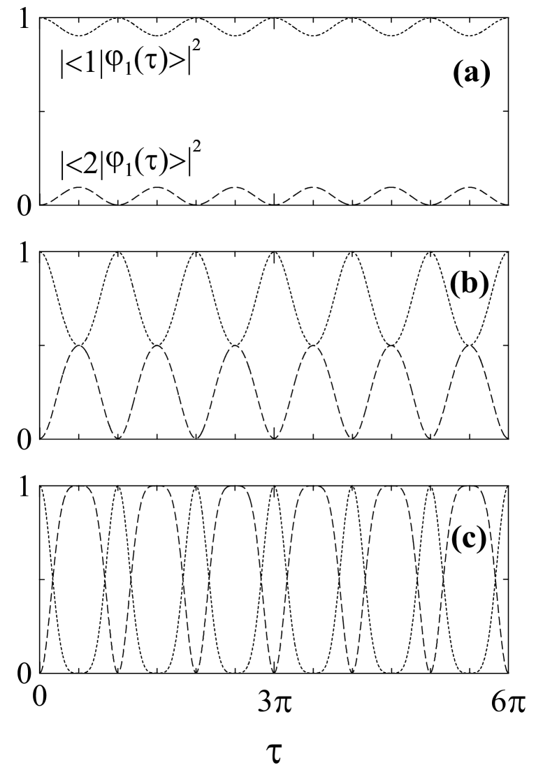
Figure 1: Weights of the undriven states $|1\rangle$ (dotted curves) and $|2\rangle$ (broken curves) in the Floquet state $|\varphi_{1}(\tau)\rangle$ as a function of $\tau$, for ${\Delta_{0}}/{\omega_{{\rm{L}}}}=0.1$; (a) $\zeta=\pi/5$; (b) $\zeta=\pi/2$; (c) $\zeta=\pi$. The corresponding weights in the Floquet state $|\varphi_{2}(\tau)\rangle$ are obtained from the above ones by interchanging the role of $|1\rangle$ and $|2\rangle$.

III. FLOQUET STATE SPECTROSCOPY

As already mentioned, Floquet states and quasienergies are the natural generalization of stationary states and energies of conservative Hamiltonians. In particular, they can be shown to correspond to the dressed states appearing in a fully quantum treatment of the system in the presence of the radiation field. This makes them particularly convenient to study the spectroscopic properties of a system driven by a classical external field.

The physical interpretation of Floquet states becomes more transparent by introducing an extended Hilbert space [6] consisting of all $T$-periodic functions $\chi_{i}\left({\bf r},\tau\right)$ normalizable with respect to the scalar product defined by

$$\ll\chi_{i}|\chi_{j}\gg=\frac{1}{T}\int_{0}^{T}d\tau\int d{\bf r\,}\chi_{i}^{*}\left({\bf r},\tau\right)\chi_{j}\left({\bf r},\tau\right).$$ (37)

A suitable basis in this extended Hilbert space is that composed of the Floquet states $|j,n\rangle$ corresponding to the undriven Hamiltonian,

$$|j,n\rangle\equiv e^{in\tau}|j\rangle,$$ (38)

where $j=1,2$ refers to the atomic state and the Fourier index $n$ is the semiclassical analog of the photon number appearing in a quantum treatment of the radiation field.

One of the main advantages of the semiclassical dressed state formalism is that the spectroscopic properties of periodically driven systems can be inferred from matrix elements of the corresponding transition operator in a way that closely resembles that commonly used when treating conservative Hamiltonians. In particular, the spectral lines of the allowed dipole transitions between different dressed states $|\varphi_{j}(\tau),m\rangle$ and $|\varphi_{i}(\tau),n\rangle$ have frequencies $\omega=\varepsilon_{j}-\varepsilon_{i}+m-n$ (in units of $\omega_{{\rm{L}}}$), and the corresponding intensities are proportional to

$$I_{in,jm}\equiv\left|\ll\varphi_{i}(\tau),n|\hat{d}|\varphi_{j}(\tau),m\gg\right|^{2}=\left|\ll\varphi_{i}(\tau)|\hat{d}e^{i(m-n)\tau}|\varphi_{j}(\tau)\gg\right|^{2},$$ (39)

where $\hat{d}=\mu\left(\sigma_{12}+\sigma_{21}\right)$ is the dipole operator.

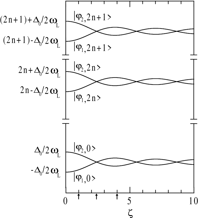
Figure 2: Quasienergy-level diagram for a few n-manifolds as a function of the dimensionless coupling parameter $\zeta$. The arrows in the $\zeta$-axis correspond to the three different physical situations considered in Fig. 3.

In our system these transition frequencies depend on the driving field parameters $\omega_{{\rm{L}}}$ and $\Omega_{0}$ entering the quasienergy expressions (33) and (34). This dependence can be observed in Fig. 2 where dressed-state levels corresponding to a few n-manifolds are plotted against the dimensionless coupling $\zeta$. This figure shows that level crossing occurs between the two levels in each n-manifold whenever the driving field parameters are tuned in such a way that the Bessel function $J_{0}(\zeta)$ vanishes. The existence of these level crossings, which is possible because, as will be seen, the corresponding states have different symmetry, leads to different spectroscopic properties depending on whether the system is located just at the crossing point or in either side.

The symmetry properties of the system can be used to obtain from expression (39) the selection rules for the allowed transitions. In particular, the states $|\varphi_{1}(\tau)\rangle$ and $|\varphi_{2}(\tau)\rangle$ given in Eqs. (35)–(36) turn out to be symmetric and antisymmetric, respectively, under the combined transformation

$$|1\rangle\rightarrow|1\rangle,\;\;\;\;\;|2\rangle\rightarrow-|2\rangle,\;\;\;\;\tau\rightarrow\tau+\pi,$$ (40)

which leaves the system Hamiltonian invariant. More generally, from this result and the definition (4) it follows that the Floquet states $|\varphi_{1}(\tau),n\rangle$ and $|\varphi_{2}(\tau),n+1\rangle$ are symmetric for even $n$ and antisymmetric for odd $n$. Since the dipole operator is antisymmetric under the above transformation, the matrix elements (39) between Floquet states with the same symmetry must vanish. Therefore, the selection rules for the allowed transitions between $|\varphi_{j}(\tau),m\rangle$ and $|\varphi_{i}(\tau),n\rangle$ are

$$\begin{array}[]{c}i=j,\;\;\;(m-n)\;{\rm odd},\\ i\neq j,\;\;\;(m-n)\;{\rm even}.\end{array}$$ (41)

Fig. 3 displays diagrams of the allowed transitions for the three different values of the parameter $\zeta$ indicated with arrows in Fig. 2. These values have been selected in order to explore the relevant physical situations. In Fig. 3a the driving field does not change the level ordering of the undriven system. As the $\zeta$ parameter increases level crossing occurs at the first zero of the Bessel function $J_{0}(\zeta)$ and after that, the original level ordering is inverted. These cases are illustrated in Figs. 3b and 3c, respectively.

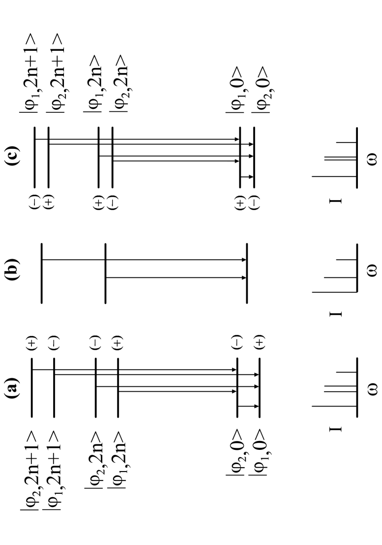
Figure 3: Allowed transitions between the different semiclassical dressed states for the three values of $\zeta$ considered in Fig. 2. The ($+$) and ($-$) symbols label symmetric and antisymmetric states, respectively. Only transitions ending in the $n=0$ manifold are plotted. The spectra at the bottom show the qualitative intensities I of these transitions as a function of the frequency $\omega$. Note that the most intense line in case (b) is a zero-frequency line corresponding to the transitions between the two degenerate states within the same n-manifold.

The transition between the two states within a given n-manifold ($i\neq j,\;m=n$) gives rise to a low frequency spectral line located at $\omega=\left|\Delta_{0}J_{0}(\zeta)/\omega_{{\rm{L}}}\right|$, whose intensity, after substitution of Eqs. (35)–(36) into Eq. (39), is found to be proportional to

$$I_{1n,2n}=\mu^{2}.$$ (42)

Note that the frequency of this transition goes to zero as the level crossing is approached (Fig. 3b), which reflects the fact that in such a case the dipole moment develops a constant component. On either side of the level crossing (Figs. 3a and 3c) the initial and final states of the transition are interchanged. This implies, for instance, that to the right of the first level crossing the transition initial state in the emission spectrum would correspond to the ground state of the undriven system.

As shown in Figs. 3a and 3c, transitions between different manifolds ($m\neq n$) with $(m-n)$ an even number, connect different atomic states ($i\neq j$) and give rise to a series of hyper-Raman doublets with frequencies $\left|m-n\right|\pm\Delta_{0}J_{0}(\zeta)/\omega_{{\rm{L}}}$. The intensities of these lines, calculated as before from our Floquet states, turn out to be proportional to

$$I_{1n,2m}=\mu^{2}\left(\frac{\Delta_{0}}{\omega_{{\rm{L}}}}\right)^{2}\left|\frac{J_{\left|m-n\right|}(\zeta)}{m-n}\right|^{2},\;\;\;\;\;\;(m-n)\;{\rm even.}$$ (43)

At the zeros of $J_{0}(\zeta)$, that is, at the level crossings, the two lines in each doublet collapse into a single line with twice the above intensity (see Fig. 3b).

Finally, transitions between different manifolds with $(m-n)$ an odd number, only take place between the same atomic states ($i=j$) and give rise to a series of odd harmonics with frequencies $\left|m-n\right|$ and intensities proportional to

$$I_{in,im}=\mu^{2}\left(\frac{\Delta_{0}}{\omega_{{\rm{L}}}}\right)^{2}\left|\frac{J_{\left|m-n\right|}(\zeta)}{m-n}\right|^{2},\;\;\;\;\;\;(m-n)\;{\rm odd.}$$ (44)

The Fourier components of the system dipole-moment expectation value are proportional to the intensities reported here [21–23]. Our results, based on the allowed transitions between the different semiclassical dressed states, provide a deeper insight into the physical origin of the spectral lines and also permit a straightforward understanding of the driving-field influence on the spectrum features.

IV. CONCLUSION

The Floquet or semiclassical dressed state formalism allows periodically driven quantum systems to be treated in a way similar to that used for time independent systems; quasienergies and Floquet states playing a role analogous to energies and stationary states. In particular the system spectroscopic properties can be studied in both cases in terms of appropriate matrix elements of the transition operator between the corresponding different states.

In this work we have been interested in a complete analytical description in the energy domain of driven two-level systems under nonresonant or strong-field conditions. These systems have been the subject of recent interest because they exhibit a wealth of interesting physical phenomena, such as coherent population trapping, localization, and high-order harmonic generation. Under the above conditions, however, the usual perturbative approach of the semiclassical Jaynes-Cummings model is not applicable. Previous nonperturbative approaches do not arrive at a complete description of the system properties in the energy domain, which requires knowledge of the dressed states at first order in the proper small parameter.

This paper completes the analytical treatment of driven two-level systems in the case of nonresonant and/or strong driving fields. In particular, we have obtained analytical expressions for the system semiclassical dressed states under these special conditions. More specifically, by using a suitable unitary transformation we have written the two-level Hamiltonian in a form particularly convenient for carrying out a perturbative treatment in the small parameter $\Delta_{0}/\omega_{{{\rm{L}}}}$, with a zeroth-order Hamiltonian which includes all the secular terms. In this way, we have obtained a first-order approximation for the evolution operator, which turns out to be valid not only in the far-off-resonance regime but also in the strong-field limit. Diagonalization of the one-period evolution operator was performed with the help of $SU(2)$ algebra to obtain the first-order Floquet states and their corresponding quasienergies.

These analytical states already account for all the relevant spectroscopic and dynamical properties inherent to these systems in the region of parameter space where conditions $\Delta_{0}/\omega_{{\rm{L}}}\ll 1$ or $\Delta_{0}/\omega_{{\rm{L}}}\ll\sqrt{\Omega_{0}/\omega_{{\rm{L}}}}\gg 1$ hold. In particular, these results have enabled us to understand the system spectroscopic properties in terms of the allowed transitions between the different semiclassical dressed states.

ACKNOWLEDGMENTS

This work has been supported by DGESIC (Spain) under Project No. PB97-1479-C02-01.

REFERENCES

1. E. T. Jaynes and F. W. Cummings, Proc. IEEE 51, 89 (1963).

2. S. H. Autler and C. H. Townes, Phys. Rev. 100, 703 (1955).

3. J. H. Shirley, Phys. Rev. 138, B979 (1965).

4. V. I. Ritus, Zh. Eksp. Teor. Fiz. 51, 1544 (1966).

5. Ya B. Zeldovich, Zh. Eksp. Teor. Fiz. 51, 1492 (1966).

6. H. Sambe, Phys. Rev. A 7, 2203 (1973).

7. A. G. Fainshtein, N. L. Manakov, and L. P. Rapoport, J. Phys. B 11, 2561 (1978).

8. S. C. Leasure, K. F. Milfeld and R. E. Wyatt, J. Chem. Phys. 74, 6197 (1981).

9. K. F. Milfeld and R. E. Wyatt, Phys. Rev. A 27, 72 (1983).

10. X.-G. Zhao, Phys. Rev. B 49, 16753 (1994); Phys. Lett. A 193, 5 (1994).

11. S. Haroche, C. Cohen-Tannoudji, C. Audoin and J. P. Schermann, Phys. Rev. Lett. 24, 861 (1970).

12. C. Cohen-Tannoudji and S. Haroche, J. Phys. (Paris) 30, 153 (1969).

13. M. Holthaus and D. Hone, Phys. Rev. B 47, 6499 (1993).

14. J. M. Gomez Llorente and J. Plata, Phys. Rev. A 45, R6958 (1992).

15. F. Grossmann and P. Hänggi, Europhys. Lett. 18, 571 (1992).

16. For a review see, for example, M. Grifoni and P. Hänggi, Phys. Rep. 304, 229 (1998).

17. F. Grossmann, T. Dittrich, P. Jung, and P. Hänggi, Phys. Rev. Lett. 67, 516 (1991).

18. R. Bavli and H. Metiu, Phys. Rev. Lett. 69, 1986 (1992).

19. R. Bavli and H. Metiu, Phys. Rev. A 47, 3299 (1993).

20. B. Sundaram and P. W. Milonni, Phys. Rev. A 41, R6571 (1990).

21. M. Yu. Ivanov and P. B. Corkum, Phys. Rev. A 48, 580 (1993).

22. Y. Dakhnovskii and H. Metiu, Phys. Rev. A 48, 2342 (1993).

23. Y. Dakhnovskii and R. Bavli, Phys. Rev. B 48, 11020 (1993).

24. A. E. Kaplan and P. L. Shkolnikov, Phys. Rev. A 49, 1275 (1994).

25. F. I. Gauthey, C. H. Keitel, P. L. Knight, and A. Maquet, Phys. Rev. A 52, 525 (1995).

26. M. Pons, R. Taïeb, and A. Maquet, Phys. Rev. A 54, 3634 (1996).

27. F. I. Gauthey, C. H. Keitel, P. L. Knight, and A. Maquet, Phys. Rev. A 55, 615 (1997).

28. F. I. Gauthey, B. M. Garraway, and P. L. Knight, Phys. Rev. A 56, 3093 (1997).

29. It should be noticed, however, that their physical origins are different. Indeed, the recollision mechanism which accounts for high harmonic generation in atoms is not possible in a two-level system, in which ionization does not occur.

30. V. Delgado and J. M. Gomez Llorente, J. Phys. B 33, 5403 (2000).

31. M. Abramowitz and I. A. Stegun, Handbook of Mathematical Functions (Dover, New York, 1972).

32. M. Frasca, Phys. Rev. A 60, 573 (1999).

33. M. Frasca, Phys. Rev. A 56, 1548 (1997).