${\cal N}$-fold Supersymmetry
for a Periodic Potential

Abstract

We report a new type of supersymmetry, “${\cal N}$-fold supersymmetry”, in one-dimen-sional quantum mechanics. Its supercharges are $\cal N$-th order polynomials of momentum: It reduces to ordinary supersymmetry for ${\cal N}=1$, but for other values of ${\cal N}$ the anticommutator of the supercharges is not the ordinary Hamiltonian, but is a polynomial of the Hamiltonian. (For this reason, the original Hamiltonian is referred to as the “Mother Hamiltonian”.) This supersymmetry shares some features with the ordinary variety, the most notable of which is the non-renormalization theorem. An ${\cal N}$-fold supersymmetry was earlier found for a quartic potential whose supersymmetry is spontaneously broken. Here we report that it also holds for a periodic potential, albeit with somewhat different supercharges, whose supersymmetry is not broken.
               PACS numbers: 03.65.w, 03.65.Fd, 03.65.Ge, 11.30.Pd.
Keywords: Quantum mechanics, Supersymmetry, Periodic potential, Quasi-solvable model.

KUCP-0169

1 Introduction

Supersymmetric quantum mechanics has served as a testing and training ground for various concepts and ideas, for example the Witten index [1], and nonperturbative techniques before they are applied to supersymmetric quantum field theories. It was recently found that when there is a quartic potential it allows an extension to a new type of supersymmetry, which was dubbed ${\cal N}$-fold supersymmetry [2]. This discovery was actually made through the non-renormalization property found through the investigation of the nonperturbative properties of the theory by the application of the valley method [3]–[10]: In Refs.[2, 11] the nonperturbative part of the energy spectrum was calculated by the valley method, which, together with an understanding of the Bogomolny’s technique [12] as the separation of the purely nonperturbative piece from the perturbative piece, led to the discovery of the disappearance of the leading Borel singularity of the perturbative series at some discrete values of a parameter ($\cal N$) in the theory. One such value (${\cal N}=1$) corresponded to the case when the theory becomes supersymmetric and the disappearance of the Borel singularity is explained by the fact that the ground state does not receive any perturbative correction. Thus it was speculated that at other integer values of ${\cal N}$, a new symmetry similar to the supersymmetry may exist to explain the non-renormalization properties, and in fact the authors of Ref.[2] succeeded in identifying it and named it “${\cal N}$-fold supersymmetry”.

The scope of the ${\cal N}$-fold supersymmetry, however, were limited: While the ordinary supersymmetry allowed an arbitrary prepotential $W(q)$, under the $\cal N$-fold supercharges defined in Ref.[2] the ${\cal N}$-fold supersymmetry was possible only for quadratic $W(q)$.

In this letter we report a new ${\cal N}$-fold supersymmetry for a periodic potential, whose supercharges are different from the quadratic case. In Section 2, we summarize the ordinary supersymmetry and the ${\cal N}$-fold supersymmetry for quadratic $W(q)$. In Section 3, we prove a no-go theorem, which states that under the same ${\cal N}$-fold supercharges as in Ref.[2], only the quadratic $W(q)$ is possible. The new ${\cal N}$-fold supersymmetry for a periodic potential is discussed in Section 4.

2 The quadratic case

Let us first summarize the ordinary supersymmetry [13, 14, 15] and set the notation. Its two supercharges $Q$, $Q^{\dagger}$ and the Hamiltonian ${\bf H}$ satisfy the following algebra;

$$\{Q,Q\}=\{Q^{\dagger},Q^{\dagger}\}=0,$$ (1)

$${\bf H}=\frac{1}{2}\{Q^{\dagger},Q\},$$ (2)

$$[{\bf H},Q]=[{\bf H},Q^{\dagger}]=0.$$ (3)

The actual representation is constructed by considering a particle with a one-dimensional bosonic coordinate (denoted by $q$) and a fermionic coordinate ($\psi$), which satisfy $\{\psi,\psi^{\dagger}\}=1$ and $\psi^{2}=\psi^{\dagger 2}=0$. The supercharges are defined by the following:

$$Q=D^{\dagger}\psi,\quad Q^{\dagger}=D\psi^{\dagger},$$ (4)

where the operators $D^{(\dagger)}$ are defined by the following:

$$D=p-iW(q),\quad D^{\dagger}=p+iW(q),$$ (5)

where $p=-i(d/dq)$ and $W(q)$ is an arbitrary real function of the coordinate $q$. The Hamiltonian is given by the following;

$${\bf H}=\frac{1}{2}\left(p^{2}+W^{2}(q)\right)+W^{\prime}(q)\left(\psi^{\dagger}\psi-\frac{1}{2}\right),$$ (6)

In contrast to supersymmetric field theories, this theory allows the introduction of a matrix representation for the fermionic coordinates;

$$\psi=\left(\begin{array}[]{cc}0&0\\ 1&0\end{array}\right),\quad\psi^{\dagger}=\left(\begin{array}[]{cc}0&1\\ 0&0\end{array}\right).$$ (7)

In this matrix representation, the supercharges are written as follows:

$$Q=\left(\begin{array}[]{cc}0&0\\ D^{\dagger}&0\end{array}\right),\quad Q^{\dagger}=\left(\begin{array}[]{cc}0&D\\ 0&0\end{array}\right);$$ (8)

while the Hamiltonian is

$${\bf H}=\left(\begin{array}[]{cc}H_{+}&0\\ 0&H_{-}\end{array}\right),$$ (9)

where

$$H_{+}=\frac{1}{2}DD^{\dagger},\quad H_{-}=\frac{1}{2}D^{\dagger}D,$$ (10)

or in terms of $W(q)$,

$$H_{\pm}=\frac{1}{2}p^{2}+\frac{1}{2}\left(W^{2}(q)\pm W^{\prime}(q)\right).$$ (11)

In this matrix notation, the proof of the algebra (1)–(3) is straightforward. Specifically, the components of (3) are the following conjugate pair;

$$DH_{-}=H_{+}D,\quad H_{-}D^{\dagger}=D^{\dagger}H_{+},$$ (12)

which is a trivial relation derived from Eq.(10). In the following, we use the matrix notation Eq.(8)–Eq.(11).

The ${\cal N}$-fold supercharges are defined by the following:

$$Q_{\cal N}=\left(\begin{array}[]{cc}0&0\\ D^{\dagger{\cal N}}&0\end{array}\right),\quad Q_{\cal N}^{\dagger}=\left(\begin{array}[]{cc}0&D^{\cal N}\\ 0&0\end{array}\right),$$ (13)

and the Hamiltonian is;

$${\bf H}_{\cal N}=\left(\begin{array}[]{cc}H_{+{\cal N}}&0\\ 0&H_{-{\cal N}}\end{array}\right),$$ (14)

where

$$H_{\pm{\cal N}}=\frac{1}{2}p^{2}+\frac{1}{2}\left(W^{2}(q)\pm{\cal N}W^{\prime}(q)\right).$$ (15)

The following is the ${\cal N}$-fold supersymmetric algebra:

$$\{Q_{\cal N},Q_{\cal N}\}=\{Q_{\cal N}^{\dagger},Q_{\cal N}^{\dagger}\}=0,$$ (16)

$$[{\bf H}_{\cal N},Q_{\cal N}]=[{\bf H}_{\cal N},Q_{\cal N}^{\dagger}]=0,$$ (17)

which was proven for any integer ${\cal N}$ when $W(q)$ is a quadratic function of $q$. (A proof of this is given in the next section.) A convenient canonical form of $W(q)$ is the following:

$$W(q)=q(1-gq),$$ (18)

where the parameter $g$ is an analogue of the coupling constant. For small ${\cal N}g^{2}$, $H_{\pm\cal N}$ have asymmetric double-well potentials separated by the potential barrier of height of O($1/g^{2})$ (see Fig.1).

Figure 1: The potentials of $H_{-\cal N}$ for $W(q)=q(1-gq)$. The potential for $H_{+\cal N}$ is obtained by a reflection $q\rightarrow 1/g-q$. The energy levels are denoted by broken lines.

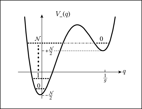
At $g=0$, the two wells become disjoint and two spectrum towers appear at around $q=0$ and $q=1/g$. For integer values of ${\cal N}$, the ${\cal N}$-th excited state is degenerate, with the lowest state in the other tower. This is the case when the ${\cal N}$-fold supersymmetry exists and it protects the degeneracy when the coupling constant $g$ is turned on. The lowest ${\cal N}$-states that do not have the corresponding states in the other spectrum are called “Isolated States”, which are free from Borel singularities due to the ${\cal N}$-fold supersymmetry, and in fact the perturbative series for the energy eigenvalues of these states have a finite convergence radius in the $g$-plane [2].

The Hamiltonian ${\bf H}_{\cal N}$ is not equal to the anticommutator $\frac{1}{2}\{Q_{\cal N}^{\dagger},Q_{\cal N}\}$ unless ${\cal N}=1$, which is the ordinary supersymmetric case. This is evident from the fact that $Q_{\cal N}$ contains ${\cal N}$-derivatives with respect to the coordinate $q$ and therefore $\frac{1}{2}\{Q_{\cal N}^{\dagger},Q_{\cal N}\}$ contains $2{\cal N}$-derivatives. The latter has, on the other hand, a ”family resemblance” to the Hamiltonian, and is thus called the “Mother Hamiltonian”;

$${\cal H}_{\cal N}\equiv\frac{1}{2}\{Q_{\cal N}^{\dagger},Q_{\cal N}\}=\left(\begin{array}[]{cc}\displaystyle\frac{1}{2}D^{\cal N}D^{\dagger\cal N}&0\\ 0&\displaystyle\frac{1}{2}D^{\dagger\cal N}D^{\cal N}\end{array}\right).$$ (19)

The following commutation relation is, of course, satisfied:

$$[{\cal H}_{\cal N},Q_{\cal N}]=[{\cal H}_{\cal N},Q_{\cal N}^{\dagger}]=0.$$ (20)

It was conjectured that this Mother Hamiltonian ${\cal H}_{\cal N}$ is a polynomial of the ordinary Hamiltonian ${\bf H}_{\cal N}$;

$${\cal H}_{\cal N}=\frac{1}{2}\det{\bf M}_{\cal N}({\bf H}_{\cal N}),$$ (21)

where ${\bf M}_{\cal N}$ is a ${\cal N}\times{\cal N}$ matrix obtained from the perturbative solution of the ${\cal N}$ isolated states [2]. The identity (21) was proven for ${\cal N}=1,2,3$ by hand, and for values up to ${\cal N}=10$ by the use of Mathematica.

3 A no-go theorem

As noted before the ${\cal N}$-fold supersymmetry for ${\cal N}=2,3,\cdots$ were found only for the particular $W(q)$ defined by Eq.(18), while the ${\cal N}=1$ ordinary supersymmetry holds for any arbitrary function $W(q)$. Therefore it is most natural to explore what other kinds of $W(q)$ allow ${\cal N}$-fold supersymmetry. Furthermore, for the quadratic $W(q)$ the supersymmetry is spontaneously broken. Therefore it is interesting to examine if ${\cal N}$-fold supersymmetry exists without spontaneous supersymmetry breaking.

It is possible to explore what kind of $W(q)$ is allowed under the supercharges (13), but with the following generalized Hamiltonian:

$$H_{\pm{\cal N}}=\frac{1}{2}p^{2}+\frac{1}{2}\left(W^{2}(q)\pm f_{\cal N}^{(\pm)}(q)\right).$$ (22)

The components of the desired commutation relation (17) are the following:

$$D^{\cal N}H_{-\cal N}=H_{+\cal N}D^{\cal N},$$ (23)

and its conjugate. In order to find the constraints for $W(q)$ and $f_{\cal N}^{(\pm)}(q)$ induced by the above relation, we will calculate the difference between the l.h.s. and the r.h.s. of the above:

$$2(D^{\cal N}H_{-\cal N}-H_{+\cal N}D^{\cal N})$$

$$\quad=D^{\cal N}(D^{2}+W^{\prime}+2iWD-f_{\cal N}^{(-)})-(D^{2}+W^{\prime}+2iWD+f_{\cal N}^{(+)})D^{\cal N}$$

$$\quad=D^{\cal N}W^{\prime}-W^{\prime}D^{\cal N}+2iD^{\cal N}WD-2iWD^{{\cal N}+1}-D^{\cal N}f_{\cal N}^{(-)}-f_{\cal N}^{(+)}D^{\cal N}$$ (24)

where we used a relation $p^{2}+W^{2}=D^{2}+W^{\prime}+2iWD$. Since

$$D=-i\,U^{-1}\partial\,U,\quad U=e^{\int W(q)dq}$$ (25)

where $\partial=\partial/\partial q$, we may transform all the $D$s to $\partial\,$s by the $U$-transformation;

$$i^{\cal N}U2(D^{\cal N}H_{-\cal N}-H_{+\cal N}D^{\cal N})U^{-1}$$

$$\qquad=\partial^{\cal N}W^{\prime}-W^{\prime}\partial^{\cal N}+2\partial^{\cal N}W\partial-2W\partial^{{\cal N}+1}-\partial^{\cal N}f_{\cal N}^{(-)}-f_{\cal N}^{(+)}\partial^{\cal N}$$ (26)

The next step is to move all the derivatives to the right and examine the coefficients of a given power of $\partial$. It is straightforward to show that the coefficients of $\partial^{{\cal N}+2}$ and $\partial^{{\cal N}+1}$ vanish identically. The $\partial^{{\cal N}}$ term and $\partial^{{\cal N}-1}$ term yields the following, respectively:

$$2{\cal N}W^{\prime}-f_{\cal N}^{(+)}-f_{\cal N}^{(-)}=0$$ (27)

$${\cal N}W^{\prime\prime}-f_{\cal N}^{(-)\prime}=0$$ (28)

These lead to;

$$f_{\cal N}^{(-)}={\cal N}W^{\prime}+C,\quad f_{\cal N}^{(+)}={\cal N}W^{\prime}-C,$$ (29)

where $C$ is an integration constant. This reproduces the original Hamiltonian (14) with a meaningless constant $C$ added. From the coefficient of $\partial^{{\cal N}-2}$ we find the following:

$$-\frac{1}{6}{\cal N}({\cal N}-1)({\cal N}+1)W^{\prime\prime\prime}=0.$$ (30)

The lower powers of $\partial$ have coefficients proportional to the derivatives of $W$ of order four or more. Therefore, we conclude that under the assumption of the form of the supercharges (13) and the Hamiltonian (22), the commutation relation (17) holds only for the following three cases: (1) ${\cal N}=0$, the trivial case with arbitrary $W(q)$, (2) ${\cal N}=\pm 1$, the ordinary supersymmetry with arbitrary $W(q)$, and (3) $W^{\prime\prime\prime}=0$, the quadratic $W(q)$ found previously.

This proves that as long as the supercharges are of the form (13), no new ${\cal N}$-fold supersymmetry is possible.

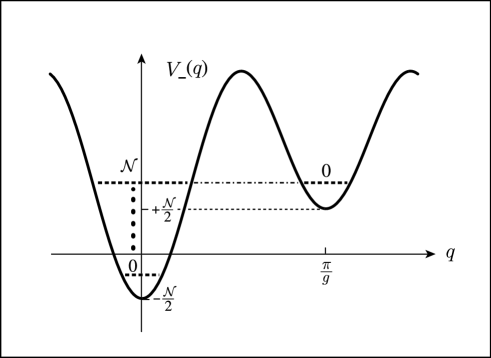
4 The periodic case

We will now examine the following case:

$$W(q)=\frac{1}{g}\sin(gq),$$ (31)

with periodicity $2\pi/g$. Ordinary supersymmetry is not broken since the region of $q$ is finite, unlike the quadratic case.

We define new ${\cal N}$-fold supercharges by the following:

$$Q_{\cal N}=\left(\begin{array}[]{cc}0&0\\ P_{\cal N}^{\dagger}&0\end{array}\right), \quad Q_{\cal N}^{\dagger}=\left(\begin{array}[]{cc}0&P_{\cal N}\\ 0&0\end{array}\right),$$ (36)

$$P_{\cal N}\equiv \prod_{k=-{\cal M}}^{\cal M}(D+kg),$$ (37)

where ${\cal N}=2{\cal M}+1$. Note that the above product is always in the range $-{\cal M},-{\cal M}+1,\cdots,{\cal M}-1,{\cal M}$ even for the half integer ${\cal M}$ (even ${\cal N}$). The supercharges (36) contain ${\cal N}$-derivatives, but are different from the form (13), and are free from the constraint of the no-go theorem proven in the previous section. The Hamiltonian is the same as in Eqs.(14) and (15). The potential of $H_{-\cal N}$ is illustrated in Fig.2.

Figure 2: The potential of $H_{-\cal N}$ for $W(q)=(1/g)\sin(gq)$ for $q\in[-\pi/(2g),3\pi/(2g)]$. The potential for $H_{+\cal N}$ is obtained by a reflection $q\rightarrow\pi/(2g)-q$. The energy levels are denoted by broken lines.

We first prove the commutation relation (17), whose components are;

$$P_{\cal N}H_{-\cal N}=H_{+\cal N}P_{\cal N},$$ (38)

and its conjugate. As in the previous section, we transform the both sides of the above identity by the $U$-transformation. The following is useful for this calculation:

$$UP_{\cal N}U^{-1} = \prod_{k=-{\cal M}}^{\cal M}(-i\partial+kg),$$ (39)

$$UH_{-\cal N}U^{-1} = -\frac{1}{2}\partial^{2}+\frac{e^{igq}}{2g}(-i\partial-{\cal M}g)-\frac{e^{-igq}}{2g}(-i\partial+{\cal M}g),$$ (40)

$$UH_{+\cal N}U^{-1} = -\frac{1}{2}\partial^{2}+\frac{e^{igq}}{2g}\left(-i\partial+({\cal M}+1)g\right)-\frac{e^{-igq}}{2g}\left(-i\partial-({\cal M}+1)g\right).$$ (41)

The l.h.s. of Eq.(38) is then calculated as follows:

$$UP_{\cal N}H_{-\cal N}U^{-1} = -\frac{1}{2}\partial^{2}P_{\cal N}+\frac{e^{igq}}{2g}\prod_{k=-{\cal M}}^{\cal M}\left(-i\partial+(k+1)g\right)(-i\partial-{\cal M}g)$$ (42)

$$-\frac{e^{-igq}}{2g}\prod_{k=-{\cal M}}^{\cal M}\left(-i\partial+(k-1)g\right)(-i\partial+{\cal M}g),$$

which is identical to $UH_{+\cal N}P_{\cal N}U^{-1}$. This completes the proof of (38).

There is an alternative, more complex but more direct, proof of the identity (38), which is similar to the proof of the quadratic case in Ref.[2]. We first note the following relation:

$$H_{+{\cal N}}D=DH_{+({\cal N}-2)}+\frac{g}{4}({\cal N}-1)\left[-e^{igq}+e^{-igq}\right].$$ (43)

Using this relation repeatedly, it is possible to show the following relation for any integer ${\cal N}^{\prime}(=2{\cal K}+1)$ and ${\cal N}(=2{\cal M}+1)$ by the mathematical induction for ${\cal N}^{\prime}$:

$$H_{+\cal N}P_{\cal N^{\prime}} = P_{\cal N^{\prime}}H_{+({\cal N}-2{\cal N^{\prime}})}+\frac{g}{4}{\cal N^{\prime}}({\cal N-N^{\prime}})P_{{\cal N^{\prime}}-2}\left[-(D-{\cal K}g)e^{igq}+(D+{\cal K}g)e^{-igq}\right].$$

This relation reproduces the desired commutation relation (38) for ${\cal N}^{\prime}={\cal N}$.

If we now turn to the isolated states and the Mother Hamiltonian next, we see that in the ordinary ${\cal N}$-fold supersymmetry, the algebra (23) guarantees that any solution $\Psi_{-\cal N}$ of the Shrödinger equation of the Hamiltonian $H_{-{\cal N}}$ is a solution of the Hamiltonian $H_{+{\cal N}}$ with the same eigenvalue, unless it is eliminated by $D^{\cal N}$;

$$D^{\cal N}\Psi_{-\cal N}=0.$$ (45)

This equation is satisfied by

$$\Psi_{-\cal N}=f(q)\,e^{-\int W(q)dq},$$ (46)

where $f(q)$ is a polynomial of order ${\cal N}-1$ or less. The solution (46) is not normalizable due to the $gq^{2}$-term in $W(q)$, but it is so at any finite order of the perturbation expansion in $g$. Thus the perturbative properties, especially the energy eigenvalues, of the isolated states are determined completely by the ${\cal N}$-fold supersymmetry. The fact that the solution (46) is not normalizable means that there are nonperturbative corrections on the isolated states and the ${\cal N}$-fold supersymmetry is spontaneously broken [2].

In the current case, we have

$$P_{\cal N}\Psi_{-\cal N}=0,$$ (47)

in place of (45), which is satisfied by $f(q)$ of the form of the truncated Fourier series;

$$f(q)=\sum_{k=-{\cal M}}^{\cal M}a_{k}\,e^{-ikgq}.$$ (48)

By substituting the above into the Shrödinger equation $H_{-\cal N}\Psi_{-\cal N}=E\Psi_{-\cal N}$ and using (40), we find the following set of equations for the coefficients ($a_{-\cal M},\cdots a_{\cal M}$):

$$(k+1+{\cal M})a_{k+1}+(2E-k^{2}g^{2})a_{k}-(k-1-{\cal M})a_{k-1}=0,$$ (49)

for $k=-{\cal M},\cdots{\cal M}$, where $a_{{\cal M}+1}$ and $a_{-({\cal M}+1)}$ should be understood to be zero. We rewrite the above to the matrix equation for the vector ${\bf a}_{\cal N}=(a_{-\cal M},\cdots,a_{\cal M})^{\rm T}$ as follows:

$${\bf M}_{\cal N}(E)\cdot{\bf a}_{\cal N}=0.$$ (50)

The energies of the isolated states are obtained from the following condition that nontrivial ${\bf a}_{\cal N}$ are allowed as solutions of the above;

$$\det{\bf M}_{\cal N}(E)=0.$$ (51)

It should be noted that unlike the quadratic case, the solutions of Eq.(51) are exact: Their wavefunctions are normalizable and therefore there are no nonperturbative corrections to the energy levels obtained from Eq.(51). Since Eq.(51) is a polynomial equation for $E$, its solutions have a finite convergence radius in $g$ and thus is Borel-summable. For example, at ${\cal N}=3$, Eq.(51) yields the following;

$$\det{\bf M}_{3}(E)=(2E-g^{2})(4(E^{2}-1)-2Eg^{2})=0,$$ (52)

whose solutions have infinite convergence radius. It is interesting to note that the exact energy of the first excited state is $E=g^{2}/2$, which is only the first order correction, which is analogous to the ABS anomaly. It should be noted that these solutions for the isolated states come with specific boundary conditions; periodic for odd ${\cal N}$ and anti-periodic for even ${\cal N}$. No exact solutions with other twisted boundary conditions has been found so far.

We conjecture that the Mother Hamiltonian ${\cal H}_{\cal N}$ defined by

$${\cal H}_{\cal N}\equiv\frac{1}{2}\{Q_{\cal N}^{\dagger},Q_{\cal N}\},$$ (53)

with the supercharges (36) is again given by the following polynomial of the usual Hamiltonian;

$${\cal H}_{\cal N}=\frac{1}{2}\det{\bf M}_{\cal N}({\bf H}_{\cal N}).$$ (54)

We have proven the above identity directly for ${\cal N}=3$ by the use of Mathematica.

We have found some further extensions of the ${\cal N}$-fold supersymmetry are possible, including cubic and exponential $W(q)$s. This and further general discussions will be published in the near future.

Acknowledgment

The authors would like to thank Dr. Hisashi Kikuchi (Ohu University, Japan) for discussions and Dr. John Constable (Magdalene College, U.K.) for reading the manuscript. H. Aoyama’s work was supported in part by the Grant-in-Aid for Scientific Research No.10640259. T. Tanaka’s work was supported in part by a JSPS research fellowship.

References

- [1] E. Witten, Nucl. Phys. B202 (1982) 253.
- [2] H. Aoyama, H. Kikuchi, I. Okouchi, M. Sato, and S. Wada, Nucl. Phys. B553 (1999) 644.
- [3] D. J. Rowe and A. Ryman, J. Math. Phys. 23 (1982) 732.
- [4] I. I. Balitsky and A. V. Yung, Phys. Lett. B168 (1986) 13.
- [5] P. G. Silvetrov, Sov. J. Nucl. Phys. 51 (1990) 1121.
- [6] H. Aoyama and H. Kikuchi, Nucl. Phys. B369 (1992) 219.
- [7] H. Aoyama and S. Wada, Phys. Lett. B349 (1995) 279.
- [8] T. Harano and M. Sato, hep-ph/9703457.
- [9] H. Aoyama, H. Kikuchi, T. Harano, M. Sato, and S. Wada, Phys. Rev. Lett. 79 (1997) 4052.
- [10] H. Aoyama, H. Kikuchi, T. Harano, I. Okouchi, M. Sato, S. Wada, Prog. Theor. Phys. Supplement 127 (1997) 1.
- [11] H. Aoyama, H. Kikuchi, I. Okouchi, M. Sato, and S. Wada, Phys. Lett. B424 (1998) 93.
- [12] E. B. Bogomolny, Phys. Lett. B91 (1980) 431.
- [13] E. Witten, Nucl. Phys. B188 (1981) 513.
- [14] P. Solomonson and J. W. Van Holten, Nucl. Phys. B196 (1982) 509.
- [15] F. Cooper, A. Khare, and U. Sukhatme, Phys. Rep. 251 (1995) 267.