Entanglement of coherent states and decoherence

Abstract

A possibility to produce entangled superpositions of strong coherent states is discussed. A recent proposal by Howell and Yazell [Phys. Rev. A 62, 012102 (2000) ] of a device which entangles two strong coherent coherent states is critically examined. A serious flaw in their design is found. New modified scheme is proposed and it is shown that it really can generate non-classical states that can violate Bell inequality. Moreover, a profound analysis of the effect of losses and decoherence on the degree of entanglement is accomplished. It reveals the high sensitivity of the device to any disturbances and the fragility of generated states.

I Introduction

Quite recently an interesting idea has been proposed [1] how to entangle two strong coherent fields and generate a four-mode Schrödinger cat-like state utilizing quantum non-demolition (QND) measurement. The idea has been inspired by recent works on a similar subject [2]. However, the authors made a serious mistake in their reasoning, which renders their experimental scheme unworkable. Before we show how to modify the scheme in order to get the desired effect we shall briefly discuss the original experimental arrangement.

The original scheme for entangling “macroscopic” fields is that outlined in Fig. 1 without beam splitter BS and detectors D₁ and D₂. The idea goes as follows. First, a non-separable single photon state

$$(|1\rangle_{12}|0\rangle_{13}+i|0\rangle_{12}|1\rangle_{13})/\sqrt{2}$$ (1)

is produced using the single-photon source SPS and a 50:50 beam splitter. In the next step an attempt is made to transfer the which-path uncertainty of the photon into the entanglement of strong coherent fields generated by the coherent sources CS by means of non-demolition measurements of the number of photons in modes $12$ and $13$. The QND measuring devices operate by the cross-Kerr interaction described by the Hamiltonian

$$H_{\rm QND}=\hbar\pi(\hat{n}_{12}\hat{n}_{23}+\hat{n}_{13}\hat{n}_{33}),$$ (2)

where $\hat{n}$ are photon number operators of the corresponding modes. The strengths of the interactions (2) are carefully chosen so as to yield the accumulated phase shift of $\pi$ in modes $23$ or $33$ provided a single photon is present in modes $12$ or $13$, respectively. This means that the presence of a single photon, for instance, in $12$ mode will cause the outputs of $24$ and $25$ modes to be switched completely. This switching lies in the heart of the quantum entangling device which according to Howell and Yeazell [1] should generate four-mode “macroscopic” entangled state

$$|\Phi\rangle=N_{+}(|\phi_{1}\rangle+|\phi_{2}\rangle),$$ (3)

where

$$|\phi_{1}\rangle = |\alpha_{2}\rangle_{24}|0\rangle_{25}|0\rangle_{34}|\alpha_{3}\rangle_{35}$$ (4)

$$|\phi_{2}\rangle = |0\rangle_{24}|\alpha_{2}\rangle_{25}|\alpha_{3}\rangle_{34}|0\rangle_{35}.$$ (5)

Here $\alpha_{2}$ and $\alpha_{3}$ are complex amplitudes proportional to the amplitudes of the coherent fields fed into the inputs $21$ and $31$, respectively, and $N_{+}$ is a normalization factor [3]. However, the four-mode output state was not calculated explicitly in [1]. The authors rather guessed at the four-mode state from the results of a few thought experiments with the output light. The authors’ claim that the observed correlations are of a purely quantum nature and could not be explained classically is in error, though. It could be easily demonstrated that the correlations discussed in [1] can be explained by the following mixed four-mode state,

$$\rho=\frac{1}{2}(|\phi_{1}\rangle\langle\phi_{1}|+|\phi_{2}\rangle\langle\phi_{2}|),$$ (6)

that is by the “classical” statistical mixture, which is usually referred to as a separable mixture or a state containing only classical correlations. It is not difficult to see that it is the mixed (classical) state (6) rather than cat state (3) what is produced by the original Howell and Yeazell’s apparatus. Working in the Schrödinger picture, the output six-mode state can straightforwardly be calculated as follows

$$|\Phi_{\rm all}\rangle=\frac{1}{\sqrt{2}}\left(|\phi_{1}\rangle|0\rangle_{12}|1\rangle_{13}+|\phi_{2}\rangle|1\rangle_{12}|0\rangle_{13}\right).$$ (7)

It is the photon leaving the apparatus in modes $12$, $13$ and carrying which-way information what destroys the entanglement among the remaining four modes. Mathematically, the output state of four modes $24$, $25$, $34$, $35$ is obtained by tracing the density matrix $|\Phi_{\rm all}\rangle\langle\Phi_{\rm all}|$ over the two modes; we end up with the mixed state (6). This somehow slipped attention of the authors in [1].

II QND entangling device

Having identified the catch in the original scheme one can try to work around it. The key point is to erase the which-way information that resides in $12$ and $13$ two-mode field when the interaction is over. To accomplish this we propose to superimpose these modes at a 50:50 beam splitter BS as shown in Fig. 1. Two single photon detectors D₁ and D₂ are attached to the outputs of beam splitter BS. After mixing the $12$ and $13$ beams at the beam splitter the state of the six-mode field reads

$$|\Phi_{\rm all}\rangle = \frac{1}{2}\left[-(|\phi_{1}\rangle-|\phi_{2}\rangle)|0\rangle_{14}|1\rangle_{15}\right.$$ (9)

$$+i\left.(|\phi_{1}\rangle+|\phi_{2}\rangle)|1\rangle_{14}|0\rangle_{15}\right].$$

Now, depending on the result of the single-photon detection, the four-mode state of interest becomes

$$|\Phi_{1}\rangle=N_{+}(|\phi_{1}\rangle+|\phi_{2}\rangle),$$ (10)

if D₁ detector fires, or

$$|\Phi_{2}\rangle=N_{-}(|\phi_{1}\rangle-|\phi_{2}\rangle),$$ (11)

if D₂ does. $N_{-}$ is a normalization factor [3]. We remind that for $|\alpha_{2}|,|\alpha_{3}|\gg 1$ the four-mode states $|\phi_{1}\rangle$ and $|\phi_{2}\rangle$ are well separated “macroscopic” states. Hence we arrived at the sought after effect. In fact two kinds of phase shifted Schrödinger cat-like states can be generated using the scheme depicted in Fig. 1. Now a perfect source of the “macroscopic” entangled field can be realized using a gate triggered by the D₁ and D₂ detectors so that only one of the states (10) and (11) is allowed to go through.

Here a comment seems to be in order. Had the information gained by means of detectors D₁ and D₂ been not used for post-selecting the state of the remaining four modes, we would have had the same four-mode output field as Howell and Yeazell had. Ignoring the result of the single-photon detection amounts to taking the weighted average of the states $|\Phi_{1}\rangle$ and $|\Phi_{2}\rangle$. It is not difficult to see that the averaging bring us back to the mixed state (6). This is consistent with quantum theory because no tampering with modes $14$, $15$ can influence the results of experiments performed on the remaining (possibly space-like separated) beams. We should also mention that the idea used in this report to correct the original faulty scheme is in fact an implementation of the well-known and much discussed quantum eraser [4].

Let us close this section observing that actually the amended setup (Fig. 1) is unnecessarily too complicated; it contains redundant parts. One can easily do with just one QND device. Let us remove the rightmost Mach-Zehnder (MZ) interferometer and its QND device from the setup. The output state will change to $(|0\rangle_{34}|\alpha_{3}\rangle_{35}+|\alpha_{3}\rangle_{34}|0\rangle_{35})/\sqrt{2}$, supposing that a click at detector $D_{1}$ have been registered. After using two additional beam splitters in $34$ and $35$ paths and re-labeling the output modes, the four-mode entangled state equivalent to (3) is obtained again.

III Entanglement and nonlocality

Before discussing decoherence which could be serious obstacle in the way of realizing the “macroscopic” entangler in laboratory, let us discuss briefly some interesting properties of the “cat” state (3). First of all one may ask, to which extend the state (3) is entangled. We will adopt mutual information as a convenient measure of entanglement [5]. It is defined by the difference between the sum of von Neumann entropies $S_{1}$ and $S_{2}$ of subsystems $1$ and $2$ and the von Neumann entropy of the composite system $S$:

$$I=S_{1}+S_{2}-S.$$ (12)

Here subsystem $1$ consists of modes $24$ and $25$; subsystem $2$ consists of modes $34$ and $35$. Mutual information (12) is zero if the subsystems 1 and 2 are uncorrelated ($\rho$=$\rho_{1}\otimes\rho_{2}$). Its maximum value still explainable by classical correlations is $I=S$ [6].

For simplicity we will consider symmetric inputs $\alpha_{2}=\alpha_{3}=\alpha$. Although explicit calculation of mutual information $I$ for general input coherent state is tedious, it is not difficult to ascertain its lower and upper band. For very small input amplitude $|\alpha|\ll 1$ state (3) becomes nearly a product state, hence its mutual information goes to zero. Maximum is attained for very large $|\alpha|$ – such that the two components in (3) become almost orthogonal states. Then one obtains

$$I_{\rm max}=2\ln 2.$$ (13)

An issue closely related to entanglement is question whether particular entangled states can violate local realism [7]. Noticing that for $\alpha\gg 1$ two-dimensional subspace spanned by vectors $|\alpha,0\rangle_{1}\equiv|\alpha\rangle_{24}|0\rangle_{25}$ and $|0,\alpha\rangle_{1}$, living in Hilbert space of the first system is isomorphic to spin-half particle space (similarly for system $2$), one can define unitary operations

$$|\alpha,0\rangle_{1} \rightarrow M_{+}(\cos\theta\,|\alpha,0\rangle_{1}+\sin\theta\,|0,\alpha\rangle_{1})$$ (14)

$$|0,\alpha\rangle_{1} \rightarrow M_{-}(-\sin\theta\,|\alpha,0\rangle_{1}+\cos\theta\,|0,\alpha\rangle_{1})$$ (15)

(similarly for system $2$), which are in some sense analogous to spin rotations. $M_{\pm}$ are normalization factors [3]. Bell-type experiment then consists of two “rotations” according to the recipe (14) performed by two possibly space-like separated observers, followed by realistic yes–no detection performed on each mode. Each such detection has only two possible outcomes (detector either fire or it does not). Let us assign them values $z_{i}$=0 if the detector (in mode $i$) is quiet and $z_{i}$=1 if it clicks. Then the results $X$ and $Y$ of the local two-mode measurements (including “rotations”) performed by the first and second observer, respectively, can be expressed as

$$X(\theta) = z_{24}(\theta)-z_{25}(\theta),$$ (16)

$$Y(\theta) = z_{34}(\theta)-z_{35}(\theta).$$ (17)

After the experiment is repeated many times and the two observers compare their notes, the following quantity can be estimated

$$B=|C(\theta_{1},\theta_{2})+C(\theta_{1},\theta_{2}^{\prime})+C(\theta_{1}^{\prime},\theta_{2})-C(\theta_{1}^{\prime},\theta_{2}^{\prime})|,$$ (18)

where correlation function

$$C(\theta_{1},\theta_{2})\equiv\sum_{j,k}X_{j}Y_{k}\,p(X_{j},Y_{k}|\theta_{1},\theta_{2}).$$

As with the two spin-half particles the use of (3) and (14) in (18) gives $B_{\max}=2\sqrt{2}$, for optimum set of angles. This exceeds local realistic limit $B^{\rm cl}_{\rm max}=2$ [8]. Thus from the point of view of entanglement and local realism the four-mode state (3) is equivalent to the maximally entangled state of two spin-half particles. This is, of course, consequence of the fact that the “cat” state (3) is nothing else than representation of the maximally entangled spin state in a larger space – in the space of four harmonic oscillators.

While spin of e.g. neutron can be easily rotated in magnetic field, it is very difficult to realize the corresponding unitary transformation (14). Notice that although the device in Fig. 1 does a similar job (it creates superpositions from the input product states of a similar sort) its action is not unitary due to the postselection involved. This would represent a loophole in the test of local realism when used in place of the unitary transformation (14).

IV Decoherence

So far we assumed that the entangling device was ideal. This seems natural if fundamental aspects of thought device are discussed. If one, however, seriously thought of experimental implementation of the entangling device in Fig. 1, such assumption would clearly be foolish, and various imperfections and unavoidable losses would have to be considered.

The entangling device can be divided into two parts, the one-photon MZ interferometer and coherent-state MZ interferometers, with grossly different sensitivity to imperfections and losses. This can be illustrated on the simple case of losses modeled e.g. by the presence of an auxiliary beam splitter in the paths of modes 23, 33, and 12. In the latter case one can always balance the one-photon interferometer by introducing the same amount of losses in mode 13, recovering the ideal output state (3) at the expense of decreasing generation rate [9]. In such a case, if the photon is detected behind the interferometer, no information on its path is available and entanglement in the whole state is kept (if the losses were not balanced, one path would be more probable). In contrast to it, a similar compensation of losses in the coherent-state interferometers cannot help to save the entanglement. It is not difficult to see why. The fractions of the strong coherent beams reflected out of the coherent-state interferometer always carry a good deal of which-way information about the photon in the one-photon MZ interferometer, that can be extracted, e.g., by means of the phase measurement performed on them. Needles to say, in the limit of large $\alpha$, when the phase of the reflected beam becomes sharply defined, the reflected beams carry perfect which-way information about the photon propagating through the one-photon interferometer; this degrades the output state (3) to the mixed state (6). Another likely causes of the loss of entanglement of the output state are decoherence effects due to entangling the degrees of freedom of the quantum system with environment. First, let us discuss the decoherence in the one-photon Mach-Zehnder interferometer consisting of modes $12$ and $13$. We will assume the following simple (but rather general) model of decoherence,

$$|0\rangle_{12}|g\rangle_{\rm env} \rightarrow |0\rangle_{12}|e_{1}\rangle_{\rm env},$$ (19)

$$|1\rangle_{12}|g\rangle_{\rm env} \rightarrow |1\rangle_{12}|e_{2}\rangle_{\rm env},$$ (20)

where $|g\rangle_{\rm env}$, $|e_{1}\rangle_{\rm env}$ and $|e_{2}\rangle_{\rm env}$ are three possibly nonorthogonal states of environment. Denoting $a$ the overlap $a=|\langle e_{1}|e_{2}\rangle|$, the mutual information of the output state for large $|\alpha|$ reads,

$$I \approx 2\ln 2+\frac{1+a}{2}\ln\left(\frac{1+a}{2}\right)$$ (22)

$$+\frac{1-a}{2}\ln\left(\frac{1-a}{2}\right),\quad|\alpha|\gg 1.$$

Similarly, the maximum of the Bell correlation function is reduced to

$$B_{\max}\approx\sqrt{2}(1+a),\quad|\alpha|\gg 1.$$ (23)

For exact formulas see Appendix.

Note that $a^{2}$ equals the Ivanovics-Dieks-Peres lower bound [10] on the probability of the occurrence of an inconclusive result for error-free discrimination between the two non-orthogonal states of environment and therefore also between the states $|0\rangle_{12}$ and $|1\rangle_{12}$. Hence, one can say that as the amount of principally accessible which-way information about the photon in the one-photon MZ interferometer increases, the entanglement and non-classical character of the output state of the entangling machine become gradually destroyed. Eqs. (22) and (23) should be compared with the corresponding formulas for entangling machine with (balanced) losses present in the coherent state MZ interferometers. We will model the losses by placing four auxiliary beam splitters with the same reflectivity $R$ into $22$, $23$, $32$ and $33$ paths. The resulting asymptotic entanglement and maximum of the Bell correlation function are

$$I \approx 2\ln 2+\frac{1+e^{-2R|\alpha|^{2}}}{2}\ln\left[\frac{1+\exp(-2R|\alpha|^{2})}{2}\right]$$ (24)

$$+ \frac{1-e^{-2R|\alpha|^{2}}}{2}\ln\left[\frac{1-\exp(-2R|\alpha|^{2})}{2}\right],\quad|\alpha|\gg 1,$$ (25)

and

$$B_{\max}\approx\sqrt{2}\left(1+e^{-2R|\alpha|^{2}}\right),\quad|\alpha|\gg 1.$$ (26)

Notice that Eqs. (24) and (26) can be obtained from Eqs. (22) and (23) simply by substitution

$$a^{2}\rightarrow e^{-4R|\alpha|^{2}}.$$ (27)

This can again be interpreted in terms of available which-way information. Now, the which-way information is gained by discriminating between (non-orthogonal) states $|\alpha\sqrt{R/2}\rangle$ and $|-\alpha\sqrt{R/2}\rangle$ of the beams reflected out of paths $23$ and $33$. The optimum error-free discrimination is done by mixing the beams with the reference coherent beams $|i\alpha\sqrt{R/2}\alpha\rangle$ at two mixing beam splitters [11]. The probability of the inconclusive result: “no photons detected after the mixing at both outputs”, is $P_{\rm inconcl.}=\exp(-2R|\alpha|^{2})$ in either case. The path of the photon is revealed by getting at least one conclusive result out of the two ideal error-free measurements in the right and left part of the entangling apparatus. The probability of the unfortunate event of getting two inconclusive results is $P^{\rm total}_{\rm inconcl.}=P_{\rm inconcl.}^{2}=\exp(-4R|\alpha|^{2})$, which is just the right hand side of Eq. (27). This suggests that the loss of entanglement and non-locality caused by both effects, the decoherence in the one-photon interferometer and losses or decoherence in the coherent-state interferometers, have common information-theoretical origin.

Although Eqs. (24)–(26) and (22)–(23) have the same functional dependence on the amount of available which-way information, their implications for the feasibility of the generation of the “macroscopic-cat” state (3) dramatically differ. The decoherence in the one-photon MZ interferometer is not a key limiting factor for engineering such superpositions for Eqs. (22) and (23) does not depend on the intensity of the input coherent state $|\alpha|^{2}$. In contrast to this, the relative amount of losses in the coherent-state interferometers which can be tolerated, exponentially decreases with increasing input intensity, see Eqs. (24) and (26). This precludes the entangling of arbitrarily separated coherent states.

Forgetting about macroscopical separability, the presented device can still be a useful tool for generating interesting non-classical states. This is illustrated in Fig. 2. The degree of entanglement $I$ in the presence of losses is shown in Fig. 2(a). Notice that for large $|\alpha|$ the entanglement of the output state is extremely sensitive to the presence of losses. With increasing amount of losses the output state becomes mixed state and the correlations between output modes become explainable classically (large flat area). For still larger $|\alpha|$, all output modes get depleted and $I$ drops to zero. Two scales of sensitivity to disturbances are involved; one corresponds to the vanishing of nondiagonal elements of density matrix, the other corresponds to the loss of orthogonality between correlated output states. It can be seen that generation of output states having non-classical correlations is possible for not very large input intensities.

Similar discussion holds also for the maximum attainable value of Bell correlation function $B_{\rm max}$, see Fig. 2(b). Here part of the graph lying above the local-realistic limit $B=2$ has been cut off. Resulting upper small flat area adjacent to plane $R=0$ indicates the range of parameters for which the generation of nonclassical states is possible. For realistic experimental setups one again has constraint on the maximum allowed input intensities.

It follows that experimental generation of nonclassical states using the proposed device is possible for not very large intensities $|\alpha|^{2}$. Such states are interesting from the point of view of possible interesting experiments on quantum nonlocality, or experiments utilizing quantum entanglement, but they are far from being entangled “macroscopic” states.

V Conclusion

We have shown that the “entangling” apparatus proposed in Ref. [1] could never produce entangled pairs of coherent states. We have designed a device that can do it. This device also uses Kerr nonlinear medium which helps to extend the one-photon non-separable superposition to the four-mode entangled superposition of strong coherent fields. The new important point is a postselection based on interferometric measurement on the one-photon subsystem. This erases which-way information that had prevented the creation of desired entangled state. We have proved that the states prepared by our prescription can violate Bell-like inequalities. We have also studied to which extend loses and decoherence can degrade the produced state. This is important with respect to potential experimental realization. Unfortunately, the preparation procedure is very sensitive to decoherence and especially to losses in the strong-field interferometers. However, some set of realistic values in parameter space still exists for which entropy of states exceeds classical level and even Bell inequality can be violated.

A Some exact formulae

Explicit formulae for mutual information (12) and Bell-factor (18) of the system in states (10) ($+$) and (11) ($-$) are as follows

$$I_{\pm}=p_{1\pm}\ln p_{1\pm}+p_{2\pm}\ln p_{2\pm}-2(p^{r}_{1\pm}\ln p^{r}_{1\pm}+p^{r}_{2\pm}\ln p^{r}_{2\pm}),$$ (A1)

$$B_{\pm}=|C_{\pm}(\theta_{I},\theta_{II})+C_{\pm}(\theta_{I},\theta^{{}^{\prime}}_{II})+$$ (A2)

$$+C_{\pm}(\theta^{{}^{\prime}}_{I},\theta_{II})-C_{\pm}(\theta^{{}^{\prime}}_{I},\theta^{{}^{\prime}}_{II})|.$$ (A3)

Here

$$p_{1\pm} = \frac{(1\pm d)(1+\mu^{2})}{2(1\pm\mu^{2}d)},$$ (A4)

$$p_{2\pm} = \frac{(1\mp d)(1-\mu^{2})}{2(1\pm\mu^{2}d)},$$ (A5)

$$p^{r}_{1\pm} = \frac{(1\pm\mu d)(1+\mu)}{2(1\pm\mu d)},$$ (A6)

$$p^{r}_{2\pm} = \frac{(1\mp\mu d)(1-\mu)}{2(1\pm\mu d)},$$ (A7)

$$C_{\pm}(\theta_{I},\theta_{II}) = N_{\pm}^{2}\left((N_{1}+N_{2})\cos(2\theta_{I})\cos(2\theta_{II})\mp\right.$$ (A9)

$$\left.\mp 2dN_{3}\sin(2\theta_{I})\sin(2\theta_{II})\right),$$

and

$$N_{1} = \frac{1}{(1+\mu\sin(2\theta_{I}))(1-\mu\sin(2\theta_{II}))},$$ (A10)

$$N_{2} = \frac{1}{(1-\mu\sin(2\theta_{I}))(1+\mu\sin(2\theta_{II}))},$$ (A11)

$$N_{3} = \frac{1}{\sqrt{(1-\mu\sin^{2}(2\theta_{I}))(1-\mu\sin^{2}(2\theta_{II}))}}.$$ (A12)

Factor $\mu$ accounts for various disturbances. In the case of decoherence in the one-photon interferometer it reads

$$\mu=\exp(-|\alpha|^{2}),\hskip 14.22636ptd=\sqrt{1-|\langle e_{1}|e_{2}\rangle|^{2}}.$$ (A13)

In the case of balanced losses modeled by beam splitters present in the coherent-state interferometers one has

$$\mu=\exp(-T|\alpha|^{2}),\hskip 14.22636ptd=\exp(-2R|\alpha|^{2}).$$ (A14)

The maximum of $|B_{-}|$ occurs for angles

$$\theta_{I}=0,\theta^{{}^{\prime}}_{I}=\frac{\pi}{4},\theta_{II}=\frac{\pi}{8},\theta^{{}^{\prime}}_{II}=-\frac{\pi}{8}.$$ (A15)

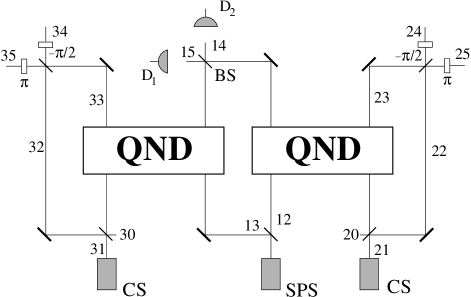
FIG. 1.: Entangling apparatus. QND – quantum non-demolition measuring devices; CS – coherent state sources; SPS – single-photon source; BS – beam splitter; D₁, D₂ – single-photon detectors.

FIG. 2.: Mutual information $I_{-}$ (a) and the maximum value of Bell correlation function $(B_{-})_{\rm max}$ (b) are shown for different input mean numbers of photons $\langle n\rangle\equiv|\alpha|^{2}$ and reflectivities $R$ of the beam splitters simulating losses.

REFERENCES

- [1] J.C. Howell and J.A.Yeazell, Phys. Rev. A 62, 012102 (2000).
- [2] B. C. Sanders, and G. J. Milburn, Phys. Rev. A 39, 694 (1989); B. C. Sanders, Phys. Rev. A 45, 6811 (1992); 46, 2966 (1992); B. Wielinga and B. C. Sanders, J. Mod. Opt. 40, 192 (1993); A. Mann, B. C. Sanders, and W. J. Munro, Phys. Rev. A 51, 989 (1995); B. C. Sanders, K. S. Lee, M. S. Kim, Phys. Rev. A 52, 735 (1995); D. A. Rice, and B. C. Sanders, Quantum. Semiclass. Opt. 10, L41 (1998); B. C. Sanders, and D. A. Rice, Opt. Quantum Electron. 31, 525 (1999); B. C. Sanders, and D. A. Rice, Phys. Rev. A 61, 013805 (2000); D. A. Rice, G. Jaeger, and B. C. Sanders, Phys. Rev. A 62, 012101 (2000);
- [3] ; .
- [4] M. Hillery and M. O. Scully, in Quantum Optics, Experimental Gravitation, and Measurement Theory, eds. P. Meystre and M. O. Scully (Plenum, New York, 1983), p. 65; M. O. Scully, B. G. Englert, and H. Walther, Nature 351, 111 (1991); P. G. Kwiat, A. M. Steinberg, and R. Y. Chiao, Phys. Rev. A 45, 7729 (1992); P. G. Kwiat, M. Aerphraim, A. M. Steinberg, and R. Y. Chiao, Phys. Rev. A 49, 61 (1994).
- [5] S.M.Barnett and S.J.D.Phoenix, Phys. Rev. A 40, 2404 (1989).
- [6] The diagonal representation of the density matrix of two correlated subsystems displaying maximum classically allowed correlations is of the form . Then one gets .
- [7] A. Einstein, B. Podolsky, N. Rosen, Phys. Rev. 47, 777 (1935); D. Bohm, Phys. Rev. 85, 166 (1952); N. Bohr, Nature 136, 65 (1935).
- [8] J. S. Bell, Physics 1, 195 (1964); J. F. Clauser, M. A. Horne, A. Shimony, R. A. Holt, Phys. Rev. Lett. 23, 880 (1969).
- [9] M. Hendrych, M. Dušek, O. Haderka, Acta Physica Slovaka 46, 393 (1996).
- [10] I.D. Ivanovic, Phys. Lett. A 123, 257 (1987); D. Dieks, Phys. Lett. A 126, 303 (1998); A. Peres, Phys. Lett. A 128, 19 (1988).
- [11] B. Huttner, N. Imoto, N. Gisin, and T. Mor, Phys. Rev. A 51, 1863 (1995); L.S. Phillips, S.M.Barnett, and D.T. Pegg, Phys. Rev. A 58, 3259 (1998).