Semiclassical description of Stern-Gerlach experiments

Abstract

The motion of neutral particles with magnetic moments in an inhomogeneous magnetic field is described in a semi-classical framework. The concept of Coherent Internal States is used in the formulation of the semiclassical approximation from the full quantum mechanical expression. The classical trajectories are defined only for certain spin states, that satisfy the conditions for being Coherent Internal States. The reliability of Stern-Gerlach experiments to measure spin projections is assessed in this framework.

PACS numbers: 03.65.Sq, 03.65.Bz, 03.65.Nk, 24.10.-i, 24.70+s.

Keywords: Quantum Scattering Theory, Semiclassical Approximation, Spin, Magnetic field, Path integral methods, Quantum measurement.

I Introduction

The Stern-Gerlach experiment consists in taking a beam of particles that have a neutral electric charge, but a finite magnetic moment, and making them to go through an inhomogeneous magnetic field. The observed result is that the particles deflect differently depending on the spin projection along the magnetic field. So, by measuring the deflection, one can infer the value of the spin projection of the particles along the direction of the magnetic field. The Stern-Gerlach experiment is the archetype of the measurement of a quantum mechanical property. Thus, it is always discussed even in the most basic textbooks of quantum mechanics [1]. The explanation that it is usually done for the Stern-Gerlach experiment is of a semiclassical nature. The motion of the particles is approximated by classical trajectories. In the following, we will present a brief account of the description of the Stern-Gerlach experiment, as it is usually done in textbooks.

One starts with a beam of particles, in a certain spin state, moving initially along a straight line. For the following discussion, we will take the y-axis along the direction of the motion of the particles. The center of the beam corresponds to the coordinates $x=0,z=0$. The beam enters in a Stern-Gerlach magnet. Usually, the Stern-Gerlach magnets produce magnetic fields that are independent of y and that do not have components in the y-direction (neglecting border effects). The z-axis is chosen along the direction of the magnetic field at the center of the beam. So,

$$\vec{B}(\vec{r})=B_{z}(x,z)\hat{u}_{z}+B_{x}(x,z)\hat{u}_{x}$$ (1)

where $B_{x}(0,0)=0$. The geometry of the Stern-Gerlach magnet is such that $B_{z}(x,z)$ varies with $z$, but is mostly independent of $x$. Thus, a force appears in the z-direction which is proportional to $dB_{z}/dz\mu_{z}$. However, as the divergence of the magnetic field has to vanish, then $dB_{z}/dz=-dB_{x}/dx$, and so if the $B_{z}$ varies with $z$, then $B_{x}$ must vary with $x$. Thus, if we only retain terms linear in $x$ and $z$, we get

$$\vec{B}(\vec{r})=(B_{0}-B_{1}z)\hat{u}_{z}+xB_{1}\hat{u}_{x}$$ (2)

The magnetic field interacts with the magnetic moment of the particle $\mu$, giving rise to an interaction energy given by

$$E_{B}(\vec{r})=-\vec{B}(\vec{r})\cdot\vec{\mu}$$ (3)

This interaction energy depends on the distance. Thus, a force is generated which is given by

$$\vec{F}=-\vec{\nabla}E_{B}(\vec{r})=\vec{\nabla}B_{z}(x,z)\mu_{z}+\vec{\nabla}B_{x}(x,z)\mu_{x}$$ (4)

Thus, a force in the x-direction also appears which would be proportional to $dB_{x}/dx\mu_{x}$.

¿From the expression (4), the force acting on a particle with a certain spin state can be calculated. If we consider the scattering of particles which have a given spin projection $m$ along the z-axis, they will suffer a force that will be calculated as the expectation value in the z-direction which is proportional to the spin projection. The second term in (4) will not contribute because the matrix element $<m|\mu_{x}|m>$ vanishes. This result is well known, and it is in agreement with experiment. However, we can consider the case of the scattering of particles with spin projection $m^{\prime}$ along the x-axis. If we calculate the expectation value of $\vec{F}$ in (4), we obtain a force in the x-direction, while the force in the z-direction vanishes. This implies a deflection of the trajectory in the x-direction, that does not happen in the experiment. As any student of quantum mechanics should know, the trajectory is split in $2I+1$ trajectories, each one of which is deflected in the z-direction by a different amount.

In most of the basic textbooks of quantum-mechanics, the term proportional to $\mu_{x}$ in (4) is simply ignored [1]. Other more recent books, such as [2] and [3], only consider the spatial variation of the component $B_{z}$ of the magnetic field, but they neglect the variation of $B_{x}$. The classic book of quantum mechanics by Messiah [4] argues that $\mu_{z}$ is basically constant, while $\mu_{x}$ oscillates around zero. So, in the average of the force over many oscillations this term would cancel. This argument, although plausible, is hardly a firm ground on which to describe the general motion of particles in inhomogeneous magnetic fields. The opinion of the authors is that the Stern-Gerlach experiment still requires a satisfactory description in semiclassical terms.

In this paper we propose a semiclassical explanation to the Stern-Gerlach experiment. It relies on the concept of Coherent Internal States (CIS), that we introduced in a previous paper [5]. The conclusion of that paper was that when one analyzes the scattering of a particle with internal degrees of freedom, such as the spin, a single trajectory is a meaningful approximation for the quantum mechanical scattering wave function only for a certain set of internal states, which we called Coherent Internal States (CIS). Thus, if the scattered particle has an internal state that coincides initially with one of the CIS, then its scattering wavefunction can be approximated by a single trajectory. If not, the internal state should be expanded in terms of the CIS, and then the scattering wavefunction can be approximated by a combination of classical trajectories, one for each CIS.

In the case of Stern-Gerlach experiments, we demonstrate in section 2 that the CIS correspond to states with definite projection along the direction of the magnetic field. This direction, called $z^{\prime}$, may vary depending on the position of the particle, because the magnetic field is not homogeneous. So, it does not coincide with the laboratory fixed $z$-axis defining the direction of the magnetic field at the centre of the beam. In section 3 we use the path integral formalism to describe the trajectories of the CIS, and we find that they deflect on the $z^{\prime}$ direction. Considering that the average of $z^{\prime}$ corresponds to $z$, that explains the observed fact that the trajectories split in the z-direction, and not in the x-direction, as (4) could suggest. In section 4 we describe the scattering of a beam of particles with a finite size in a Stern-Gerlach magnet. As the axes $z^{\prime}$ and $z$ do not coincide, the deflection of the trajectory is not always consistent with the spin projection along the $z$ axis. So, a Stern-Gerlach magnet, understood as a measurement apparatus to find the spin projection along the $z$ axis, has a certain probability of giving a wrong result, which can be evaluated in our formalism. Section 5 is for the summary and conclusions.

II Coherent Internal States for a particle moving in an inhomogeneous magnetic field

It was shown in [5] that the notion of a classical trajectory is a useful approach for the quantum mechanical wave function only for certain selected states, that were called Coherent Internal States (CIS). These states are the eigenstates of the cross section matrix, which are orthogonal and form a basis of the space of the initial internal states. To find the CIS, as it is was shown in [5], the following iterative procedure should be followed:

• Solve the classical scattering problem for the uncoupled hamiltonian $H_{0}$ and obtain the evolution operator along the classical trajectory.

• Consider small desviations from the classical trajectory. Evalute the operator $\Delta$, defined in [9], which describes the dependence of the cross section matrix on the initial state.

• Obtain the CIS $|n>$ diagonalizing the cross section matrix, which is equivalent to diagonalize the operator $\Delta$.

• Evaluate the classical trajectories ${\bf r}_{n}(t)$ for each CIS, the evolution operators $U_{n}(t,t_{0})$, and the final states $|\tilde{n}>$. If the final states are orthogonal, then the calculated cross section matrix will be diagonal, and the self-consistency would have been achieved. If not, the CIS should be recalculated as the eigenstates of the cross section matrix and the procedure should be followed until self-consistency is achieved.

Let us consider a neutral particle of mass $M$ that moves in the y-direction with velocity $v_{y}$ and which has an initial position characterized by the coordinates $(x_{0},z_{0})$. Note that in strict quantum mechanical terms, we can take wave packets sufficiently localized around $(x_{0},z_{0})$, which would have momentum dispersions much smaller than $Mv_{y}$. This particle, that has a spin $I$ and a magnetic moment $\vec{\mu}=\mu_{0}\vec{I}$, enters in a magnetic field. The time evolution of this particle moving in a magnetic field is given by the evolution operator ${U}(t_{f},t_{0})=\exp\{-i/\hbar\int_{t_{0}}^{t_{f}}{H}dt\}$, where the Hamiltonian $H$ of the system is written as

$$H=\frac{p^{2}}{2M}-\vec{\mu}\cdot\vec{B}$$ (5)

The first term is the kinetic energy of the particle and the second term is the potential interaction of the particle with the magnetic field. The magnetic field has $x,z$ components so that,

$$\vec{\mu}\cdot\vec{B}=\mu_{0}[(B_{0}-B_{1}z){I}_{z}+xB_{1}{I}_{x}]$$ (6)

We will define new axes $(x^{\prime},z^{\prime})$ so that the magnetic field $\vec{B}(x_{0},z_{0})$ is directed along $z^{\prime}$. The y axis is unaffected. The angle $\beta(x_{0},z_{0})$ that generates the rotation is given by

$$\tan(\beta(x_{0},z_{0}))=x_{0}B_{1}/(B_{0}-z_{0}B_{1})$$ (7)

The angular momentum operators in the new coordinate system are

$${I^{\prime}}_{z}={I}_{z}\cos\beta+{I}_{x}\sin\beta$$ (8)

$${I^{\prime}}_{x}=-{I}_{z}\sin\beta+{I}_{x}\cos\beta$$ (9)

The interaction term with the magnetic field is given by,

$$\vec{\mu}\cdot\vec{B}=\mu_{0}B^{\prime}_{0}{I^{\prime}}_{z}+\mu_{0}B_{1}[-(z-z_{0}){I}_{z}+(x-x_{0})I_{x}]$$ (10)

with

$$B^{\prime}_{0}=\sqrt{(B_{0}-B_{1}z_{0})^{2}+(B_{1}x_{0})^{2}}$$ (11)

The Hamiltonian (5) can be written as:

$$H = H_{0}+V$$ (12)

$$H_{0} = \frac{p^{2}}{2M}-\mu_{0}B^{\prime}_{0}{I^{\prime}}_{z}$$ (13)

$$V = \mu_{0}B_{1}[-(z-z_{0})I_{z}+(x-x_{0})I_{x}]$$ (14)

For the case that we are considering, the classical trayectories for $H_{0}$ are just straight lines, given by the expressions:

$$\vec{r}(t)=\vec{r}_{0}+\frac{\vec{p}_{0}}{M}t=\vec{r}_{f}-(t_{f}-t)\frac{\vec{p}_{0}}{M}$$ (15)

We consider the trajectory of a particle that is initially in the position $x=x_{0}$, $z=z_{0}$, and moves in the $y$ direction. The evolution operator for $H_{0}$ is:

$${U}_{0}(t,t_{0})=\exp\{\frac{i}{\hbar}[(t-t_{0})\mu_{0}B^{\prime}_{0}\hat{I^{\prime}}_{z}]\}.$$ (16)

In a basis $\{|m>\}$ of eigenstates of $I^{\prime}_{z}$, the matrix elements of the evolution operator associated with the classical trajectory are diagonal:

$$<m_{f}|T^{0}|m_{i}>=<m_{f}|U_{0}(t_{f},t_{0})|m_{i}>=\delta_{m_{f},m_{i}}\exp\{-i\omega_{0}(t_{f}-t_{0})m_{i}\}$$ (17)

with $\omega_{0}=\mu_{0}B^{\prime}_{0}/\hbar$.

When the effect of small deviations from the classical trajectory in the path integral formalism are considered, the expression for the scattering amplitude becomes

$$<m_{f}|T|m_{i}> = <m_{f}|T^{0}|m_{i}>+<m_{f}|\delta T|m_{i}>=$$ (19)

$$<m_{f}|T^{0}|m_{i}>+<m_{f}|T^{1}|m_{i}>+<m_{f}|T^{\prime}|m_{i}>$$

The correction terms are given by [9]:

$$<m_{f}|T^{1}|m_{i}> = -\frac{1}{2}\int^{t_{f}}_{t_{0}}dt<m_{f}|U_{0}(t_{f},t)\left(\frac{\partial}{\partial\vec{r}_{0}}\right)_{\vec{p}_{0}}\left(\frac{\partial V(t)}{\partial\vec{p}_{0}}\right)_{\vec{r}_{f}}{U}_{0}(t,t_{0})|m_{i}>$$ (20)

$$<m_{f}|T^{\prime}|m_{i}> = \frac{i}{2\hbar}\int^{t_{f}}_{t_{0}}dt\int_{t_{0}}^{t}dt^{\prime}<m_{f}|{U}_{0}(t_{f},t)\left[\left(\frac{\partial V(t)}{\partial\vec{p}_{0}}\right)_{\vec{r}_{f}}U_{0}(t,t^{\prime})\left(\frac{\partial V(t^{\prime})}{\partial\vec{r}_{0}}\right)_{\vec{p}_{0}}\right.$$ (22)

$$-\left.\left(\frac{\partial V(t)}{\partial\vec{r}_{0}}\right)_{\vec{p}_{0}}U_{0}(t,t^{\prime})\left(\frac{\partial V(t^{\prime})}{\partial\vec{p}_{0}}\right)_{\vec{r}_{0}}\right]U_{0}(t^{\prime},t_{0})|m_{i}>$$

The derivatives w.r.t. $\vec{p}_{0}$ can be expressed in terms of derivatives w.r.t. $\vec{r}$ using eq. (15). The term $<m_{f}|T^{1}|m_{i}>$ vanishes because $\nabla^{2}\vec{B}=0$ and so $\nabla^{2}V(t)=0$. The term $T^{\prime}_{m^{\prime}m}$ can be calculated in a straightforward way resulting:

$$<m_{f}|T^{\prime}|m_{i}>=\left(\mu_{0}B_{1}\right)^{2}\frac{i}{2\hbar M}\int^{t_{f}}_{t_{0}}dt\int^{t}_{t_{0}}dt^{\prime}(t-t^{\prime}) <m_{f}|\left[U_{0}(t_{f},t)I_{x}U_{0}(t,t^{\prime})I_{x}U_{0}(t^{\prime},t_{0})\right.$$ (23)

$$\left.+U_{0}(t_{f},t)I_{z}U_{0}(t,t^{\prime})I_{z}U_{0}(t^{\prime},t_{0})\right]|m_{i}>$$ (24)

This expression can be written in terms of the rotated angular momentum operators $I^{\prime}_{x},I^{\prime}_{z}$:

$$<m_{f}|T^{\prime}|m_{i}>=\left(\mu_{0}B_{1}\right)^{2}\frac{i}{2\hbar M}\int^{t_{f}}_{t_{0}}dt\int^{t}_{t_{0}}dt^{\prime}(t-t^{\prime}) <m_{f}|\left[U_{0}(t_{f},t)I^{\prime}_{x}U_{0}(t,t^{\prime})I^{\prime}_{x}U_{0}(t^{\prime},t_{0})\right.$$ (25)

$$\left.+U_{0}(t_{f},t)I^{\prime}_{z}U_{0}(t,t^{\prime})I^{\prime}_{z}U_{0}(t^{\prime},t_{0})\right]|m_{i}>$$ (26)

Then, the first-order correction $\Delta_{m^{\prime}m}$ defined as;

$$<m^{\prime}_{i}|\Delta|m_{i}>=\sum_{m_{f}}[<m_{f}|T^{0}|m^{\prime}_{i}>^{*}<m_{f}|\delta T|m_{i}>+<m_{f}|T^{0}|m_{i}><m_{f}|\delta T|m^{\prime}_{i}>^{*}]$$ (27)

is given by:

$$<m^{\prime}_{i}|\Delta|m_{i}>=\left(\mu_{0}B_{1}\right)^{2}\frac{i}{2\hbar M}\int^{t_{f}}_{t_{0}}dt\int^{t}_{t_{0}}dt^{\prime}(t-t^{\prime}) <m^{\prime}_{i}|\left[U_{0}(t_{0},t){I^{\prime}}_{x}U_{0}(t,t^{\prime}){I^{\prime}}_{x}\hat{U}_{0}(t^{\prime},t_{0})+\right.$$ (28)

$$\left.U_{0}(t_{0},t){I^{\prime}}_{z}U_{0}(t,t^{\prime}){I^{\prime}}_{z}U_{0}(t^{\prime},t_{0})\right]|m_{i}>+h.c.$$ (29)

The non-diagonal matrix elements of (23) vanish. The diagonal matrix elements are given by:

$$<m^{\prime}_{i}|\Delta|m_{i}>=\delta_{m^{\prime}_{i},m_{i}}\frac{2m_{0}}{M\hbar}\frac{B_{1}\mu_{0}}{\omega_{0}^{3}}\left[2-2\cos(\omega_{0}(t_{f}-t_{0}))-(\omega_{0}(t_{f}-t_{0})\sin\omega_{0}(t_{f}-t_{0}))\right]$$ (30)

This result shows that the states $|m_{i}>$, with a definite spin projection along the $z^{\prime}$ axis, are the eigenstates of $\Delta$, and thus they are our initial choice for CIS. As we will see in the next section, these states are not modified as the particle moves along the classical trajectory, and so they are the Coherent Internal States of our problem.

The original states $|m;L>$, which have a definite spin projection $m$ along the laboratory fixed $z$-axis, are not CIS. To describe the evolution of these states, they should be expanded in terms of the CIS, by means of the expression:

$$|m;L>=\sum_{m^{\prime}}d^{I}_{m^{\prime},m}(\beta(x_{0},z_{0}))|m^{\prime}>$$ (31)

III Semiclassical description of the scattering for Coherent Internal States

We will now evaluate the classical trajectory for each CIS, by making the stationary phase approximation on the matrix elements of the exact propagator on the calculated CIS.

The exact propagator of the system between the CIS is given as a path integral extended to all possible trajectories by:

$$<m(f)|K|m>=\int D[{\vec{r}(t)}]\exp\{\frac{i}{\hbar}{S}_{eff}(\vec{r}(t))\}$$ (32)

where

$${S}_{eff}={\vec{r}}_{0}\cdot{\vec{p}}_{0}+{S}_{0}(\vec{r}(t))-i\hbar\ln<m(f)|U_{B}(\vec{r}(t);t_{f},t_{0})|m>$$ (33)

is the effective action, $S_{0}(\vec{r}(T))$ is the action corresponding to the kinetic energy, and

$$U_{B}(\vec{r}(t);t_{f},t_{0})=\exp\{\frac{i}{\hbar}\int_{t_{0}}^{t_{f}}dt\vec{\mu}\cdot\vec{B}(\vec{r}(t))\}$$ (34)

is the evolution operator of a particle in magnetic field along the trajectory $\vec{r}(t)$. In this expression, $|m>$ is one of the CIS, and $|m(f)>$ is the final state, defined by

$$|m(f)>=U_{B}(\vec{r}_{m}(t);t_{f},t_{0})|m>$$ (35)

The classical trajectory $\vec{r}_{m}(t)$ is obtained imposing the stationary phase condition in (32),

$$\frac{\delta S_{eff}}{\delta\vec{r}(t)}\arrowvert_{\vec{r}(t)=\vec{r}_{m}(t)}=0$$ (36)

This leads in a strightforwad way to:

$${d\vec{r}_{m}(t)\over dt}\arrowvert_{t=t_{0}} = {\vec{p}_{0}\over M}$$ (37)

$${d^{2}\vec{r}_{m}(t)\over dt^{2}} = -\frac{1}{M}<m(t)|\frac{\partial}{\partial\vec{r}}(\vec{\mu}\cdot\vec{B}(\vec{r}))|_{\vec{r}=\vec{r}_{m}(t)}|m(t)>$$ (38)

where the state at the instant $t$ is given by $|m(t)>=U_{B}(\vec{r}_{m}(t);t,t_{0})|m>$. These equations describe the motion of a classical particle with a magnetic moment $\vec{\mu}(t)=<m(t)|\vec{\mu}|m(t)>$ moving in the inhomogeneous magnetic field $\vec{B}(\vec{r})$. However, it should be stressed that this interpretation is only meaningful for internal states $|m(t)>$ that evolve from a CIS state $|m>$ at $t=t_{0}$.

We observe that in the $y$ direction we have a constant motion given by $y_{f}=y_{0}+(t_{f}-t_{0})\frac{p_{0}}{M}$ and in the $x,z$ directions the motion is accelerated and the force is proportional to $B_{1}$ because:

$$<m(t)|\frac{\partial}{\partial\vec{r}}(\vec{\mu}\cdot\vec{B}(\vec{r}))|m(t)>=-\mu_{0}B_{1}(<m(t)|I_{z}|m(t)>\hat{u}_{z}-<m(t)|I_{x}|m(t)>\hat{u}_{x})$$ (39)

Known the force, the specific nature of the classical solution in the $xz$ directions depend enterily of the evolution operator $U_{B}$ and the $|m>$ state. Some considerations must be done to solve the classical equations in the $x,z$ directions. It should be noticed that the trajectory of the particle, that initially is on $(x_{0},z_{0})$, is always along the line that joins this point with the point with coordinates $(x=0,z=B_{0}/B_{1})$. Along this line, the direction of the magnetic field is fixed, although its magnitude will vary. The state $|m(t)>$ is given by the initial CIS $|m(t)>$ times a phase factor. The angle $\beta$ between the axes $z$ and $z^{\prime}$ is constant. Thus, we have

$$<m(t)|I_{z}|m(t)>=\cos(\beta(x_{0},z_{0}))\quad;\quad<m(t)|I_{x}|m(t)>=\sin(\beta(x_{0},z_{0}))$$ (40)

So, the trajectory is uniformly accelerated along the $x$ and $y$ directions, so that, when they leave the magnetic field at a time $t_{f}$, the coordinates have changed to

$$z_{f} = z_{0}-{\mu_{0}B_{1}m\over 2M}(t_{f}-t_{0})^{2}\cos(\beta(x_{0},z_{0}))$$ (41)

$$x_{f} = x_{0}+{\mu_{0}B_{1}m\over 2M}(t_{f}-t_{0})^{2}\sin(\beta(x_{0},z_{0}))$$ (42)

When the particle leaves the magnetic field, the force vanishes. However, as it has acquired a certain velocity, the values of these coordinates at a later time $t_{d}$, in which they are detected, is given by

$$z_{d} = z_{0}-bm\cos(\beta(x_{0},z_{0}))$$ (43)

$$x_{d} = x_{0}+bm\sin(\beta(x_{0},z_{0}))$$ (44)

where $b=\mu_{0}B_{1}(t_{f}-t_{0})(2t_{d}-t_{f}-t_{0})/(2M)$, measures the spacial separation between the different magnetic substates. Note that, by making $t_{d}$ sufficiently large, we can obtain reasonable values of $b$, even if the gradient of the magnetic field $B_{1}$ is small, and the length of the magnet, which is $L=(t_{f}-t_{0})v_{y}$, is small.

IV Reliability of Stern-Gerlach experiments to measure spin projections

We will consider a beam of particles with a finite extension. Thus, the center of the beam will be placed at $x=0,z=0$, but it will have a probability density $P(x,z)$ of being in the position $(x,z)$. We will assume, to make the calculations simpler, that this probability density is gaussian:

$$P(x,z)={1\over\pi a^{2}}\exp(-{x^{2}+z^{2}\over a^{2}})$$ (45)

so, $a$ is a measurement of the size of the beam. Besides, we will assume that all the velocity of all the particles goes essentially along the $y$ direction, with a velocity $v_{y}$. That means that the $x$ and $z$ components of the velocity must be very small so that $v_{z}(t_{d}-t_{0})\ll b$. The uncertainty principle implies that $Mv_{z}>\hbar/a$, and so one gets, for $(t_{d}-t_{0})\gg(t_{f}-t_{0})$, the condition

$$\hbar\ll B_{1}a(t_{f}-t_{0})={B_{1}aL\over v_{y}}.$$ (46)

This condition implies that the gradient of the magnetic field cannot be arbitrarily small. However, we will see that it cannot be too large either.

Let us consider the particle which is initially in the position $(x,z)$. The magnetic field that it sees is given by

$$\vec{B}(x,z)=(B_{0}-zB_{1})\hat{u}_{z}+xB_{1}\hat{u}_{x}$$ (47)

Thus, the direction of the magnetic field does not go along the z-direction. The angle $\beta(x,z)$ between $\vec{B}(x,z)$ and $\hat{u}_{z}$ is given by

$$\tan\beta(x,z)=xB_{1}/(B_{0}-zB_{1})$$ (48)

Note that the states $|m;L>$ with spin projection $m$ along the laboratory fixed $z$-axis are no longer the CIS. For a given value of $(x,z)$, the CIS are states $|m^{\prime}>$ which have a given spin projection $m^{\prime}$ along the axis $z^{\prime}$ which is paralell to $\vec{B}(x,z)$. Then, the state $|m;L>$ will not give rise to a unique trajectory, but to $2I+1$ trajectories which are characterized by the states $|m^{\prime}>$. The probability that the state $|m;L>$ follows the trajectory of $|m^{\prime}>$ is simply

$$p(m,m^{\prime})=|<m;L|m^{\prime}>|^{2}=|d^{I}_{m,m^{\prime}}(\beta(x,z))|^{2}.$$ (49)

We have considered the case of a spin-1 particle. It has three possible spin projections along the laboratory fixed $z$-axis, corresponding to the states $|m;L>$, for $m=-1,0,+1$. When a beam of particles with these spin states go through a Stern-Gerlach magnet, they will be deflected according to the value of the spin projection $m^{\prime}$ along the $z^{\prime}$-axis. The probability that the deflection of the particles is determined by the spin projection along the laboratory fixed $z$-axis, is given by the expectation value of $p(m,m)$ averaged over the beam distribution, is shown in figure 1. The values $<p(1,1)>$ and $<p(0,0)>$ are represented as a function of the dimensionless parameter $aB_{1}/B_{0}$. We see that only for values $aB_{1}/B_{0}\ll 1$, the values of $<p(1,1)>$ and $<p(0,0)>$ tend to one. This indicates that the deflection of the particles will be determined by the spin projection in the “laboratory” fixed axis $z$ only if $aB_{1}/B_{0}\ll 1$. Thus, this is the condition for a Stern-Gerlach experiment to be a measurement of the spin projection.

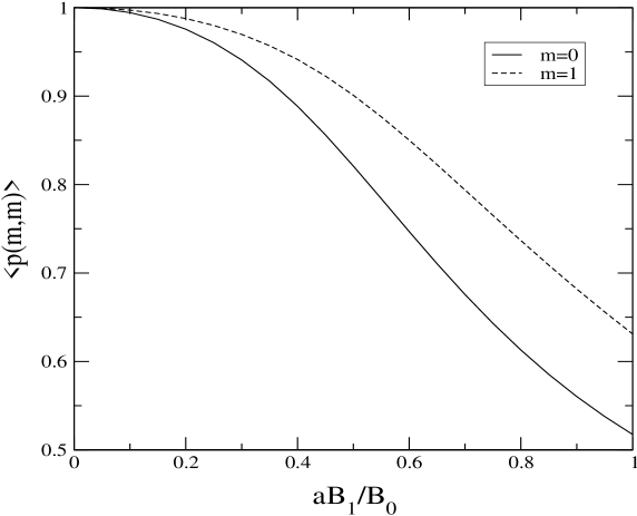
FIG. 1.: Probability that a particle with spin 1 and projection $m$ along the laboratory fixed $z$-axis is deflected according its spin projection, as a function of the parameter $aB_{1}/B_{0}$, for $m=0$ and $m=1$. The case $m=-1$ coincides with $m=1$

If we will consider the case in which $aB_{1}\ll B_{0}$, then, the angle $\beta(x,z)$ is small, and the expression above can be expressed as

$$p(m,m^{\prime}) = \delta_{m,m^{\prime}}\left(1-{I(I+1)-{m}^{2}\over 2}\beta(x,z)^{2}\right)$$ (50)

$$+ \delta_{{m}+1,m^{\prime}}\left({I(I+1)-{m}({m}+1)\over 4}\beta(x,z)^{2}\right)$$ (51)

$$+ \delta_{{m}-1,m^{\prime}}\left({I(I+1)-{m}({m}-1)\over 4}\beta(x,z)^{2}\right)$$ (52)

The Stern-Gerlach experiment is used to measure spin projections along the z-axis. Thus, if we observe a deflection corresponding to the state $m^{\prime}$, we would conclude that the spin projection along the laboratory fixed $z$-axis was $m^{\prime}$, instead of $m$. Thus, the probability that the measurement gives the incorrect result is

$$p_{e}({m})=\left({I(I+1)-{m}^{2}\over 2}\beta(x,z)^{2}\right)$$ (53)

If we average this probability over the beam probability density, we obtain

$$<p_{e}({m})>=\left({I(I+1)-{m}^{2}\over 2}\right){a^{2}B_{1}^{2}\over 2B_{0}^{2}}$$ (54)

Thus, we see that the crucial condition for the Stern-Gerlach experiment to be useful in order to measure spin projections is that the magnetic field $B_{0}$ should be much larger than the product of the gradient of this field multiplied by the size of the beam. In other words, the relative change of the magnetic field within the finite extension of the beam sould be very small. Thus, we can write

$$B_{0}\gg B_{1}a.$$ (55)

Putting together the conditions in eqs.(46,55), we have

$${B_{0}(t_{f}-t_{0})\over\hbar}\gg{B_{0}\over B_{1}a}\gg 1.$$ (56)

However, the first term is just the precession angle of the magnetic moment operator about the z-axis. This angle has to be very large, compared to 1, as a neccesary condition for eq. (56) to be valid. In this sense, our results are in agreement with the argument of Messiah [4], which points to the fact that the x-component of the magnetic moment oscillates around zero, and then it can be ignored. However, we find that this argument is not sufficient. The gradient of the magnetic field has to be such that $B_{0}\over aB_{1}$ is much smaller than the precession angle, and much larger than one.

We have performed a simulation of a beam of 1000 particles, with spin 1 and projections along the laboratory fixed $z$-axis $m=-1,0,+1$, and a probability density of having initial $(x,z)$ values given by equation (45). The particles go through an inhomogeneous magnetic field, and are deflected. The values of the magnetic field, its gradient, the length of the magnet, and the distance of the detectors are taken so that the parameter $b$, wich determines the amount of the deflection, is given as $b=4a$, in terms of the initial size of the beam. The relation of the magnetic field and its gradient is given by $B_{1}a/B_{0}=0.25$. In figure 2 we present the results of the simulation, presenting the final values of the $x$ and $z$ coordinates, in units of $a$, for different values of $m$. We find that, in general, most of the particles suffer deflections along the z axis consistent with their spin projection, but there are a few cases (corresponding to about 3% for $m=0$, and 1.5% for $m=\pm 1$), in which this is not the case. This is what we expect from figure 1. The other effect that one sees in figure 2 is a focusing effect for the particles with spin projection $m=-1$. That is related to the fact that the deflection occurs along lines that cross in the point with $(x=0,z=B_{0}/B_{1})$. The states with $m^{\prime}=-1$ tend to get close to this point, and so they focus, while the states with $m^{\prime}=1$ tend to separate from it, and so they de-focus.

FIG. 2.: Results of a simulation of 1000 particles with spin 1 and projections $m=-1,0,+1$ which go through an inhomogeneous magnetic field described by $b=4a$ and $B_{1}a/B_{0}=0.25$. The final position of the particles in the $(x,z)$ plane is represented in units of the initial beam size $a$.

In this work we have focussed in the application of Stern-Gerlach magnets as a measurement apparatus to determine the spin projection of individual atoms, assuming that the spin and the magnetic moment is previously known. We find that these experiments are not completely reliable, because the deflection is not uniquely determined by the spin projection. However, Stern-Gerlach experiments may also be used to measure the magnetic moment. In this case, one should measure the separation of the piles of particles coming from an initially unpolarized beam. Our calculations could be useful for this purpose, because they not only give the separation, but also give the shape of the different piles.

V Summary and conclusions

We describe the motion of a particle with spin in an inhomogeneous magnetic field, in a semiclassical approach. We make use of the fact that the classical trajectories are only a meaningful approach to the quantum mechanical scattering wavefunction for certain states of the internal variables, that are called Coherent Internal States. The Coherent Internal States are obtained initially as the eigenstates of the cross section matrix. Each one of these states has a trajectory that describes the time dependence of the coordinate, and an evolution operator that describes the time dependence of the internal state. The trajectory and the evolution operator are related self-consistently, because the classical force that defines the trajectory is related to expectation value of the coupling potential on the internal state, while the evolution operator is related to the coupling potential evaluated along the trajectory.

We have considered the case of a particle with a given magnetic moment, moving initially in the y-direction within a magnetic field that depends linearly on the coordinates x and z. The Coherent Internal States correspond initially to definite projections of the spin along the direction of the magnetic field evaluated at the initial point of the trajectory. The trajectory corresponding to a given spin proyection will be deflected due to the gradient in the magnetic field. The magnitude of the magnetic field observed by each particle may change as a result of the deflection of the trajectory. However, the direction of the magnetic field remains constant. Thus, the Coherent Internal State does not change as the particle moves along its trajectory.

We have considered an ensambe of particles, all moving in the y-direction, with initial x and z coordinates following a gaussian probability distribution. This illustrates a realistic situation for a beam of particles of finite size entering a Stern-Gerlach magnet. We have evaluated the trajectories followed by these particles, considering explicitly that the Coherent Internal States are different for different particles of the ensamble, because they depend on the initial values of x and z. We find that not all the particles having a given spin projection along the z-axis suffer the same deflection. This indicates that even an idealized Stern-Gerlach experiment has a finite probability of giving the wrong result as a measurement apparatus of the spin projection. The probability of error depends on the relative dispersion of the values of magnetic field within the beam size.

Acknowledgements: This work has been partially supported by the spanish CICyT, project PB98-1111

REFERENCES

- [1] R. Eisberg and R. Resnick, Quantum Physics, Wiley, 1974.
- [2] J.M. Levy-Leblond and F. Balibar, Quantics, North Holland, 1990.
- [3] E. Merzbacher, Quantum Mechanics, Wiley, 1998.
- [4] A. Messiah, Mechanique Quantique, Dunod, 1965.
- [5] S. Cruz-Barrios and J. Gómez-Camacho, Nucl. Phys. A636 (1998) 70-84
- [6] D.M. Brink, Semi-Classical Methods for Nucleus-Nucleus Scttering, Cambridge University Press, 1985.
- [7] P. Pechukas, Phys. Rev. 181 (1969) 174.
- [8] F.D. Dos Aidos, C.V. Sukumar and D.M. Brink, Nucl. Phys. A448 (1986) 333-364.
- [9] C.V. Sukumar and D.M. Brink, Nucl. Phys. A560 (1993) 863-878.
- [10] C.V. Sukumar and D.M. Brink, Nucl. Phys. A587 (1995) 413-420.
- [11] K. Alder and A. Winther, Electromagnetic Excitation, North Holland, Amsterdam, 1975.
- [12] G. R. Satchler, “Direct Nuclear Reactions”, Oxford University Press 1983, p.343.