Scharnhorst effect at oblique incidence

Abstract

We consider the Scharnhorst effect (anomalous photon propagation in the Casimir vacuum) at oblique incidence, calculating both photon speed and polarization states as functions of angle. The analysis is performed in the framework of nonlinear electrodynamics and we show that many features of the situation can be extracted solely on the basis of symmetry considerations. Although birefringence is common in nonlinear electrodynamics it is not universal; in particular we verify that the Casimir vacuum is not birefringent at any incidence angle. On the other hand, group velocity is typically not equal to phase velocity, though the distinction vanishes for special directions or if one is only working to second order in the fine structure constant. We obtain an “effective metric” that is subtly different from previous results. The disagreement is due to the way that “polarization sums” are implemented in the extant literature, and we demonstrate that a fully consistent polarization sum must be implemented via a bootstrap procedure using the effective metric one is attempting to define. Furthermore, in the case of birefringence, we show that the polarization sum technique is intrinsically an approximation.

I Introduction

In 1990 Scharnhorst demonstrated that the propagation of light in the Casimir vacuum Casimir ; Mostepanenko ; Casimir-report is characterized by an anomalous speed Sch90 . In fact photons propagating perpendicular to the plates travel at a speed $c_{\bot}$ which slightly exceeds the usual speed of light $c$ in the Minkowski vacuum Sch90 ; Bar90 ; SchBar93 ; Sch98 . The propagation of photons parallel to the plates instead occurs at the usual speed $c_{\parallel}=c$.

Unfortunately this anomalous propagation is far too small to be experimentally detectable; the relative modifications to the speed of light are of order $10^{-2}\alpha^{2}/(m_{\mathrm{e}}\,a)^{4}$, where $\alpha$ is the fine structure constant, $a$ is the distance between the plates, and $m_{\mathrm{e}}$ is the electron mass. [We work in units such that $\hbar=c=1$. Greek and Latin indices run from 0 to 3 and from 1 to 3, respectively. $\eta_{\mu\nu}=\mbox{diag}\left(-1,+1,+1,+1\right)$ denotes the Minkowski metric.] It is nevertheless an important point of principle that a quantum vacuum which is polarized by an external constraint can behave as a dispersive medium with refractive index $n(\omega)$ which remains less than unity to arbitrarily high frequency. Similar effects have been discovered in the case of quantum vacuum polarization in gravitational fields DH80 ; DS94 ; DS96 ; Shore96 , and several other situations Latorre .

It is to be emphasized that the Scharnhorst effect, albeit small, is of fundamental theoretical importance. Though the present calculations are carried out in the “soft photon” approximation (wavelengths much larger than an electron Compton wavelength) there is an argument based on dispersion relations which strongly suggests the actual signal speed is also modified (indeed, increased) SchBar93 ; Sch98 — the physics here is very different from that of the resonance-induced “apparent” superluminal velocities currently of experimental interest apparent-superluminal ; no-thing ; here we are dealing with quantum polarization induced “true” superluminal velocities, albeit well outside the realm of present day experimental technique.

A common feature of the gravitational analogs of the Scharnhorst effect is the presence of birefringence: Photons with different polarizations propagate at different speeds. Similarly in generic situations nonlinear electrodynamics often leads to birefringence Adler ; Novello ; Novello-bis . Nevertheless the occurrence of birefringence in nonlinear electrodynamics is not universal. Indeed, in the Casimir vacuum between parallel conducting plates the possibility of birefringence is tightly constrained: There is a residual (2+1) Lorentz invariance which prevents birefringence for photons that propagate parallel to the plates, and similarly there is an $O(2)$ rotational invariance that prevents birefringence for photons that propagate perpendicular to the plates. It is only for photons that propagate obliquely to the plates that there is even any possibility of birefringence. We shall be interested in a complete analysis of both propagation speed and polarization states as a function of angle, and as a side effect report the (melancholy) conclusion that birefringence is completely absent in the Casimir vacuum. As a consequence, an effective metric description is sufficient for completely specifying photon propagation in the Casimir vacuum—though it will in general not be sufficient for other more general vacuum states. The effective metric we find is subtly at variance with previous results obtained by performing a “polarization sum” Dittrich-Gies ; DGbook . The disagreement is due to the way that “polarization sums” are implemented in the extant literature, where they are defined in terms of the flat Minkowski metric. We show that in the absence of birefringence a fully consistent polarization sum must be implemented in terms of a bootstrap procedure; using as input the effective metric one is attempting to define. Furthermore, in the presence of birefringence, we demonstrate that the polarization sum technique is intrinsically an approximation. Fortunately the differences first show up at order $\alpha^{4}$, and in almost all circumstances are completely negligible.

Throughout, we emphasize the use of symmetry arguments as a way of extracting general information that is (as much as possible) independent of the particular choice of Lagrangian. Finally, we have a few words to say concerning the utility of effective metric approaches in other contexts well beyond the Casimir vacuum.

II General Formalism

Anomalous photon propagation can most easily be interpreted in terms of nonlinear electrodynamics. After integrating out virtual electron loops, the Maxwell Lagrangian should be replaced (in the absence of boundaries, at the one-loop level, and provided the distance scales defined by the field gradients and photon wavelength are much larger than the electron Compton wavelength) by Schwinger’s effective Lagrangian Schwinger

$${\cal L}_{\mathrm{Schwinger}}={\cal L}\left({\cal F},{\cal G}\right).$$ (1)

Here we have adopted the now common variables Dittrich-Gies ; DGbook

$${\cal F} \equiv \frac{1}{4}F_{\mu\nu}\;F^{\mu\nu}=\frac{1}{2}\left(\vec{B}^{2}-\vec{E}^{2}\right),$$ (2)

$${\cal G} \equiv \frac{1}{4}F_{\mu\nu}\;{}^{\star}\/F^{\mu\nu}=-\vec{E}\cdot\vec{B}.$$ (3)

The precise functional form of Schwinger’s Lagrangian will not be needed: At the end of the calculation we shall see that it is sufficient to retain only the quartic terms beyond the Maxwell Lagrangian (the Euler–Heisenberg Lagrangian Euler-Heisenberg ).

Now in the Casimir geometry between parallel plates there is one additional invariant one could consider, namely

$${\cal H} \equiv n^{\mu}F_{\mu\sigma}\;F^{\sigma\nu}\;n_{\nu}=(\vec{E}\cdot\vec{n})^{2}-(\vec{n}\times\vec{B})^{2},$$ (4)

where $n^{\mu}\equiv(0,0,0,1)$ is a unit vector orthogonal to the plates. (A similar invariant obtained by interchanging $\vec{E}$ and $\vec{B}$ is actually a redundant linear combination of the invariants $\cal F$ and $\cal H$.) In addition the coefficients in the effective Lagrangian can now explicitly depend on the $z$ coordinate. When it comes to practical calculations all these effects are suppressed by additional factors of $\hbar/(m_{\mathrm{e}}ca)$, but in the interests of generality we retain them for the time being and simply write:

$${\cal L}_{\mathrm{effective}}={\cal L}\left(F_{\mu\nu}(x),x\right).$$ (5)

That is, the considerations of the following section are not limited to the Casimir parallel plate geometry but apply whenever the soft photon approximation (and the ancillary linearization procedure and restricted eikonal approximation) make sense.

II.1 Equations of motion

The complete equations of motion for nonlinear electrodynamics consist of the Bianchi identity,

$$F_{[\mu\nu,\lambda]}=0,$$ (6)

plus the dynamical equation

$$\partial_{\nu}\left({\partial{\cal L}\over\partial F_{\mu\nu}}\right)=0.$$ (7)

We now adopt a linearization procedure: Split the electromagnetic field into a background plus a propagating photon

$$F_{\mu\nu}=F_{\mu\nu}^{\,{\mathrm{background}}}+f_{\mu\nu}^{\,{\mathrm{photon}}}.$$ (8)

Then assuming the background satisfies the equations of motion, and retaining only linear terms in the propagating photon, we have

$$f^{\,{\mathrm{photon}}}_{[\mu\nu,\lambda]}=0,$$ (9)

and

$$\partial_{\nu}\left(\left.{\partial^{2}{\cal L}\over\partial F_{\mu\nu}\;\partial F_{\alpha\beta}}\right|_{\mathrm{background}}\;f^{\,{\mathrm{photon}}}_{\alpha\beta}\right)=0.$$ (10)

On defining

$$\Omega^{\mu\nu\alpha\beta}=\left.{\partial^{2}{\cal L}\over\partial F_{\mu\nu}\;\partial F_{\alpha\beta}}\right|_{\mathrm{background}},$$ (11)

equation (10) can be rewritten in the somewhat more compact form

$$\partial_{\alpha}\left(\Omega^{\mu\alpha\nu\beta}\;f^{\,{\mathrm{photon}}}_{\nu\beta}\right)=0.$$ (12)

Note that the tensor $\Omega^{\mu\nu\alpha\beta}$ is symmetric with respect to exchange of the pairs of indices $\mu\nu$ and $\alpha\beta$, and antisymmetric with respect to exchange of indices within each pair.

We now apply a restricted form of the eikonal approximation by introducing a slowly varying amplitude $f_{\mu\nu}$ and a rapidly varying phase $\phi$:

$$f^{\,{\mathrm{photon}}}_{\mu\nu}=f_{\mu\nu}\;{\rm e}^{{\mathrm{i}}\phi}.$$ (13)

The wave vector (actually a one-form, but we shall loosely refer to both vectors and one-forms as “vectors” in the text, because of the mapping provided by $\eta_{\mu\nu}$ and its inverse $\eta^{\mu\nu}$) is then defined as $k_{\mu}=\partial_{\mu}\phi$. This approximation is similar to, but not quite identical with, the usual eikonal approximation. This is because one assumes that $\phi$ varies on scales much smaller than those of the background, while, on the other hand, use of the Lagrangian (5) also implies that the components of $k$ are much smaller than the values fixed by the electron mass (soft-photon regime). Under these hypotheses,

$$\Omega^{\mu\alpha\nu\beta}\;k_{\alpha}\;f_{\nu\beta}=0.$$ (14)

But the background field is itself subject to quantum fluctuations, and to take this into account the coefficients of this equation are identified with the expectation value of the corresponding quantum operators in the background state $|\psi\rangle$:

$$\langle\psi|\Omega^{\mu\alpha\nu\beta}|\psi\rangle\;k_{\alpha}\;f_{\nu\beta}=0.$$ (15)

In taking this expectation value we are using the fact that the fluctuations in the background fields are determined by the geometry (in the specific case of the Casimir geometry, by the distance between the plates), so that in the spirit of the restricted eikonal approximation there is a separation of scales between the background fluctuations and the propagating photon.

The Bianchi identity (9) constrains $f_{\mu\nu}$ to be of the form

$$f_{\mu\nu}=k_{\mu}\;a_{\nu}-k_{\nu}\;a_{\mu}\,,$$ (16)

where we have introduced the gauge potential $a$ for the propagating field. Inserting (16) into (15) we find

$$\langle\psi|\Omega^{\mu\alpha\nu\beta}|\psi\rangle\;k_{\alpha}\;k_{\beta}\;a_{\nu}=0.$$ (17)

In general, the tensorial quantity $\langle\psi|\Omega^{\mu\alpha\nu\beta}|\psi\rangle$ can be decomposed into an isotropic part plus anisotropic contributions, that we group together into a term $\Delta^{\mu\alpha\nu\beta}$ with the same symmetries as $\Omega^{\mu\alpha\nu\beta}$:

$$\langle\psi|\Omega^{\mu\alpha\nu\beta}|\psi\rangle=d_{1}\,\big{(}\eta^{\mu\nu}\;\eta^{\alpha\beta}-\eta^{\mu\beta}\;\eta^{\alpha\nu}\big{)}+\Delta^{\mu\alpha\nu\beta},$$ (18)

where $d_{1}$ is a function that can in principle be computed directly from the effective Lagrangian.

II.2 Dispersion relations

Equation (17) represents a condition for $a$ as a function of $k$ — it constrains $a$ to be an eigenvector, with zero eigenvalue, of the $k$-dependent matrix

$$A^{\mu\nu}(k)=\langle\psi|\Omega^{\mu\alpha\nu\beta}|\psi\rangle\;k_{\alpha}\;k_{\beta}.$$ (19)

Any non-zero solution corresponds to a physically possible field polarization, that can be identified by a unit polarization vector $\epsilon$ (provided $a$ is not a null vector — a possibility that can always be avoided by a suitable gauge choice).

A necessary and sufficient condition for the eigenvalue problem $A^{\mu\nu}\,a_{\nu}=0$ to have non-zero solutions is $\mbox{det}\left(A^{\mu\nu}\right)=0$; however, this gives us no information at all. Indeed, any $a$ parallel to $k$ is always a non-zero solution, so the condition $\mbox{det}\left(A^{\mu\nu}\right)=0$ is actually an identity. On the other hand, $a\parallel k$ is merely an unphysical gauge mode that corresponds to $f_{\mu\nu}=0$ by (16), so we need to find other, physically meaningful, solutions of the eigenvalue problem. To this end, we exploit gauge invariance under $a\to a+\lambda\,k$ and fix a gauge, thus removing the spurious modes. It is particularly convenient to adopt the temporal gauge $a_{0}=0$. Then we can define a polarization vector $\epsilon_{\mu}\equiv a_{\mu}/\left(a_{\nu}a^{\nu}\right)^{1/2}$, and the eigenvalue problem $A^{\mu\nu}\,\epsilon_{\nu}=0$ splits into the equation

$$A^{0i}\,\epsilon_{i}=0,$$ (20)

plus the reduced eigenvalue problem

$$A^{ij}\,\epsilon_{j}=0\,.$$ (21)

The latter admits a nontrivial solution only if

$$\mbox{det}\left(A^{ij}\right)=0.$$ (22)

The condition (22) plays the same role as the Fresnel equation in crystal optics landau — it is a scalar equation for $k$ and thus gives the dispersion relation for light propagating in our “medium”.

An explicit calculation (see Appendix B) gives

$$\mbox{det}\left(A^{ij}\right)=\omega^{2}\;{\cal P}_{4}(k),$$ (23)

where $\omega\equiv-k_{0}$ and ${\cal P}_{4}(k)$ is a homogeneous fourth-order polynomial in the variables $\omega$ and $k_{i}$. This means that in the most general case there are four dispersion relations, corresponding to the four roots of the equation

$${\cal P}_{4}(k)=0.$$ (24)

But, if $k=(-\omega,\vec{k})$ is a root then so is $-k=(\omega,-\vec{k})$; thus, by CPT invariance, only two of these dispersion relations are physically distinct.

Different polarization states are represented by linearly independent solutions of the eigenvalue problem (21), under the condition (22). [Obviously, (20) cannot be independent of (21), since we know that $\mbox{det}\left(A^{\mu\nu}\right)\equiv 0$.] Thus, the space of polarizations is at most two-dimensional. Since (22) gives rise to two dispersion relations, the polarization states actually satisfy two (in general, different) eigenvalue equations,

$$\overline{A}_{(r)}^{\,\mu\nu}\;\epsilon^{\,(r)}_{\;\nu}=0\,,$$ (25)

where $r=1,2$ labels the dispersion relations and $\overline{A}_{(r)}^{\,\mu\nu}$ is obtained from $A^{\mu\nu}$ by imposing the corresponding condition on $k$. Thus, in the general case, modes of the field with different polarizations have different dispersion relations, hence propagate in different ways; this leads to the phenomenon of birefringence Adler ; Novello ; Novello-bis .

In some special cases (in particular, this behaviour is quite common in nonlinear electrodynamics) the polynomial ${\cal P}_{4}(k)$ factorizes into two quadratic forms,

$${\cal P}_{4}(k)=\bigl{(}\gamma_{(1)}^{\,\mu\nu}\;k_{\mu}\,k_{\nu}\bigr{)}\;\bigl{(}\gamma_{(2)}^{\,\alpha\beta}\;k_{\alpha}\,k_{\beta}\bigr{)},$$ (26)

in which case we obtain two second-order dispersion relations:

$$\gamma_{(1)}^{\,\mu\nu}k_{\mu}k_{\nu}=0\quad\mbox{and}\quad\gamma_{(2)}^{\,\mu\nu}k_{\mu}k_{\nu}=0.$$ (27)

II.3 Effective metric

We now want to consider the special situation in which not only does (26) hold, but also $\gamma_{(1)}^{\,\mu\nu}=\gamma_{(2)}^{\,\mu\nu}$. (That is, the fourth-order polynomial ${\cal P}_{4}(k)$ is a perfect square.) In this case one ends up with a single quadratic dispersion relation of the familiar form

$$\gamma^{\,\mu\nu}\,k_{\mu}\,k_{\nu}=0,$$ (28)

where $\gamma^{\,\mu\nu}$ is some symmetric tensor. It should be clear from our previous discussion that a necessary condition for this to happen is the absence of birefringence. Remarkably, we see that the wave vector is now null with respect to a (unique) “effective inverse metric” $\gamma^{\,\mu\nu}$. Therefore, the propagation of light can be described in terms of an effective geometry, defined by the metric tensor ${\rm g}_{\mu\nu}$ obtained by inverting $\gamma^{\,\mu\nu}$, such that $\gamma^{\,\mu\nu}{\rm g}_{\nu\rho}=\delta^{\,\mu}{}_{\rho}$.

(Warning: Even when an effective metric is defined, we always raise and lower indices using the flat Minkowski metric $\eta_{\mu\nu}$. In particular, note that ${\rm g}_{\mu\nu}\neq\eta_{\mu\rho}\,\eta_{\nu\sigma}\gamma^{\,\rho\sigma}$; this justifies our use of different symbols, $\rm g$ and $\gamma$, for the effective metric and its inverse.)

This situation implies that $\langle\psi|\Omega^{\mu\alpha\nu\beta}|\psi\rangle$ must be algebraically constructible solely in terms of $\gamma^{\,\mu\nu}$. In view of the symmetries of $\Omega^{\mu\alpha\nu\beta}$ we know, without need for detailed calculation, that it must be of the form

$$\langle\psi|\Omega^{\mu\alpha\nu\beta}|\psi\rangle=\Lambda\bigl{(}\gamma^{\,\mu\nu}\;\gamma^{\,\alpha\beta}-\gamma^{\,\mu\beta}\;\gamma^{\,\nu\alpha}\bigr{)}$$ (29)

for some function $\Lambda$.

Conversely, if $\Omega^{\mu\alpha\nu\beta}$ is of the form (29), then the matrix (19) is

$$A^{\mu\nu}=\Lambda\,\left[\gamma^{\,\mu\nu}\bigl{(}\gamma^{\,\alpha\beta}\,k_{\alpha}\,k_{\beta}\bigr{)}-\bigl{(}\gamma^{\,\mu\alpha}\,k_{\alpha}\bigr{)}\bigl{(}\gamma^{\,\nu\beta}\,k_{\beta}\bigr{)}\right],$$ (30)

and the photon propagation equation $A^{\mu\nu}\,a_{\nu}=0$ becomes

$$\bigl{(}\gamma^{\,\alpha\beta}\,k_{\alpha}\,k_{\beta}\bigr{)}\gamma^{\,\mu\nu}\,a_{\nu}-\bigl{(}\gamma^{\,\alpha\beta}\,a_{\alpha}\,k_{\beta}\bigr{)}\gamma^{\,\mu\nu}\,k_{\nu}=0.$$ (31)

This equation is obviously satisfied by the uninteresting gauge modes $a\parallel k$, with no constraints on $k$. Solutions corresponding to a non-vanishing $f_{\mu\nu}$ exist only if the coefficient of $\gamma^{\,\mu\nu}\,a_{\nu}$ is zero, i.e., if (28) holds. Thus, the two polarization states propagate with the same dispersion relation (28), and there is no birefringence.

Substituting (28) back into the propagation equation (31) we find another relationship typical of this case,

$$\gamma^{\,\mu\nu}\,k_{\mu}\,a_{\nu}=0.$$ (32)

Formally, the above equation looks like a gauge condition. This might seem puzzling, because nowhere in the present subsection have we fixed a gauge. In fact, (32) is a consequence of the dynamical equation $A^{\mu\nu}\,a_{\nu}=0$, when the “on-shell” condition (28) is satisfied, and it does not imply any gauge fixing.

Finally, it is interesting to notice that there is now a self-consistency or “bootstrap” condition,

$$3\,\Lambda\,\gamma^{\,\mu\nu}=\langle\psi|\Omega^{\mu\alpha\nu\beta}|\psi\rangle\;{\rm g}_{\alpha\beta}.$$ (33)

This can be re-stated directly in terms of the fundamental coefficients as

$$3\,\Lambda\,\gamma^{\,\mu\nu} = d_{1}\;\eta^{\mu\nu}\left(\eta^{\alpha\beta}\;{\rm g}_{\alpha\beta}\right)-d_{1}\;\eta^{\mu\alpha}\;{\rm g}_{\alpha\beta}\;\eta^{\beta\nu}$$ (34)

$$\qquad+\Delta^{\mu\alpha\nu\beta}\;{\rm g}_{\alpha\beta}.$$

We stress that these relations depend only on the assumed existence of a single unique effective metric ${\rm g}_{\mu\nu}$ — they do not make any reference to other specifics of the quantum state.

III Casimir vacuum

Let us now consider a region of empty space delimited by two perfectly conducting parallel plates placed orthogonal to the $z$ axis at positions $z=z_{0}$ and $z=z_{0}+a$, in the quantum state $|\psi\rangle\to|C\rangle$ corresponding to the Casimir vacuum Casimir ; Mostepanenko ; Casimir-report .

III.1 Symmetries and effective metric

In the Casimir vacuum considerable information can be extracted by using only symmetry considerations, similarly to what Bryce DeWitt did for the stress-energy-momentum tensor in reference DeWitt . Always working in the soft photon approximation, the presence of a preferred direction and the symmetry of the configuration allow us to claim that the function $d_{1}$ can only depend on the $z$ coordinate, and to write $\Delta^{\mu\alpha}{}_{\nu\beta}$ in the form

$$\Delta^{\mu\alpha}{}_{\nu\beta} = d_{2}(z)\;\big{(}\delta^{\mu}{}_{\nu}\;n^{\alpha}\;n_{\beta}-\delta^{\mu}{}_{\beta}\;n^{\alpha}\;n_{\nu}$$ (35)

$$\quad+\delta^{\alpha}{}_{\beta}\;n^{\mu}\;n_{\nu}-\delta^{\alpha}{}_{\nu}\;n^{\mu}\;n_{\beta}\big{)},$$

where $d_{2}(z)$ is another function. The calculation of $d_{1}(z)$ and $d_{2}(z)$ in this case is straightforward, using identities that follow from (18) and (35):

$$d_{1}(z)=\frac{1}{6}\left\langle C\left|\Omega^{\mu\nu}{}_{\mu\nu}-2\,\Omega^{\mu\nu}{}_{\alpha\nu}\;n_{\mu}\;n^{\alpha}\right|C\right\rangle;$$ (36)

$$d_{2}(z)=-\frac{1}{6}\left\langle C\left|\Omega^{\mu\nu}{}_{\mu\nu}-4\,\Omega^{\mu\nu}{}_{\alpha\nu}\;n_{\mu}\;n^{\alpha}\right|C\right\rangle.$$ (37)

On defining the function

$$\xi(z)\equiv{d_{2}(z)\over d_{1}(z)},$$ (38)

and the tensor

$$\gamma^{\,\mu\nu}=\eta^{\mu\nu}+\xi(z)\,n^{\mu}n^{\nu},$$ (39)

$\langle C|\Omega^{\mu\alpha\nu\beta}|C\rangle$ takes the particularly simple form

$$\langle C|\Omega^{\mu\alpha\nu\beta}|C\rangle=d_{1}(z)\;\bigl{(}\gamma^{\,\mu\nu}\;\gamma^{\,\alpha\beta}-\gamma^{\,\mu\beta}\;\gamma^{\,\nu\alpha}\bigr{)}.$$ (40)

Thus, from the discussion in subsection II.3, we deduce without further argument that there is no birefringence, and that $\gamma^{\,\mu\nu}$ given in (39) plays the role of an effective inverse metric for the propagation of light in the Casimir vacuum. The corresponding effective metric is

$${\rm g}_{\mu\nu}=\eta_{\mu\nu}-\frac{\xi(z)}{1+\xi(z)}\,n_{\mu}n_{\nu}.$$ (41)

We stress that for this derivation of the effective metric to make sense it is necessary that the spatial variation in $\xi(z)$ be compatible with the restricted eikonal approximation: that is $\xi(z)$ should vary slowly on the scale of the photon wavelength. This is certainly true for QED at lowest nontrivial order where we shall soon see that $\xi$ is in fact independent of $z$.

The conclusion about the absence of birefringence can also be obtained more explicitly. Choosing the temporal gauge, and following the steps outlined in the general analysis of subsection II.2, equation (20) becomes

$$\gamma^{\,ij}\,k_{i}\,\epsilon_{j}=0,$$ (42)

which also follows from (32) when $\epsilon_{0}=0$. A tedious but straightforward calculation gives

$$\mbox{det}\left(A^{ij}\right)=-\left(1+\xi\right)\;d_{1}^{\,3}\;\omega^{2}\;\bigl{(}\gamma^{\,\mu\nu}\,k_{\mu}\,k_{\nu}\bigr{)}^{2}.$$ (43)

Thus the dispersion relation determined from (22) takes in this case the form (28), as expected.

We note here that, although an equation of the form (28) has been already obtained by Dittrich and Gies Dittrich-Gies , the expression for the effective metric underlying their dispersion relation is subtly at variance with our results (39) and (41). We shall comment about the reason for this discrepancy in Appendix C.

III.2 Polarization states

In order to explicitly find the polarization states, let us evaluate (19) using the expression for $\langle C|\Omega^{\mu\alpha\nu\beta}|C\rangle$ and (28), and then consider the reduced eigenvalue problem (21). We find that $\vec{\epsilon}$ must be a solution of the problem $\overline{A}^{\,ij}\,\epsilon_{j}=0$, where

$$\overline{A}^{\,ij}=-\gamma^{\,il}\,k_{l}\;\gamma^{\,jm}\,k_{m}.$$ (44)

This eigenvalue problem, however, is manifestly equivalent to the single equation (42), which is thus the only constraint that the polarization states must satisfy. Therefore, the space of polarization states is two-dimensional, as expected.

A basis for such a space can be easily constructed by considering generic propagation in the $xz$ plane [not a restrictive hypothesis, because of $O(2)$ invariance with respect to rotations around the $z$ axis], described by the 3-vector (these are taken to be covariant components, index down):

$$\vec{k}=\left(|\vec{k}|\sin\theta,0,|\vec{k}|\cos\theta\right).$$ (45)

Equation (42) then becomes

$$\sin\theta\;\epsilon_{1}+\left(1+\xi\right)\,\cos\theta\;\epsilon_{3}=0,$$ (46)

so two independent polarizations are:

$$\vec{\epsilon}^{\;(1)} = (0,1,0);$$

$$\vec{\epsilon}^{\;(2)} = \frac{1}{N(\theta)}\bigl{(}\left(1+\xi\right)\cos\theta,0,-\sin\theta\bigr{)},$$ (47)

where

$$N(\theta)\equiv\left(1+2\,\xi\,\cos^{2}\theta+\xi^{2}\cos^{2}\theta\right)^{1/2}$$ (48)

is a normalization coefficient. Note in particular that $\vec{\epsilon}^{\;(2)}$ is not perpendicular to $\vec{k}$ when viewed in terms of the Minkowski metric $\eta^{\mu\nu}$, though they are perpendicular when viewed in terms of the effective metric $\gamma^{\,\mu\nu}$. Furthermore we have chosen to make $\vec{\epsilon}^{\;(2)}$ a unit vector with respect to the Minkowski metric, not with respect to the effective metric.

III.3 Phase, signal, and group velocities

If $\vec{k}$ has the form (45), equation (28) becomes (the norms are with respect to the Euclidean spatial metric induced by $\eta_{\mu\nu}$):

$$\omega^{2}=|\vec{k}|^{2}+\xi\;|\vec{k}|^{2}\;\cos^{2}\theta.$$ (49)

The phase velocity is given by

$$v_{\mathrm{phase}}(\theta)=\frac{\omega}{|\vec{k}|}=\left(1+\xi\,\cos^{2}\theta\right)^{1/2},$$ (50)

and is independent of the polarization. This is again a consequence of the fact that the quantity $\gamma^{\,\mu\nu}\,k_{\mu}\,k_{\nu}$ appears squared in $\mbox{det}\left(A^{ij}\right)$, so equation (22) describes a degenerate fourth-degree surface in the space of the vectors $\vec{k}/\omega$. Hence, there is only one dispersion relation, equation (49), independent of the polarization state, and only one phase speed for each value of $|\vec{k}|$. This confirms that birefringence does not take place in the Casimir vacuum.

Note that if $\xi>0$ and $\theta\neq\pi/2$, we have $v_{\mathrm{phase}}(\theta)>1$. Since, in the limit $\omega\to+\infty$, $v_{\mathrm{phase}}$ equals the front velocity (signal velocity) Sch98 , one is tempted to argue that the propagation is superluminal for all values of $\theta$ different from $\pi/2$. This conclusion can also be inferred directly from (28), which for $\xi>0$ implies that $k$ is timelike (with respect to the undisturbed Minkowski metric). Since $k$ can also be interpreted as the four-vector orthogonal to a surface of discontinuity of the field Novello ; Novello-bis , it follows that such a surface is spacelike (with respect to the Minkowski metric), i.e., that electromagnetic signals travel “faster than light”. (This phrasing is standard but unfortunate, and is logically indefensible. It should always be interpreted in the sense “faster than light would have travelled in an undisturbed portion of normal vacuum”.) Equivalently, (41) implies that for $\xi>0$ the lightcones of the effective metric ${\rm g}_{\mu\nu}$ are wider than those of the Minkowski metric $\eta_{\mu\nu}$. Unfortunately, while it is certainly true that our treatment is valid at high frequencies (with respect to those associated to the background scales), it nevertheless also requires $\omega\ll m_{\mathrm{e}}$ — the condition under which one can use the Lagrangian (1) —, so we have no direct information about the strict $\omega\to+\infty$ limit. See, however, reference SchBar93 for an indirect argument based on the Kramers–Kronig dispersion relation that combined with the present calculation is sufficient to establish superluminal propagation for the signal velocity. In the special case $\theta=\pi/2$ one has $\eta^{\mu\nu}k_{\mu}k_{\nu}=0$: Photons propagating parallel to the plates travel at the standard speed of light.

The group velocity is a little tricky, it equals

$$v^{i}_{\mathrm{group}}\equiv{\partial\omega\over\partial k_{i}}=\frac{1}{\omega}\left[k^{i}+\xi\;(k\cdot n)\;n^{i}\right],$$ (51)

so equations (45) and (50) give

$$\vec{v}_{\mathrm{group}}(\theta)=\frac{1}{v_{\mathrm{phase}}(\theta)}\bigl{(}\sin\theta,0,(1+\xi)\cos\theta\bigr{)}.$$ (52)

In particular, the group velocity $\vec{v}_{\mathrm{group}}$ is not parallel to the wave-vector $\vec{k}$, though it is always orthogonal to the polarization vector. Taking the norm (in the physical Minkowski metric),

$$v_{\mathrm{group}}(\theta)={N(\theta)\over v_{\mathrm{phase}}(\theta)}=\left[{1+(2\xi+\xi^{2})\cos^{2}\theta\over 1+\xi\;\cos^{2}\theta}\right]^{1/2}.$$ (53)

The group speed is at all angles slightly greater than (or at worst equal to) the phase speed. (See figure 1.) Indeed

$$v_{\mathrm{group}}^{2}(\theta)=v_{\mathrm{phase}}^{2}(\theta)+{\xi^{2}\cos^{2}\theta\;\sin^{2}\theta\over v_{\mathrm{phase}}^{2}(\theta)}.$$ (54)

(See figure 2.) Care should be taken to realize that here $\theta$ is the angle between the wave vector and the normal, and is not quite the same as the direction of propagation of the wave packet. Fortunately at both normal incidence ($\theta=0$) and parallel propagation ($\theta=\pi/2$) the distinction between group and phase velocities disappears. Furthermore, as we shall see below, if we work to second order in the fine structure constant, the difference between group and phase speed is negligible at all angles, although a difference of order $\alpha^{2}$ still remains between the directions of $\vec{v}_{\mathrm{group}}$ and $\vec{k}$. The group velocity (53) is greater than 1 when $\xi>0$. Thus, the group speed is larger than 1 whenever the phase speed is, although in general their individual values are different.

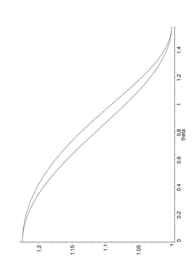
Figure 1: Group and phase speeds as a function of angle, from $\theta=0$ to $\theta=\pi/2$ radians. (The group speed is the upper curve.) For clarity we have greatly exaggerated the physically expected value of $\xi$ by setting $\xi=1/2$.

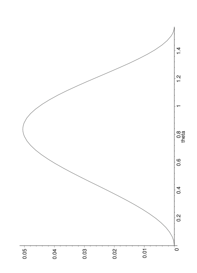
Figure 2: Difference between the squares of the group and phase speeds as a function of angle, from $\theta=0$ to $\theta=\pi/2$ radians. For clarity we have greatly exaggerated the physically expected value of $\xi$ by setting $\xi=1/2$.

IV Size of the effect

So far we have seen that, based solely on symmetry considerations, we can eliminate the possibility of birefringence in the Casimir vacuum and place strong constraints on the general features of photon propagation in this vacuum. Our results are in fact generic to any form of nonlinear electrodynamics subject to the boundary conditions appropriate for the Casimir vacuum, and are not specifically restricted to QED. Where QED is important is in determining the specific form of the functions $d_{1}(z)$ and $d_{2}(z)$, which determine $\xi(z)$, and hence determine the size (but not the qualitative features) of the Scharnhorst effect.

Unless one wants to perform calculations to orders higher than $\alpha^{2}$, it is sufficient to consider the Euler–Heisenberg Lagrangian Euler-Heisenberg which, in the ${\cal F}$–${\cal G}$ formalism adopted above, takes the form

$${\cal L}_{\rm EH}=-\frac{1}{4\pi}\;{\cal F}+c_{1}\;{\cal F}^{2}+c_{2}\;{\cal G}^{2},$$ (55)

with

$$c_{1}=\frac{\alpha^{2}}{90\pi^{2}m^{4}_{\mathrm{e}}},\qquad c_{2}=\frac{7\alpha^{2}}{360\pi^{2}m^{4}_{\mathrm{e}}}.$$ (56)

The terms proportional to ${\cal F}^{2}$ and ${\cal G}^{2}$ of this Lagrangian are quartic in the field, and describe the low-energy limit of the box diagram in QED, when four photons couple to a single virtual electron loop. Thus, the Lagrangian (55) is only accurate to order $\alpha^{2}$, and it is meaningless to retain higher order terms within this model.

In particular, deviations from (3+1) Lorentz symmetry due to the presence of the plates (the plates reduce the symmetry group to that of (2+1) Lorentz invariance) must on physical grounds vanish as the plate separation goes to infinity, where one must recover the full (3+1) Lorentz symmetry. On dimensional grounds this implies that such terms will be suppressed by some function of $\hbar/(m_{e}ca)$ and can, to lowest nontrivial order, be neglected in the effective Lagrangian. On the other hand, even for lowest nontrivial order in the effective Lagrangian (that is, for the Euler–Heisenberg Lagrangian), the presence of the plates leads to a nontrivial expectation value for $\langle C|F_{\mu\nu}\;F_{\alpha\beta}|C\rangle$ and will in this way contribute to the effective metric.

For the Euler–Heisenberg Lagrangian, the tensor $\Omega^{\mu\nu}{}_{\alpha\beta}$ is

$$\Omega^{\mu\nu}{}_{\alpha\beta} = \left(-{1\over 16\pi}+{c_{1}\;{\cal F}\over 2}\right)\;\big{(}\delta^{\mu}{}_{\alpha}\;\delta^{\nu}{}_{\beta}-\delta^{\mu}{}_{\beta}\;\delta^{\nu}{}_{\alpha}\big{)}$$ (57)

$$+{c_{2}\;{\cal G}\over 2}\;\epsilon^{\mu\nu}{}_{\alpha\beta}$$

$$+{c_{1}\over 2}\;F^{\mu\nu}\;F_{\alpha\beta}+{c_{2}\over 2}\;{}^{\star}\/F^{\mu\nu}\;{}^{\star}\/F_{\alpha\beta},$$

so in the Casimir vacuum

$$d_{1}(z)=-\frac{1}{16\pi}+O(\alpha^{2})$$ (58)

while $d_{2}(z)$ is of order $\alpha^{2}$. Hence, to first order in $\alpha^{2}$, we have $\xi(z)=-16\pi\,d_{2}(z)$, and

$$v_{\mathrm{phase}}(\theta)=v_{\mathrm{group}}(\theta)=1-8\pi d_{2}(z)\;\cos^{2}\theta.$$ (59)

Though in principle the coefficient $d_{2}(z)$ could depend on $z$, the position relative to the two plates, we shall see that in the specific case of the Casimir vacuum it is simply a position-independent number.

To establish this, start with (37), and insert the specific form (57). Using the algebraic identity Schwinger ; Dittrich-Gies

$${}^{\star}\/F^{\mu\nu}\;{}^{\star}\/F_{\alpha\nu}=F^{\mu\nu}\;F_{\alpha\nu}-2\,{\cal F}\,\delta^{\mu}{}_{\alpha},$$ (60)

one easily gets

$$\Omega^{\mu\nu}{}_{\alpha\nu} = \left(-{1\over 16\pi}+{c_{1}\;{\cal F}\over 2}\right)\;3\;\delta^{\mu}{}_{\alpha}$$ (61)

$$+2\pi\left(c_{1}+c_{2}\right)T^{\mu}{}_{\alpha}+{\left(c_{1}-c_{2}\right){\cal F}\over 2}\,\delta^{\mu}{}_{\alpha},$$

where $T^{\mu}{}_{\alpha}$ is Maxwell’s stress-energy-momentum tensor. Performing the indicated traces, and using the fact that the Maxwell stress-energy tensor is traceless, we find

$$d_{2}(z)=\frac{4\pi}{3}(c_{1}+c_{2})\;\left\langle C\left|T_{zz}\right|C\right\rangle.$$ (62)

The symmetries of the Casimir vacuum stress-energy (as analyzed for instance by DeWitt DeWitt ), then imply

$$d_{2}(z)=4\pi(c_{1}+c_{2})\;\left\langle C\left|T_{00}\right|C\right\rangle.$$ (63)

Finally the well-known result $\langle C|T_{00}|C\rangle=-\pi^{2}/720a^{4}$ allows us to write

$$d_{2}=-\frac{11\pi\alpha^{2}}{64800\,a^{4}\,m^{4}_{\mathrm{e}}}.$$ (64)

And in particular, this implies $d_{2}(z)$ is position independent. Thus, at first order in $\alpha^{2}$,

$$v_{\mathrm{phase}}(\theta)=v_{\mathrm{group}}(\theta)=1+\frac{11\pi^{2}\alpha^{2}}{8100\,a^{4}\,m^{4}_{\mathrm{e}}}\,\cos^{2}\theta.$$ (65)

This expression reproduces Scharnhorst’s result in the case $\theta=0$, generalizing it to an arbitrary direction of propagation. It is interesting to notice that the correction is essentially determined by the expectation value of the energy density, $\langle C|T_{00}|C\rangle$, in agreement with the general results of Latorre ; Dittrich-Gies .

V Conclusions

We have outlined a general scheme that allows one to write down the dispersion relation, and to find the polarization states, for electromagnetic radiation propagating in a region where nonlinear effects cannot be ignored. The deviations from the behaviour in Maxwell’s theory are completely described by the tensorial quantity $\Delta^{\mu\alpha\nu\beta}$, that has its origin in the anisotropy of the medium. In particular, we have investigated the case of propagation in the Casimir vacuum, where there is a privileged direction in space, identified by a unit vector $n$. We have seen that symmetry considerations alone imply that $\Delta^{\mu\alpha}{}_{\nu\beta}$ must be of the form (35). This, in turn, implies that there is only one value for the speed of light, independent of the polarization. Thus, the possibility of birefringence in the Casimir vacuum is completely ruled out by very general arguments (the abstract form of the Lagrangian for nonlinear electrodynamics, plus the tensor structure of $\Delta^{\mu\alpha}{}_{\nu\beta}$ dictated by the geometry). Because of its generality, this conclusion applies not just to QED itself but to arbitrary types of nonlinear electrodynamics (such as for instance, Born–Infeld theories).

How are we to interpret this result in view of the fact that nonlinear electrodynamics generically does lead to birefringence Adler ; Novello ; Novello-bis ? The key point is that in those analyses the background field $(F^{\mu\nu})_{\mathrm{background}}$ is nonzero. More generally, even after averaging over quantum fluctuations of the background, $\langle\psi|F^{\mu\nu}|\psi\rangle\neq 0$ in the quantum state appropriate to those analyses. In the Casimir vacuum on the other hand, the expectation values linear in the field do vanish, $\langle C|F^{\mu\nu}|C\rangle=0$, and it is only the quadratic expectation values (and higher) that are nonzero ($\langle C|\Omega^{\mu\nu\alpha\beta}|C\rangle\neq 0$). This key difference makes the analyses of Adler ; Novello ; Novello-bis inapplicable to the Casimir vacuum—technically speaking, the polarization basis used in those papers fails to be meaningful for the Casimir vacuum. On the other hand, the discussion of the present paper could be easily adapted to treat light propagation in the presence of an electromagnetic background field. It is sufficient to keep in mind that in this case there is a preferred 2-dimensional plane defined by the 2-form $\langle\psi|F^{\mu\nu}|\psi\rangle$. Correspondingly, the form of $\Delta^{\mu\alpha\nu\beta}$ will be more complicated [see (67)].

We reiterate that the absence of birefringence is crucial for the use of the “effective geometry” approach (adopted in this type of context by Latorre et al Latorre , and further developed by Novello et al Novello , and by Dittrich and Gies Dittrich-Gies ). Only if the propagation of light does not depend on its polarization and is thus, in a sense, universal, it is meaningful to describe it by a single effective metric. As a consequence of our analysis, photon propagation in the Casimir vacuum can indeed be phrased entirely in terms of the effective metric (39). This observation is potentially important in that “effective metric” approaches similar in spirit to the above are currently attracting attention in fields as diverse as acoustics Unruh ; Acoustics , optics Leonhardt ; Optics , superfluid quasiparticles Volovik , and Bose–Einstein condensates Garay .

Finally, we mention related work on the light cone condition for a thermalized QED vacuum due to Gies Gies (wherein the analysis implicitly relies on taking the quantum expectation value of $\Omega^{\mu\nu\alpha\beta}$ in a manner somewhat analogous to the present paper), and intriguing results on photon propagation in rather general linear theories in classical backgrounds due to Obukhov and co-workers Obukhov-Hehl ; Hehl ; Obukhov .

Appendix A Connection with other formulations

We have tried to set up the formalism in a streamlined and self-contained manner. Nevertheless to aid comparison with other results in the literature it is useful to give the explicit form of the tensor $\Omega^{\mu\nu\alpha\beta}$ for generic Schwinger-like Lagrangians of the form (1). For such Lagrangians

$$\Omega^{\mu\nu\alpha\beta} = {1\over 4}\;\left(\partial_{\cal F}{\cal L}\right)\;\big{(}\eta^{\mu\alpha}\;\eta^{\nu_{\beta}}-\eta^{\mu\beta}\;\eta^{\nu\alpha}\big{)}$$ (66)

$$+{1\over 4}\;\left(\partial_{\cal G}{\cal L}\right)\;\epsilon^{\mu\nu\alpha\beta}+{1\over 4}\;M^{\mu\nu\alpha\beta},$$

where

$$M^{\mu\nu\alpha\beta} = F^{\mu\nu}\;F^{\alpha\beta}\;\left(\partial^{2}_{\cal F}{\cal L}\right)+{}^{\star}\/F^{\mu\nu}\;{}^{\star}\/F^{\alpha\beta}\;\left(\partial^{2}_{\cal G}{\cal L}\right)$$ (67)

$$+\left(F^{\mu\nu}\;{}^{\star}\/F^{\alpha\beta}+{}^{\star}\/F^{\mu\nu}\;F^{\alpha\beta}\right)\partial_{\cal FG}{\cal L}$$

has the same symmetries as $\Omega^{\mu\nu\alpha\beta}$.

As soon as one inserts this tensor into the photon equation of motion (14), the completely antisymmetric part proportional to the Levi–Civita tensor drops out, because of the Bianchi identity (9). The remaining pieces reproduce the photon equation of motion in the perhaps more usual form considered by Dittrich and Gies Dittrich-Gies , or Novello and co-workers Novello ; Novello-bis .

Also note that, depending on the details of the geometry and the quantum state, $M^{\mu\nu\alpha\beta}$ can contribute to both $d_{1}$ and to $\Delta^{\mu\nu\alpha\beta}$.

Appendix B Fresnel equation in nonlinear electrodynamics

Our purpose is to prove equation (23). The spatial components of the matrix (19) are

$$A^{ij} = \omega^{2}\;\langle\psi|\Omega^{i0j0}|\psi\rangle-\omega\;k_{m}\;\langle\psi|\Omega^{i0jm}+\Omega^{imj0}|\psi\rangle$$ (68)

$$\qquad+k_{m}k_{n}\;\langle\psi|\Omega^{imjn}|\psi\rangle.$$

Let us define the unit vector $\hat{k}=\vec{k}/|\vec{k}|$. Then the components of $A^{ij}$ in a basis with one axis directed along $\hat{k}$ are

$$A^{ij}\hat{k}_{j}=\omega^{2}\;\langle\psi|\Omega^{i0j0}|\psi\rangle\;\hat{k}_{j}-\omega\;k_{m}\;\langle\psi|\Omega^{imj0}|\psi\rangle\;\hat{k}_{j}\equiv\omega\;V^{i}.$$ (69)

In particular

$$A^{ij}\hat{k}_{i}\hat{k}_{j}=\omega^{2}\;\langle\psi|\Omega^{i0j0}|\psi\rangle\;\hat{k}_{i}\hat{k}_{j}\equiv\omega^{2}\;S.$$ (70)

Then the matrix $A^{ij}$ has the following structure:

$$\left(\begin{array}[]{cc}\omega^{2}\;S&\omega\;V^{J}\\ \omega\;V^{I}&T^{IJ}\end{array}\right),$$ (71)

where $I$ and $J$ label the two directions orthogonal to $\hat{k}$. Evaluating the determinant by expanding in the first row or column, it is easy to see that every term will contain at least two factors of $\omega$, which establishes equation (23) as desired.

Appendix C Polarization sum

In this appendix we discuss the reason for the difference between our expressions (39) and (41) for the effective metric and those implicit in the “light cone condition” in reference Dittrich-Gies . In the spirit of that paper a dispersion relation would be derived as follows (a certain amount of “translation” is required to get that formalism to match with the current notation). First, one writes equation (17) for two polarization states $\widetilde{\epsilon}^{\,(1)}$ and $\widetilde{\epsilon}^{\,(2)}$ orthogonal to each other:

$$\langle\psi|\Omega^{\mu\alpha\nu\beta}|\psi\rangle\,\;k_{\alpha}\,k_{\beta}\,\widetilde{\epsilon}^{\,(r)}_{\nu}=0.$$ (72)

Working in Lorentz gauge $k\cdot\widetilde{\epsilon}^{\,(r)}=0$ this can be written as

$$d_{1}\;k^{2}\;\widetilde{\epsilon}_{(r)}^{\;\mu}+\Delta^{\mu\alpha}{}_{\nu\beta}\;k_{\alpha}\,k^{\beta}\,\widetilde{\epsilon}_{(r)}^{\;\nu}=0,$$ (73)

where $\widetilde{\epsilon}_{(r)}^{\;\mu}=\eta^{\mu\nu}\,\widetilde{\epsilon}^{\,(r)}_{\nu}$. One then takes the scalar product of each equation with the corresponding polarization vector. Finally, the resulting two equations are summed. Furthermore, it was explicitly asserted that one could effectively replace Dittrich-Gies

$$\sum_{r=1}^{2}\widetilde{\epsilon}_{\,(r)}^{\;\mu}\;\widetilde{\epsilon}_{(r)}^{\;\nu}\to\eta^{\mu\nu}$$ (74)

in the terms containing $\Delta^{\mu\alpha}{}_{\nu\beta}$. Under this hypothesis one obtains, following the steps described above,

$$2d_{1}k^{2}+\Delta^{\mu\alpha}{}_{\nu\alpha}\,k_{\mu}\,k^{\nu}=0,$$ (75)

which is equivalent to equation (14) of reference Dittrich-Gies . This has the form of the dispersion relation $\widetilde{\gamma}^{\,\mu\nu}\;k_{\mu}\,k_{\nu}=0$, with

$$\widetilde{\gamma}^{\,\mu\nu}\propto 2\,d_{1}\,\eta^{\mu\nu}+\Delta^{\mu\alpha\nu\beta}\,\eta_{\alpha\beta}.$$ (76)

Specializing to the Casimir vacuum, and normalizing appropriately, one has

$$\widetilde{\gamma}^{\,\mu\nu}=\eta^{\mu\nu}+\frac{2\,d_{2}}{2\,d_{1}+d_{2}}\,n^{\mu}\,n^{\nu},$$ (77)

clearly different from (39). Nevertheless, when one considers QED corrections to the Maxwell Lagrangian, $d_{1}$ is of order $\alpha^{0}$, while $d_{2}$ is of order $\alpha^{2}$ (see section IV above); therefore, the two metrics (39) and (77) agree to order $\alpha^{2}$.

The reason for the discrepancy is that the formal replacement (74) is limited in a subtle manner. Strictly speaking, it is correct as it stands only if photon propagation is governed by the Minkowski metric $\eta_{\mu\nu}$; which is exactly the situation we are trying to get away from. In order to see this explicitly, let us introduce an orthonormal tetrad $\left(u,\widetilde{\epsilon}_{(1)},\widetilde{\epsilon}_{(2)},w\right)$, with $u$ timelike and $w$ spacelike, so one can write

$$\sum_{r=1}^{2}\widetilde{\epsilon}_{(r)}^{\;\mu}\;\widetilde{\epsilon}_{(r)}^{\;\nu}=\eta^{\mu\nu}+u^{\mu}\,u^{\nu}-w^{\mu}\,w^{\nu}.$$ (78)

Working in the Lorentz gauge, as in reference Dittrich-Gies , the two-dimensional subspace of Minkowski spacetime, orthogonal to $\widetilde{\epsilon}_{(1)}$ and $\widetilde{\epsilon}_{(2)}$ and spanned by the unit vectors $u$ and $w$, contains the wave vector $k$, so

$$k^{\mu}=-\left(k\cdot u\right)\,u^{\mu}+\left(k\cdot w\right)\,w^{\mu}.$$ (79)

Following the same steps that led to (75), but using (78) instead of the replacement (74), we find, in place of the single term $\Delta^{\mu\alpha}{}_{\nu\alpha}\,k_{\mu}\,k^{\nu}$ occurring in (75), the two terms

$$\Delta^{\mu\alpha}{}_{\nu\alpha}\,k_{\mu}\,k^{\nu}+k^{2}\;\Delta_{\mu\alpha\nu\beta}\,u^{\mu}\,u^{\nu}\,w^{\alpha}\,w^{\beta},$$ (80)

where we have used (79) and the symmetry properties of $\Delta_{\mu\alpha\nu\beta}$. Clearly, the second term in the expression (80) cannot be ignored unless $k^{2}=0$. We conclude that it is the subtly incorrect replacement (74) which implies that the derivation of (75), (76), and (77) is limited to first order in $\alpha^{2}$. For the Casimir vacuum,

$$\Delta_{\mu\alpha\nu\beta}\;u^{\mu}\,u^{\nu}\,w^{\alpha}\,w^{\beta} = d_{2}\left[(n\cdot u)^{2}-(n\cdot w)^{2}\right]$$

$$= d_{2}\left[-1+\sum_{r=1}^{2}\left(n\cdot\widetilde{\epsilon}_{(r)}\right)^{2}\right].$$

Using now the relation $k^{2}\left(n\cdot\widetilde{\epsilon}_{(r)}\right)=0$, which follows from (73) upon contraction with $n$ in the Lorentz gauge, we see that

$$k^{2}\;\Delta_{\mu\alpha\nu\beta}u^{\mu}u^{\nu}w^{\alpha}w^{\beta}=-d_{2}\;k^{2},$$ (82)

so (75), corrected by the additional term (C), indeed reproduces the metric (39).

In general, if the photon dispersion is in fact determined by some (unique) effective metric ${\rm g}_{\mu\nu}$ then one can choose a tetrad like $\left(u,\widetilde{\epsilon}_{(1)},\widetilde{\epsilon}_{(2)},w\right)$, but which is orthonormal with respect to ${\rm g}_{\mu\nu}$, so now

$$\sum_{r=1}^{2}\widetilde{\epsilon}_{(r)}^{\;\mu}\;\widetilde{\epsilon}_{(r)}^{\;\nu}=\gamma^{\,\mu\nu}+u^{\mu}\,u^{\nu}-w^{\mu}\,w^{\nu}.$$ (83)

Applying this polarization sum to the photon propagation equation written in the form (17), and using the properties (28) and (32), we see that the strictly correct replacement for the polarization sum is

$$\sum_{r=1}^{2}\widetilde{\epsilon}_{(r)}^{\;\mu}\;\widetilde{\epsilon}_{(r)}^{\;\nu}\to\gamma^{\,\mu\nu}.$$ (84)

This modified polarization sum, applied to (17), is consistent with the “bootstrap” condition (33).

In the particular case of the Casimir vacuum, it is a simple matter to verify, using our expression for $\gamma^{\,\mu\nu}$, that the bootstrap condition is indeed satisfied. It is now also clear why the formalism of Dittrich-Gies works to first order in $\alpha^{2}$: Since the difference between $\eta^{\mu\nu}$ and $\gamma^{\,\mu\nu}$ is itself of order $\xi$ (that is, of order $\alpha^{2}$) the difference between the (subtly incorrect) formula (77), derived on the basis of (74), and the consistency condition (33) is automatically of order $\xi^{2}$ ($\alpha^{4}$). This may also be explicitly verified using the approximation $\xi\ll 1$ so that

$${\rm g}_{\mu\nu}\approx\eta_{\mu\nu}-\xi\;n_{\mu}\;n_{\nu}.$$ (85)

Substituting this into (33) self-consistently reproduces $\gamma^{\,\mu\nu}$ to the required order. Note that in almost all cases of interest one is quite content to work to first order in $\alpha^{2}$ in which case all of these subtleties are moot.

We conclude with some general comments about the derivation of a metric from a polarization sum: If there is only one dispersion relation for all polarizations, as for instance in the Casimir vacuum discussed above, then $\widetilde{\epsilon}^{\,(1)}$ and $\widetilde{\epsilon}^{\,(2)}$ both satisfy the same equation

$$\overline{A}^{\,\mu\nu}(k)\;\widetilde{\epsilon}^{\,(r)}_{\;\nu}=0$$ (86)

[see (25)], with the same matrix $\overline{A}^{\,\mu\nu}(k)$. However, if $\widetilde{\epsilon}^{\,(1)}$ and $\widetilde{\epsilon}^{\,(2)}$ correspond to two different dispersion relations, their propagation equations will actually differ, because now $\overline{A}_{(1)}^{\,\mu\nu}\neq\overline{A}_{(2)}^{\,\mu\nu}$. Therefore, a procedure of the form described at the beginning of this appendix is fundamentally flawed in the general case, as it fails to take into account the possibility of birefringence, and is in fact (strictly speaking) incompatible with birefringence. Indeed, summing the equations

$$\overline{A}_{(1)}^{\,\mu\nu}\;\widetilde{\epsilon}^{\,(1)}_{\mu}\;\widetilde{\epsilon}^{\,(1)}_{\nu}=0\qquad\hbox{and}\qquad\overline{A}_{(2)}^{\,\mu\nu}\;\widetilde{\epsilon}^{\,(2)}_{\mu}\;\widetilde{\epsilon}^{\,(2)}_{\nu}=0,$$ (87)

which do take birefringence into account, appears rather impractical, and it is not obvious whether the structure of the resulting equation will allow the use of a polarization sum at all. Thus, producing “average dispersion relations” by polarization sums is at some deep level internally inconsistent, except in the cases when no polarization sum is needed. It is only if one is limiting interest to lowest-order ($\alpha^{2}$) corrections away from Minkowski space that the polarization sum makes sense for a birefringent system, and only then in the sense that

$$\sum_{r=1}^{2}\widetilde{\epsilon}_{(r)}^{\;\mu}\;\widetilde{\epsilon}_{(r)}^{\;\nu}\to\eta^{\mu\nu}+O(\alpha^{2}).$$ (88)

That is: Although equation (17) is exact, we could choose to contract it with approximate polarization states appropriate to flat Minkowski space. As long as the deviations from the ordinary speed of light are small, so are the deviations of the true polarization states from the usual ones, and then an approximate polarization sum of the above form is useful. We conclude that the polarization sum technique is most useful if there is no birefringence, and that in the presence of birefringence it is, at best, only useful when strictly limited to lowest-order corrections to Minkowski space propagation.

References

- (1) H. B. Casimir, “On the attraction between two perfectly conducting plates,” Kon. Ned. Akad. Wetensch. Proc. 51, 793–795 (1948).
- (2) V. M. Mostepanenko and N. N. Trunov, The Casimir Effect and its Applications (Oxford Science Publications, Clarendon Press, Oxford, 1997).
- (3) G. Plunien, B. Muller and W. Greiner, “The Casimir effect,” Phys. Rep. 134, 87–193 (1986).
- (4) K. Scharnhorst, “On propagation of light in the vacuum between plates,” Phys. Lett. B236, 354–359 (1990).
- (5) G. Barton, “Faster-than- light between parallel mirrors. The Scharnhorst effect rederived,” Phys. Lett. B237, 559–562 (1990).
- (6) G. Barton and K. Scharnhorst, “QED between parallel mirrors: light signals faster than , or amplified by the vacuum,” J. Phys. A 26, 2037–2046 (1993).
- (7) K. Scharnhorst, “The velocities of light in modified QED vacua,” Ann. Phys. (Leipzig) 7, 700–709 (1998) [hep-th/9810221].
- (8) I. T. Drummond and S. J. Hathrell, “QED vacuum polarization in a background gravitational field and its effect on the velocity of photons,” Phys. Rev. D 22, 343–355 (1980).
- (9) R. D. Daniels and G. M. Shore, “ ‘Faster than light’ photons and charged black holes,” Nucl. Phys. B425, 634–650 (1994) [hep-th/9310114].
- (10) R. D. Daniels and G. M. Shore, “ ‘Faster than light’ photons and rotating black holes,” Phys. Lett. B367, 75–83 (1996) [gr-qc/9508048].
- (11) G. M. Shore, “ ‘Faster than light’ photons in gravitational fields — Causality, anomalies and horizons,” Nucl. Phys. B460, 379–394 (1996) [gr-qc/9504041].
- (12) J. I. Latorre, P. Pascual and R. Tarrach, “Speed of light in non-trivial vacua,” Nucl. Phys. B437, 60–82 (1995) [hep-th/9408016].
- (13) A. D. Jackson, A. Lande and B. Lautrup, “Apparent superluminal behavior,” physics/0009055.
- (14) A. M. Steinberg, “No thing goes faster than light,” Phys. World 13 (9), 21 (2000).
-
(15)
S. L. Adler, “Photon splitting and photon dispersion in a strong
magnetic field,” Ann. Phys. (N.Y.) 67, 599–647 (1971);
“Comment on “Photon splitting in strongly magnetized objects revisited”,” astro-ph/9601156.
S. L. Adler and C. Schubert, “Photon splitting in a strong magnetic field: Recalculation and comparison with previous calculations,” Phys. Rev. Lett. 77, 1695–1698 (1996) [hep-th/9605035]. - (16) M. Novello, V. A. De Lorenci, J. M. Salim and R. Klippert, “Geometrical aspects of light propagation in nonlinear electrodynamics,” Phys. Rev. D 61, 045001 (2000) [gr-qc/9911085].
- (17) V. A. De Lorenci, R. Klippert, M. Novello and J. M. Salim, “Light propagation in non-linear electrodynamics,” Phys. Lett. B482, 134–140 (2000) [gr-qc/0005049].
- (18) W. Dittrich and H. Gies, “Light propagation in nontrivial QED vacua,” Phys. Rev. D 58, 025004 (1998) [hep-ph/9804375].
- (19) W. Dittrich and H. Gies, Probing the Quantum Vacuum, Springer Tracts in Modern Physics 166 (Springer, 2000).
- (20) J. Schwinger, “On gauge invariance and vacuum polarization,” Phys. Rev. 82, 664–679 (1951).
- (21) W. Heisenberg and H. Euler, “Consequences of Dirac’s theory of positrons,” Z. Phys. 98, 714–732 (1936).
- (22) L. D. Landau, E. M. Lifshitz and L. P. Pitaevskii, Electrodynamics of Continuous Media, 2nd edition (Oxford, Pergamon Press, 1984).
- (23) B. S. DeWitt, “Quantum gravity: the new synthesis,” in General Relativity, edited by S. W. Hawking and W. Israel (Cambridge, Cambridge University Press, 1979), pp. 680–745.
-
(24)
W. G. Unruh, “Experimental black hole evaporation?” Phys. Rev. Lett. 46, 1351–1353 (1981);
“Dumb holes and the effects of high frequencies on black hole evaporation,” Phys. Rev. D 51, 2827–2838 (1995), [gr-qc/9409008].
(Title changed in journal: “Sonic analog of black holes and…”) -
(25)
M. Visser, “Acoustic propagation in fluids: An unexpected example
of Lorentzian geometry,”
gr-qc/9311028;
“Acoustic black holes: Horizons, ergospheres, and Hawking radiation,” Class. Quantum Grav. 15, 1767–1791 (1998) [gr-qc/9712010];
“Hawking radiation without black hole entropy,” Phys. Rev. Lett. 80, 3436–3439 (1998)
[gr-qc/9712016];
“Acoustic black holes,” gr-qc/9901047.
S. Liberati, S. Sonego and M. Visser, “Unexpectedly large surface gravities for acoustic horizons?” Class. Quantum Grav. 17, 2903–2923 (2000) [gr-qc/0003105]. -
(26)
U. Leonhardt and P. Piwnicki, “Optics of nonuniformly moving
media,” Phys. Rev. A 60, 4301–4312 (1999)
[physics/9906038];
“Relativistic effects of light in moving media with extremely low group velocity,” Phys. Rev. Lett. 84, 822-825 (2000) [cond-mat/9906332]. -
(27)
M. Visser, “Comment on Relativistic effects of light in moving
media with extremely low group velocity”, Phys. Rev. Lett. 85, 5252 (2000) [gr-qc/0002011].
U. Leonhardt and P. Piwnicki, “Reply to the Comment on Relativistic Effects of Light in Moving Media with Extremely Low Group Velocity”, Phys. Rev. Lett. 85, 5253 (2000) [gr-qc/0003016]. -
(28)
G. E. Volovik, “Simulation of quantum field theory and gravity
in superfluid 3He,” Low Temp. Phys. (Kharkov) 24,
127–129 (1998) [cond-mat/9706172].
N. B. Kopnin and G. E. Volovik, “Critical velocity and event horizon in pair-correlated systems with “relativistic” fermionic quasiparticles,” Pisma Zh. Eksp. Teor. Fiz. 67, 124–129 (1998) [cond-mat/9712187].
G. E. Volovik, “Gravity of monopole and string and gravitational constant in 3He-A,” Pisma Zh. Eksp. Teor. Fiz. 67, 666–671 (1998); JETP Lett. 67, 698–704 (1998) [cond-mat/9804078].
G. E. Volovik, “Links between gravity and dynamics of quantum liquids,” gr-qc/0004049. -
(29)
L. J. Garay, J. R. Anglin, J. I. Cirac and P. Zoller, “Sonic
analog of gravitational black holes in Bose-Einstein
condensates,” Phys. Rev. Lett. 85, 4643–4647 (2000)
[gr-qc/0002015];
“Sonic black holes in dilute Bose-Einstein condensates,” Phys. Rev. A 63, 023611 (2001) [gr-qc/0005131]. - (30) H. Gies, “Light cone condition for a thermalized QED vacuum,” Phys. Rev. D 60, 105033 (1999) [hep-ph/9906303].
- (31) Y. N. Obukhov and F. W. Hehl, “Spacetime metric from linear electrodynamics,” Phys. Lett. B458, 466–470 (1999) [gr-qc/9904067].
- (32) F. W. Hehl, Y. N. Obukhov and G. F. Rubilar, “Spacetime metric from linear electrodynamics. II,” gr-qc/9911096.
- (33) Y. N. Obukhov, T. Fukui and G. F. Rubilar, “Wave propagation in linear electrodynamics,” Phys. Rev. D 62, 044050 (2000) [gr-qc/0005018].