Quantum Dynamics of Three Coupled Atomic Bose-Einstein Condensates

Abstract

The simplest model of three coupled Bose-Einstein Condensates (BEC) is investigated using a group theoretical method. The stationary solutions are determined using the SU(3) group under the mean field approximation. This semiclassical analysis using the system symmetries shows a transition in the dynamics of the system from self trapping to delocalization at a critical value for the coupling between the condensates. The global dynamics are investigated by examination of the stable points and our analysis shows the structure of the stable points depends on the ratio of the condensate coupling to the particle-particle interaction, undergoes bifurcations as this ratio is varied. This semiclassical model is compared to a full quantum treatment, which also displays the dynamical transition. The quantum case has collapse and revival sequences superposed on the semiclassical dynamics reflecting the underlying discreteness of the spectrum. Non-zero circular current states are also demonstrated as one of the higher dimensional effects displayed in this system.

I Introduction

The recent creation of neutral atom Bose-Einstein condensates (BEC) [2, 3, 4, 5, 6] stimulated theoretical research aimed at understanding this new state of matter. Models of two coupled BECs in a two mode approximation are considered a tractable system when total particle number is conserved and eigenstates of the two well system are labeled by the particle number difference between the wells. Two coupled BECs in a symmetric double-well potential has been analyzed with the use of the SU(2) group [7, 8] to show the dynamical transition from self-trapping in one well to delocalized oscillation through both potential wells due to the nonlinear particle interaction. This model in the weak coupling region has been further shown to demonstrate $\pi$-phase oscillations [9], while a semiclassical functional expression for the three-dimensional Josephson coupling energy have been derived [10]. This model, however, can be considered as a special case because of its simplicity and low-dimensionality. Any extension of this model significantly increase the nonlinearity while higher dimensional effects increase the complexity of the model structure.

These more complex systems are of interest as the richer dynamics and model structure allows us to treat quantum states with non-zero currents, for instance. In the limit of large mode number $n$, Bose-Hubbard type approaches are useful using a mean field approximation [11]. However systems with intermediate numbers of modes, $2<n<100$, are complex and models must exploit system symmetries in order to obtain solutions. The symmetries of these groups are the SU(n) group symmetries. In this paper we analyze a three coupled BEC system using the operator algebra of SU(3). This could be realized as three spatially separated atomic Bose-Einstein condensates (BECs) as illustrated in the right corner of Fig. 1. Alternatively it could describe a three condensates, occupying a single trap and distinguished by three internal hyperfine atomic states. The spatially separated system could represent a BEC confined in a three dimensional trapping potential with three harmonic minima in the $x-y$ plane. Tunneling is possible between all three minima. This symmetric triple-well system represents the simplest two-dimensional generalization of the one dimensional double-well [7] which allows states of non-zero angular momentum. If the nonlinear interaction between the atoms is not too large, see [7] (that is the total number of atoms $N$ is not too big), we can describe this system using a minimum of three Bose modes for the quantum field;

$$\hat{\psi}(x,y,t)=\sum_{j=1}^{3}[c_{j}(t)u_{j}(x,y)+c_{j}^{\dagger}(t)u_{j}(x,y)^{*}],$$ (1)

where the $u_{j}(x,y)$ are an appropriate set of orthonormal single-particle mode functions for this potential, and the annihilation and creation operators $c_{j},c_{j}^{\dagger}$ satisfy the equal time commutation relations

$$[c_{i},c_{j}^{\dagger}]=\delta_{ij}.$$ (2)

As in the double-well case [7], we can choose approximate single particle mode functions which are the localized single particle ground states for each of the three wells. We further assume that these three lowest localized states are sufficiently well separated from higher energy states, and that interactions between particles do not change this basic property of the system configuration. Finally we assume that the total number of particles $N$ are conserved. These assumptions allow us to treat this model system in a three mode approximation. Hence, the many-body Hamiltonian describing atomic BECs [13] can be written in terms of the mode operators as

$$\hat{H}=\omega\sum_{j=1}^{3}\hat{c}_{j}^{\dagger}\hat{c}_{j}+\Omega\sum_{j,k=1,j\neq k}^{3}\hat{c}_{j}^{\dagger}\hat{c}_{k}+\chi\sum_{j=1}^{3}\hat{c}_{j}^{\dagger}\hat{c}_{j}^{\dagger}\hat{c}_{j}\hat{c}_{j},$$ (3)

where $\omega$ is the mode frequency, $\chi(\leq 0)$ is the two particle interaction strength and $\Omega(\leq 0)$ is the tunneling frequency. The condition, $\chi\leq 0$, corresponds to atoms with attractive interactions. This is the Hamiltonian of our model system in this paper.

II SU(3) Group Approach

This section shows the group theoretical treatment of the system with the Hamiltonian specified in (3). In order to describe this system with SU(3) generators, we extend the Schwinger boson method [14] and we define the eight generators of SU(3) $\{\hat{Z}_{k},\hat{Y}_{k},\hat{X}_{k}\}$ as

$$\begin{array}[]{cc}\left\{\begin{array}[]{ll}\hat{X}_{1}=\hat{c}_{1}^{\dagger}\hat{c}_{1}-\hat{c}_{2}^{\dagger}\hat{c}_{2}\\ \hat{X}_{2}=\frac{1}{3}(\hat{c}_{1}^{\dagger}\hat{c}_{1}+\hat{c}_{2}^{\dagger}\hat{c}_{2}-2\hat{c}_{3}^{\dagger}\hat{c}_{3})\end{array}\right.\begin{array}[]{ll}\hat{Y}_{k}=i(\hat{c}_{k}^{\dagger}\hat{c}_{j}-\hat{c}_{j}^{\dagger}\hat{c}_{k})\\ \hat{Z}_{k}=\hat{c}_{k}^{\dagger}\hat{c}_{j}+\hat{c}_{j}^{\dagger}\hat{c}_{k},\end{array}\end{array}$$ (4)

where $k=1,2,3$ and $j=(k+1)\bmod 3$. We note that the two operators $\hat{X}_{i}$ commute with each other. $\hat{X}_{1}$ and $\hat{X}_{2}$ represent particle distributions projected on the y and x axes respectively in the right corner of Fig. 1, and $\hat{Y}_{1}+\hat{Y}_{2}+\hat{Y}_{3}$ corresponds to angular momentum in this system. The most important relation which the generators satisfy is the Casimir invariant of SU(3), $4\hat{N}(\hat{N}/3+1)$, where $\hat{N}$ is the total number operator, $\hat{N}=\sum_{j=1}^{3}\hat{c}_{j}^{\dagger}\hat{c}_{j}$. The operator algebra implies three further important identities;

$$\left(\frac{2\hat{N}}{3}+\hat{X}_{2}+\hat{X_{1}}\right)\left(\frac{2\hat{N}}{3}+\hat{X}_{2}-\hat{X}_{1}\right) + \frac{4\hat{N}}{3}+2\hat{X}_{2}$$ (5)

$$= \hat{Y}_{1}^{2}+\hat{Z}_{1}^{2}$$ (6)

$$2\left(\frac{2\hat{N}}{3}+\hat{X}_{2}-\hat{X_{1}}\right)\left(\frac{\hat{N}}{3}-\hat{X}_{2}\right) + \frac{4\hat{N}}{3}-\hat{X}_{2}-\hat{X}_{1}$$ (7)

$$= \hat{Y}_{2}^{2}+\hat{Z}_{2}^{2}$$ (8)

$$2\left(\frac{2\hat{N}}{3}+\hat{X}_{2}+\hat{X_{1}}\right)\left(\frac{\hat{N}}{3}-\hat{X}_{2}\right) + \frac{4\hat{N}}{3}-\hat{X}_{2}+\hat{X}_{1}$$ (9)

$$= \hat{Y}_{3}^{2}+\hat{Z}_{3}^{2}.$$ (10)

With the use of SU(3) generators, we can represent the Hamiltonian (3) in the form

$$\hat{H}=\Omega(\hat{Z}_{1}+\hat{Z}_{2}+\hat{Z}_{3})+\frac{\chi}{2}(\hat{X}_{1}^{2}+3\hat{X}_{2}^{2}).$$ (11)

Here we ignore constant terms involving the conserved total number of particles $\hat{N}$ which do not change the dynamics of the system.

We now specifically consider the case with $\Omega=0$ and $\chi\leq 0$. Such condensates are necessarily limited to a small number of atoms[15]. For attractive forces, the ground state is three-fold degenerate and in the occupation number representation ($|m,n,N-(m+n)\rangle=|m\rangle_{1}\otimes|n\rangle_{2}\otimes|N-(m+n)\rangle_{3}$) these states are

$$|e_{1}\rangle=|0,0,N\rangle,\;|e_{2}\rangle=|N,0,0\rangle,\;|e_{3}\rangle=|0,N,0\rangle.$$ (12)

For all these states the ground state energy is $E_{0}=2\chi N^{2}/3$.

III Semiclassical dynamics

We treat the three coupled BEC model using the semiclassical mean-field approximation. Ignoring correlations between all operators and taking expectation values converts the eight operator differential equations for the SU(3) generators in the quantum system into eight differential equations for real variables in the semiclassical system. It is, however, very difficult to analytically solve the full eight dimensional equations. This leads us to consider a specific simplified subspace of the set of eight equations by taking the symmetric condition, $x_{1}=0$. The nature of this condition will be explained in subsection $A$ below as to see the dynamics clearly we first need to scale the semiclassical variables.

The expectation values of generators are distinguished by their subscripts, while the expectation value of the total number operator is $N$. It is convenient to scale all the semiclassical averages by $N$. Thus we define,

$$x_{j}=\frac{\langle\hat{X}_{j}\rangle}{N},\;\;y_{j}=\frac{\langle\hat{Y}_{j}\rangle}{N},\;\;z_{j}=\frac{\langle\hat{Z}_{j}\rangle}{N}.$$ (13)

The equations of motion can be derived from the Heisenberg equations of motion of the Hamiltonian (11), by factoring all higher order moments.

The three degenerate ground states for $\Omega=0$ can be associated with particular initial conditions in the semiclassical limit. To see this we first note that if we take matrix elements of both sides of the three operator identities in Eq. (5) we find that

$$\langle e_{i}|\hat{Y}_{j}^{2}+\hat{Z}_{j}^{2}|e_{i}\rangle=(1-\delta_{ij})2N.$$ (14)

Using the commutation relations for $\{\hat{Z}_{i},\hat{Y}_{i},\hat{X}_{i}\}$ and the corresponding uncertainty relations with respect to the ground states it is possible to show that the ground state variances in $\{\hat{Z}_{i},\hat{Y}_{i}\}$ scale as $N$ for $N\gg 1$. In physical terms this means that the relative fluctuations in these variables goes to zero as $N\rightarrow\infty$, as expected for a semiclassical limit. This indicates that in the semiclassical limit we may approximate

$$\langle\hat{Z}_{i}^{2}\rangle/N^{2} \approx \langle\hat{Z}_{i}\rangle^{2}/N^{2}=z_{i}^{2}$$ (15)

$$\langle\hat{Y}_{i}^{2}\rangle/N^{2} \approx \langle\hat{Y}_{i}\rangle^{2}/N^{2}=y_{i}^{2}.$$ (16)

The resulting semiclassical equations will be analyzed from two perspectives. We first show a dynamical transition between self-trapping and delocalization when initial conditions are given by Eq. (12). This analysis determines the critical point for the dynamics transition. Secondly we consider the dependence of the stable points on the ratio of the coupling between condensates to the particle-particle interaction strength, and show bifurcations in the set of the stable points.

A Dynamics transition

Using these relations in Eq. (14) we can construct semiclassical correspondences for each of the ground states. This is shown below

$$\begin{array}[]{ccc}|e_{1}\rangle&|e_{2}\rangle&|e_{3}\rangle\\ y_{1}^{2}+z_{1}^{2}=0&y_{2}^{2}+z_{2}^{2}=0&y_{3}^{2}+z_{3}^{3}=0\\ x_{1}=0&x_{1}=1&x_{1}=-1\\ x_{2}=-2/3&x_{2}=1/3&x_{2}=1/3.\\ \end{array}$$

It is easy to verify that these curves are invariant under the semiclassical dynamics with $\Omega=0$. As each of the ground states is equivalent, up to a rotation in the phase space, we will now restrict the discussion to $|e_{1}\rangle$ (a condensate localized initially in the third well) without loss of generality, and examine the dynamics when $\Omega\neq 0$.

Use of the initial state $|e_{1}\rangle$ naturally restricts the dynamics due to system symmetries, allowing us to study an analytically solvable subsystem. The initial state $|e_{1}\rangle$ and the Hamiltonian (11) are symmetric to permutations of wells 1 and 2, then the resulting dynamics also satisfy this symmetry. This ensures that $x_{1}=0$ for all time in the semiclassical limit, which we previously referred to as the symmetric condition. This symmetric condition specifies the subspace in which the reduced system dynamics lies, giving the additional conditions, $y_{1}=0$, $y_{2}=-y_{3}$, and $z_{2}=z_{3}$. The semiclassical dynamics is governed by the following four dimensional system

$$\dot{x}_{2} = -2\Omega y_{2}$$ (18)

$$\dot{y}_{2} = \Omega(3x_{2}+z_{1}-z_{2})-3\chi Nz_{2}x_{2}$$ (19)

$$\dot{z}_{1} = -2\Omega y_{2}$$ (20)

$$\dot{z}_{2} = \Omega y_{2}+3\chi Nx_{2}y_{2}.$$ (21)

The initial state $|e_{1}\rangle$ gives the semiclassical system the initial conditions

$$x_{2}(0) = -2/3$$ (22)

$$y_{i}(0) = z_{i}(0)=0.$$ (23)

The semiclassical dynamics governed by the equations of motion (18) is numerically shown in Fig. 1.

FIG. 1.: Phase space orbits of the semiclassical dynamics projected on the $y_{2}-x_{2}$ plane, for various values of $r$. The total number of atoms $N$ in the system was $5\times 10^{7}$. $r_{*}=1/3$ is the critical value for localization. The transition from localized to delocalized dynamics is apparent. The sub-figure in the right upper corner is a schematic representation of three spatially distinct Bose-Einstein condensates located at the minima of a potential with triangle symmetry. The tunneling coupling constant between all the wells is equal and nonzero.

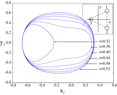
Fig. 1 shows a transition from localization to global oscillation, and this dynamics change can be explained by the stable point analysis. This reduced system is integrable as these equations satisfy two constants of motion;

$$\Omega(z_{1}+2z_{2})+\frac{3\chi Nx_{2}^{2}}{2} = H/N$$ (24)

$$3x_{2}^{2}+2(y_{2}^{2}+z_{2}^{2})+z_{1}^{2} = 4/3,$$ (25)

which correspond to energy and total number conservation respectively. The latter constant (25) follows from two stricter constraints

$$\left(\frac{2}{3}+x_{2}\right)^{2} = z_{1}^{2}$$ (26)

$$2\left(x_{2}+\frac{1}{6}\right)^{2}+y_{2}^{2}+z_{2}^{2} = \frac{1}{2},$$ (27)

which are derived from Eq. (5) with the symmetric condition in the semiclassical limit.

The equations of motion with the chosen initial conditions may be solved explicitly as a function of $x_{2}$ and depend on only one parameter; the ratio of the coupling constant $\Omega$ to the interaction strength $\chi$,

$$r=\frac{\Omega}{N\chi}\;(\geq 0).$$ (28)

The solutions are,

$$z_{1}(t) = x_{2}(t)+\frac{2}{3}$$ (29)

$$z_{2}(t) = -\frac{x_{2}(t)}{2}-\frac{3x_{2}(t)^{2}}{4r}+\left(-\frac{1}{3}+\frac{1}{3r}\right)$$ (30)

$$y_{2}(t)^{2} = f(x_{2}(t)),$$ (31)

where

$$f(x_{2}(t)) = -\left(a(r)-\left(x_{2}(t)+\frac{r}{3}\right)^{2}\frac{3}{4r}\right)^{2}$$ (32)

$$\;\;\;\;+\frac{2r}{3}\left(x_{2}(t)+\frac{r}{3}\right)(2-\frac{1}{r})+B(r),$$ (33)

and where the integration constants are given by

$$a(r) = -\frac{4r}{3}+\frac{(r-2)^{2}}{12r}$$ (34)

$$B(r) = \left(\frac{4r}{3}\right)^{2}-\frac{2}{9}(2r-1)(r-2).$$ (35)

The solutions are oscillatory and only exist for $-2/3\leq x_{2}\leq 1/3$, and are strongly dependent on the roots of the function $f(x)$. $f(x_{2})$ is fourth order in terms of $x_{2}$ and can have up to four real roots. For increasing $r$, the root structure of $f(x_{2})$ changes. To really understand these changes it is instructive to look at the fixed point structure of system (18). If all the derivatives of the equations of motion (18) are zero then,

$$y_{2}=0,$$ (36)

$$-3x_{2}-z_{1}+z_{2}+\frac{3}{r}z_{2}x_{2}=0.$$ (37)

Taking the positive root for $z_{1}$ in the constraint (27), $z_{1}=x_{2}+2/3$, the second equation can be written

$$-4x_{2}+z_{2}+\frac{3}{r}z_{2}x_{2}-\frac{2}{3}=0.$$ (38)

So the fixed points are the crossing points of this equation with the constraint,

$$2\left(x_{2}+\frac{1}{6}\right)^{2}+z_{2}^{2}=\frac{1}{2},$$ (39)

obtained by applying $y_{2}=0$ to constraint (27). Together these result in the following fourth order ploynomial in $z_{2}$

$$\frac{18}{r^{2}}\left(z_{2}-\frac{2}{3}\right)\left(z_{2}^{3}+\frac{2}{3}(1-4r)z_{2}^{2}-2r(1-r)z_{2}+\frac{4r^{2}}{3}\right)=0.$$ (40)

Fig. 2 shows the curves (38) and (39) in the $x_{2}$–$z_{2}$ plane for various values of $r$. The first factor of (40) gives us the point $A$ ($x=0,z_{2}=\frac{2}{3}$). For larger $r$ only one branch of the hyperbola (38) intersects the constraint and there are just two elliptic fixed points, one at A and one in the third quadrant. The solutions with initial condition $x_{2}=-\frac{2}{3}$ are far away from the elliptic fixed points and perform large delocalised oscillations on the sphere (27). A projection of one such solution is shown in Fig. 1 for $r=0.52$. As $r$ is decreased a second branch touches the constraint at C Fig. 2.

FIG. 2.: The $r$ dependence of the stable points. Each hyperbolic curve shows equation (38) for different $r$, while the ellipse represents constraint (39). Point $A$ is a stable point for any $r$. Point $B$ shows when the equation (38) collapses into the two lines, and point $C$ is the unique point of tangential contact to the ellipse.

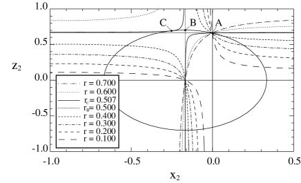
This occurs when the second factor in (40) has a double root at $r=0.507425$. Two new fixed points, a saddle and a center, then appear and move apart as $r$ is decreased away from $0.507425$. The stable and unstable manifolds of the saddle intersect, forming a lopsided figure eight like separatrix with the new elliptic fixed point in the one lobe and the elliptic fixed point at A in the other. When $r$ is $\frac{1}{2}$ the hyperbola reduces to the lines $z_{2}=\frac{2}{3},x_{2}=-\frac{1}{6}$ and the solutions in $(x_{2},y_{2})$ space are symmetrical about $x_{2}=-\frac{1}{6}$. If $r$ is further decreased the separatrix approaches our initial condition (22). At $r=\frac{1}{3}$ the initial condition actually lies on the separatrix. This occurs when the unstable fixed point lies on the solution curve (29), which amounts to looking for a double root of $f(x_{2})$. If we let $u=x_{2}+\frac{r}{3}$, then

$$f(u-\frac{r}{3})=-\left(a(r)-\frac{3u^{2}}{4r}\right)^{2}+\frac{2u}{3}(2r-1)+B(r).$$ (41)

and we require $f=0$ and $f^{\prime}=0$. $f^{\prime}=0$ gives,

$$u^{2}=\frac{4r}{9}\left(a(r)-\sqrt{4a(r)^{2}-3B(r)}\right),$$ (42)

which when substituted into $f=0$ gives only one real solution at $r_{*}=1/3$, $x_{2}=0$. Now for $r>\frac{1}{3}$ the solutions lie within the separatrix and so as $r$ is decreased through $\frac{1}{3}$ the oscillations suddenly reduce to half their former size as can be clearly seen in Fig. 1.

In the physical space of the potential then, the condensate remains localized at the bottom of the first well,$x_{2}=-\frac{2}{3}$, for $r=0$ . As we increase $r$ from zero, $x_{2}(t)$ begins to oscillate. In the $x_{2}-y_{2}$ plane, the point is replaced by small oscillations, within the separatrix, which pass through $x_{2}=-2/3$. This is referred to as dynamical localization. Even though the coupling between wells is present, the nonlinear interaction between particles prevents the condensate from moving away from its initially localized state. Eventually for the critical value of $r_{=}\frac{1}{3}$ the orbit in the $x_{2}-y_{2}$ plane extends across both half planes for positive and negative $x_{2}$ values and the condensate is no longer localized.

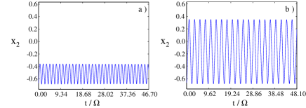
In Fig. 1 we show the phase space orbits of the semiclassical dynamics projected onto the $x_{2}-y_{2}$ plane for various values of the parameter $r$. The initial conditions correspond to a condensate localized in well 3. The transition from localized to delocalized motion is seen when the orbit in the phase space extends into the $x_{2}>0$ half of the plane. In Fig. 3 we plot $x_{2}(t)$ as a function of time for the condensate initially localized in well 3 with the same initial conditions as in Fig. 1 for two values of $r$, one above and below the critical value $r_{*}$ for localization. The transition from localized to delocalized oscillations is apparent.

FIG. 3.: Time evolution of $x_{2}(t)$ in the semiclassical regime versus time below (Figure a) and above (Figure b) the critical value $r_{*}=1/3$ for localization. Figure a) corresponds to the below threshold regime with $r=0.283$ while figure b) corresponds to the above threshold regime with $r=0.506$. The number of atoms is fixed at $N=50$, and the time $t$ is normalized by $\Omega$.

IV Quantum dynamics

In this section we treat the three coupled BEC model fully quantum mechanically and numerically calculate the time evolution of the particle distribution with the initial condition $|e_{1}\rangle$. For fixed total atom number $\hat{N}$, a suitable basis of the system Hilbert space is the number eigenstates $|n,m,N-(n+m)\rangle$ which are simultaneous eigenstates of the generators, $\hat{X}_{1}$ and $\hat{X}_{2}$ of the Abelian sub-algebra of SU(3). The unitary evolution operator is given by $U(t)=\exp\left[-iHt\right]$ where $H$ is specified by (11). The unitary evolution matrix is then computed and the initial state $|\psi(0)\rangle=|e_{1}\rangle$ is then propagated forward in time. At each time step we compute the averages of $\langle\hat{X}_{1}\rangle$ and $\langle\hat{X}_{2}\rangle$. These averages show the particle distribution projected on the y and x axes in Fig. 1 respectively. However because of the initial conditions for the state $|\psi(0)\rangle$ the average of $\langle\hat{X}_{1}\rangle$ does not change and in fact remains zero. It is not considered further here.

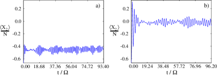
Fig. 4 shows the evolution of a condensate initially localized in state $|e_{1}\rangle$ with number of atoms fixed at $N=50$. For short times we see the same oscillations as in the corresponding semiclassical case, both below and above the critical value $r_{*}$. The oscillations of the quantum mean values decay due to the intrinsic quantum fluctuations in the number of atoms in each individual well, while the total particle number in the system remains fixed. The collapses and revivals of the oscillations in the quantum system arise from the discrete nature of the eigenvalue spectrum for finite atom number. Such phenomena were also observed in two coupled condensates [7].

FIG. 4.: The quantum dynamics of $\langle\hat{X}_{2}\rangle$ versus time below (Figure a) and above (Figure b) the critical value $r_{*}=1/3$ for localization. Figure a) corresponds to the below threshold regime with $r=0.283$ while figure b) corresponds to the above threshold regime with $r=0.506$. The number of atoms is fixed at $N=50$, and the time is normalized by $\Omega$.

One of the interesting higher dimensional features of this system is the existence of non-zero circular current states. For $r=0$, the system has the three-fold degenerate ground states, $|e_{1}\rangle$, $|e_{2}\rangle$, and $|e_{3}\rangle$, and superpositions of those states create another set of orthonormal ground states given as

$$|g_{1}\rangle = \frac{1}{\sqrt{3}}\left(|e_{1}\rangle+|e_{2}\rangle+|e_{3}\rangle\right)$$ (43)

$$|g_{2}\rangle = \frac{1}{\sqrt{3}}\left(e^{-i2\pi/3}|e_{1}\rangle+|e_{2}\rangle+e^{i2\pi/3}|e_{3}\rangle\right)$$ (44)

$$|g_{3}\rangle = \frac{1}{\sqrt{3}}\left(e^{-i2\pi/3}|e_{1}\rangle+e^{i2\pi/3}|e_{2}\rangle+|e_{3}\rangle\right).$$ (45)

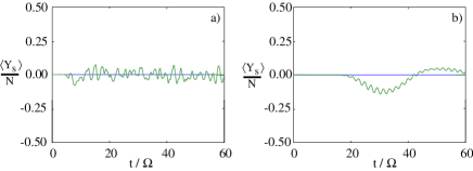
These states are invariant under $2\pi/3$ rotations due to system symmetries, as discussed in [16]. Taking the state $|g_{2}\rangle$, we examine the quantum dynamics of the angular momentum $\hat{Y}_{s}=\hat{Y}_{1}+\hat{Y}_{2}+\hat{Y}_{3}$. (The state $|g_{3}\rangle$ gives the same dynamics, however since these states are anti-symmetric to each other, clockwise motion in $|g_{2}\rangle$ corresponds anti-clockwise in $|g_{3}\rangle$.) For $r=0$, the state $|g_{2}\rangle$ is the ground state, and the average angular momentum remains zero, though for non-zero $r$, a non-zero average angular momentum appears as seen in Fig. 5. This shows quantum dynamics of the average angular momentum normalized by the total number $N$ for two different values of $r$. For small $r$ the non-zero angular momentum does not develop into any stable circular motion (Fig. 5a), while circular motion can be established for large $r$ (Fig. 5b), and becomes increasingly stable for larger $r$.

FIG. 5.: The quantum dynamics of $\langle\hat{Y}_{s}\rangle/N$ versus time with the initial state $|g_{2}\rangle$, where $\hat{Y}_{s}=\hat{Y}_{1}+\hat{Y}_{2}+\hat{Y}_{3}$ is the angular momentum. The angular momentum for small $r=0.5$ (Figure a) fluctuates, while non-zero circular motion appears in Figure b) for larger $r=1.3$. The number of atoms is fixed at $N=50$, and the time is normalized by $\Omega$.

V Discussion and Conclusion

In this paper we have shown how the generators of SU(3) can be used to describe the quantum and semiclassical dynamics of three symmetrically coupled atomic Bose-Einstein condensates. By taking expectation values of the Heisenberg equations of motion and factoring all higher order moments we can derive the semiclassical mean field equations. The nonlinear terms arising from hard collisions lead to a dynamical bifurcation in the semiclassical dynamics as the tunneling strength is increased, reflecting a transition from localized dynamics to tunneling currents. The $r$ dependence of the system is much more complicated than that found for two coupled BECs. The $r$ dependence of the stationary solutions in this paper constitutes only a small part of the total complexity of this system and only some of the higher dimensional effects. Our quantum treatment verified the dynamical transition found in the semiclassical analysis. This three coupled BEC model is the simplest model to have non-zero circular current states, and we have shown non-zero circular motion can appear given appropriate initial conditions.

The analysis of this paper focused on comparing the semiclassical dynamics with the evolution of quantum mean values. This restricted analysis naturally suggests further examination of the dynamics of full quantum states. However in order to examine full quantum states, it is necessary to use more powerful group theoretic tools and this will be the subject of a future paper.