Quantum Trajectories, Real, Surreal or an Approximation to a Deeper Process?

Abstract

The proposal that the one-parameter solutions of the real part of the Schrödinger equation (quantum Hamilton-Jacobi equation) can be regarded as ‘quantum particle trajectories’ has received considerable attention recently. Opinions as to their significance differ. Some argue that they do play a fundamental role as actual particle trajectories, others regard them as mere metaphysical appendages without any physical significance. Recent work has claimed that in some cases the Bohm approach gives results that disagree with those obtained from standard quantum mechanics and, in consequence, with experiment. Furthermore it is claimed that these trajectories have such unacceptable properties that they can only be considered as ‘surreal’. We re-examine these questions and show that the specific objections raised by Englert, Scully, Süssmann and Walther cannot be sustained. We also argue that contrary to their negative view, these trajectories can provide a deeper insight into quantum processes.

1 Introduction

The significance of the one-parameter solutions of the modified Hamilton-Jacobi equation of Bohm [1] has been the subject of many discussions over the years. (For more details of this approach see Bohm and Hiley [2] [3], Holland [4] and Dürr, Goldstein and Zanghi [5]) Attempts to explore these solutions and to give them physical significance in terms of particle trajectories has often been met with strong opposition. For some they are merely ‘metaphysical baggage’ with no real physical significance and should therefore not be pursued further (Pauli [6] and Zeh [7]). Relatively recently Englert, Scully, Süssmann and Walther [ESSW2] [8] and Scully [9] have claimed to show that these ‘trajectories’ lead to results that disagree with the standard interpretation of quantum mechanics. However their ‘standard’ interpretation is not the one that is usually called the Copenhagen interpretation. Furthermore they claim that these ‘trajectories’ have such bizarre properties that they cannot possibly be considered as ‘real’ particle trajectories and must be regarded as ‘surreal’, thus having no physical significance.

The specific conclusions of ESSW2 were answered by Dewdney et al [10] and by Dürr et al [11], who use the term Bohmian Mechanics to describe their own version of what was introduced by Bohm [1] and developed by Bohm and Hiley [2] [3]. However their answers have not removed the perceived difficulties as was shown in Englert et al [ESSW3] [12] and in a more recent paper Scully [9] repeats the criticisms contained in the earlier papers of ESSW2 and ESSW3.

In ESSW3 we find the statement that

Nowhere did we claim that BM makes predictions that differ from those of standard quantum mechanics.

Yet in ESSW2 we find

In other words: the Bohm trajectory is here macroscopically at variance with the actual, that is: observed, track.

Again in Scully [9] we find

These [Bohm] trajectories are not the ones we would expect from QM which predicts that atoms go along path 2 into detector A (our D₂) and along 1 into B (our D₁). (See figure 1 below).

Either the predictions are the same, in which case there is no reason to favour one approach over the other except for personal preferences, or the predictions are different in which case we can allow experiment to decide. We will see that no experiment can decide between the standard interpretation and the Bohm interpretation. The conclusions to the contrary that were claimed by ESSW2 involve adding an additional assumption to the standard theory that leads to an internal contradiction in their work.

The alleged difference arises from a consideration of the experiment shown in figure 1. If a measurement of the energy of the cavity after the particle is detected at D₂ is found to be in an excited state, ESSW2 conclude that “the atom must have actually gone through the cavity”. It is easy to show that not all the Bohm trajectories actually go through the cavity even though it is left in an excited state (see figure 5). Thus the two approaches appear to lead to contradictory results.

There is no disagreement about how the Bohm trajectories behave. The disagreement arises from the answer to question: “Is it correct, within orthodox quantum mechanics, to conclude that an atom must have actually gone through the cavity when we find it in an excited state after the atom has been detected in D₂?” We will discuss this question in detail in section 2 of this paper, but it should be noted that in order to reach this conclusion we must assume that it is only when a particle actually goes through such a detector that an exchange in energy is possible. This is an additional assumption that is not part of the interpretation proposed by Bohr and the Copenhagen school and is not part of standard quantum mechanics.

We will show that this assumption leads to the well-known contradiction that when interference effects are involved, we are obliged to say that, on the one hand, the atom always chooses one of the two ways, but behaves as if it had passed both ways [13]. If our objections are correct then the Bohm trajectories cannot be ruled out by the arguments presented in ESSW2.

Further objections to the Bohm approach have been made by Aharonov and Vaidman [14] and by Griffiths [15]. Unfortunately, in the case of Aharonov and Vaidman [14], they have not used the approach introduced by Bohm [1] and further developed in Bohm and Hiley [2] [3]. In their own words “The fact that we see these difficulties follow from our [AV] particular approach to the Bohm theory in which the wave is not considered to be a ‘reality’.” [14]

The basic assumptions used in Bohm and Hiley [3] are set out in their book, The Undivided Universe. Assumption 1 defines the role played by the particle and is the same as assumption 1 in Aharonov and Vaidman, but assumption 2 reads “This particle is never separate from a new type of field that fundamentally affects it. This field is given by $R$ and $S$ or alternatively by $\psi=R\mbox{ exp}(iS/\hbar)$. $\psi$ satisfies the Schrödinger equation (rather than, for example, Maxwell’s equation), so that it too changes continuously and is causally determined.” Aharonov and Vaidman have replaced this last assumption by one that does not give the wave function the same role and, as a consequence, their criticisms do not apply to the Bohm approach we discuss in this paper. Nevertheless they have raised an interesting question concerning tracks produced in a bubble chamber, which we will address in section 5.5.

Our assumption 2 is the source of a number of features of quantum processes that, for one reason or another have been regarded as undesirable or unacceptable, “quantum non-locality” or “quantum non-separability”, being, perhaps, the most contentious. This feature clearly arises in our approach and was used by Dewdney et al [10] to explain the ‘strange’ behaviour of the trajectories. It seems that this non-local or non-separable feature disturbs ESSW3 because they write

It is quite unnecessary, and indeed dangerous, to attribute any additional “real” meaning to the $\psi$-function.

Unfortunately the specific ‘dangers’ are not spelt out.

The opposition to non-separability is deeply entrenched in spite of all that Bohr has written about quantum theory. He constantly emphasised that the central feature of quantum theory lay in the “impossibility of making a sharp separation between the behaviour of atomic objects and the interaction with the measuring instruments, which serve to define conditions under which the phenomena appear.”[16] Indeed as one of us has pointed out already [17], Bohr’s answer to the original Einstein-Podolsky-Rosen [18] objection depends on the ‘wholeness of the experimental situation’ which characterises the impossibility of making this sharp separation. In this regard the Bohm approach actually supports Bohr’s conclusions, although from a point of view that Bohr himself thought to be impossible! Thus we find it very strange that the reason for rejecting the Bohm approach is central to Bohr’s answer to the EPR objection and therefore, it to must be rejected.

Unfortunately the confusion we find in this field is not helped by the dogmatism that has become fashionable on both sides. These positions arise from what appear to be deeply held convictions as to what quantum physics ought to be rather than let experiment, mathematics and clear logic lead the debate. (After all both standard quantum mechanics and the Bohm approach claim to use exactly the same mathematics and to predict exactly the same experimental verifiable probabilities.) This dogmatism has generated much confusion over the role of ‘particle’ trajectories in quantum mechanics.

In this paper we will review the general situation and attempt to clarify how and where the disagreements arise. We hope that this discussion will be received in the spirit that it is written, namely it is an attempt to reach common ground in which both sides can actually agree on what are the essential differences. It is important to find out whether they are factual and amenable to experimental clarification or whether they are merely disagreements about what satisfies our demands for “common sense” theories.

2 Appraisal of arguments presented by Englert, Scully, Süssmann, Walther.

2.1 The general grounds.

Let us begin by considering some comments made in the recent paper by Scully [9]. He asks the specific question

Do Bohm trajectories always provide a trustworthy physical picture of particle motion?

and immediately provides the answer “No”, followed by the explanation

When particles detectors are included particles do not follow the Bohm trajectories as we would expect from a classical type model.

Unfortunately this critical sentence is not very clear. Is it saying that we somehow know which trajectories a particle would follow in the interferometer in question, or is it simply saying that the trajectories are not doing what we would expect from the point of view of classical physics?

If it is the latter, it is surely clear by now that we cannot explain quantum processes using classical physics, so why would we expect classical-type trajectories to account for quantum processes? If this is what is meant then the objection is not serious and can be dismissed immediately.

If, however, it is the former, then it implies that we know, independently of the Bohm approach, which trajectories the particles actually follow in an interferometer. Later in the same paper we find a much clearer statement confirming this view, which we have quoted above but which we will repeat again.

These [Bohm] trajectories are not the ones we would expect from QM which predicts that atoms go along path 2 into detector A [our D₂] and along 1 into B [our D₁].

But how do we know what trajectories the particles actually follow in orthodox quantum mechanics? Is it not an essential feature of standard quantum mechanics that when we are discussing interference or diffraction effects, talking about trajectories will lead to contradictions? For example, in discussing electron diffraction, Landau and Lifshitz [19] point out that since the interference pattern does not correspond to the sum of patterns given by each slit (beam) separately, “It is clear that this result can in no way be reconciled with the idea that electrons move in paths”.

Again Bohr [20], referring to an interferometer using photons rather than atoms, remarks:

In any attempt of a pictorial representation of the behaviour of the photon we would, thus, meet with the difficulty: to be obliged to say, on the one hand, that the photon always chooses one of the two ways and, on the other hand, [when the beams overlap] that it behaves as if it had passed both ways. It is just arguments of this kind which recall the impossibility of subdividing quantum phenomena and reveal the ambiguity in ascribing customary physical attributes to atomic objects.

He goes on to say that

all unambiguous use of space-time concepts in the description of atomic phenomena is confined to the recording of observations which refer to marks on a photographic plate or to similar practically irreversible amplification effects like building of a drop of water around an ion in a cloud-chamber.

On what grounds then is the claim that, in standard quantum mechanics, we can ‘know’ the path a particle takes as it passes through an interferometer being made? It is essential to get a clear answer to this question because without it, the rejection of Bohm trajectories on the grounds that it disagrees with quantum mechanics cannot be sustained. How then are trajectories to be determined in standard quantum mechanics?

The experiment central to this discussion is the interferometer sketched in figure 1

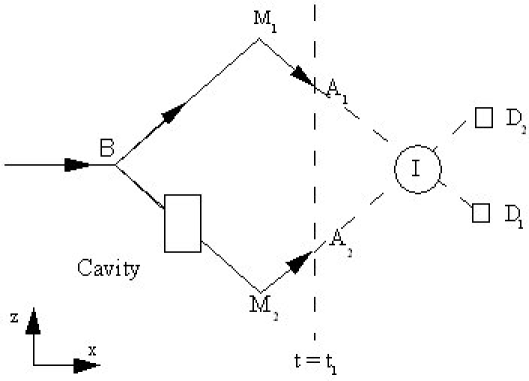
Figure 1: The interferometer considered by Scully [9].

A beam of atoms is incident on a beam-splitter B. Each atom is assumed to be in an excited (Rydberg) state. It is further assumed that each atom can be represented by a Gaussian wave packet of small width so that after passing through the beam-splitter, B, the wave packets follow the two paths $BM_{1}A_{1}$ and $BM_{2}A_{2}$ and do not overlap again until they reach the region $I$.

Before reaching this region, a special cavity micromaser is placed in one of the arms of the interferometer as shown in figure 1. The aim of introducing this cavity is to provide a Welcher Weg (WW) device, which we can use to enable us to infer the path the atom took in passing through the interferometer.

The cavity has the essential property that when an excited atom is passed through it, the excitation energy is exchanged with the cavity, and the atom then continues in the same direction with the same momentum, but in a lower internal energy state. This means that when the cavity is part of an interferometer as shown in figure 1, the exchange of energy does not destroy the coherence between the two beams.

It is then claimed that, by measuring the energy in the cavity after the atom has passed through the interference region $I$, we will be able to infer along which arm the atom actually went. If this claim is correct then not only does it rule out the Bohm approach, it also throws doubts on the validity of the assertions made by Landau and Lifshitz and by Bohr in the quotations presented above. The crucial question then is whether the cavity used in this way can give reliable information as to which path the atom actually took.

To answer this, it is crucial to analyse carefully how the cavity and the atom exchange energy, as it is this exchange process that lies at the heart of the objections raised by ESSW2 and Scully [9]. Our analysis will involve taking a careful look at what assumptions these authors make when they refer to ‘the standard approach to quantum mechanics.’

One primary assumption made in ESSW3 is that the wave function is merely a “tool used by theoreticians to arrive at probabilistic predictions.” This means that we must first analyse the interaction between the cavity and the atom classically so that a suitable interaction Hamiltonian can be written down. This Hamiltonian is then written in an operator form so that we can use the Schrödinger equation to solve for the time development of the wave function. Thus as far as quantum formalism is concerned, the interaction involves a change of relationship between the wave function of the atom and the wave function of the cavity. The quantum formalism does not require any knowledge of the position of the atom. The formalism enables us to calculate the probability of finding an atom at any given point at any given time.

Since the interaction Hamiltonian is local and the atom is represented by a Gaussian wave packet of narrow width, the corresponding ket for the whole system at time $t=t_{1}$ (See figure 1) is

$$|\Psi(t=t_{1})\rangle=|\psi_{1}\rangle|\Phi_{0}\rangle+|\psi_{2}\rangle|\Phi_{E}\rangle$$ (1)

where $|\psi_{1}\rangle(|\psi_{2}\rangle)$ is the ket of the excited (unexcited) atom and $|\Phi_{0}\rangle(|\Phi_{E}\rangle)$ is the ket of the unexcited (excited) cavity. In writing down this expression we are assuming that no irreversible process takes place when the cavity is added. In terms of wave packets, we can write $\psi_{1}(\mathbf{r}_{a})\phi_{1}(\mathbf{\eta}_{a})=\langle\mathbf{r}_{a},\mathbf{\eta}_{a}|\psi_{1}\rangle$ and $\psi_{2}(\mathbf{r}_{a})\phi_{2}(\mathbf{\eta}_{a})=\langle\mathbf{r}_{a},\mathbf{\eta}_{a}|\psi_{2}\rangle$ where $\psi$ is the wave function of the centre of mass of the atom with centre of mass co-ordinates $\mathbf{r}_{a}$ and $\phi$ in the internal wave function depending on the variables $\mathbf{\eta}_{a}$.

After the wave packets have separated, they do not overlap prior to $t=t_{1}$, so we can talk about ‘the wave packet $\psi_{1}(\mathbf{r}_{a}$) travelling along the path BM₁A₁’ and ‘the wave packet $\psi_{2}(\mathbf{r}_{a}$) travelling along BM₂A₂’. At this stage we can associate an atom with a particular wave packet and talk about the ‘atom travelling along BM${}_{1}A_{1}$’ or ‘along BM₂A₂’ without running into any difficulties.

However once the packets overlap again as they enter the region $I$, we must proceed with caution, particularly in view of the warnings given by Bohr [13] and Landau and Lifshitz [19] in the quotations above. The key objection they raise is that if we give relevance to the atom as opposed to the wave function, we are forced to say that the atom always chooses one path, but behaves as if it had passed both ways. How has this objection been avoided in ESSW2?

Let us concentrate on the region of overlap $I$. We have argued that the interaction with the cavity does not destroy the coherence between the two beams when they subsequently overlap again. This means that the beam can be legitimately described by the ket $|\Psi\rangle$ given by equation (1). However if the interaction were to destroy the coherence, then we must replace this ket by the density operator

$$\rho=|\psi_{1}\rangle|\Phi_{0}\rangle\langle\psi_{1}|\langle\Phi_{0}|+|\psi_{2}\rangle|\Phi_{E}\rangle\langle\psi_{2}|\langle\Phi_{E}|$$ (2)

This would describe two separate wave packets moving through the region $I$ without interfering with each other. In other words when an atom enters the beam BM₁A₁, it is confined to the packet $\psi_{1}$ which then moves along the path BM₁A₁ and continues without deviation through the region $I$, finally arriving at D₁. An atom following the path BM₂A₂ will be in the wave packet $\psi_{2}$ and it too will continue also without deviation through the region $I$ until it is registered at D₂.

In this case there is no doubt that the atom actually follows one or other of the paths and that the atom that went through the cavity exchanged energy with it and then continued on to D₂. There is no problem here

2.2 The region of coherent overlap.

The case that does present difficulties is the one that arises only when coherence is maintained. Here the correct description of the experimental set-up is provided by the ket $|\Psi\rangle$. Let us consider the situation at a time $t=t_{3}$, after the atom has passed through the region $I$ so that there is no longer any overlap between the two wave packets. The experimental predictions are quite clear. If D₁ fires, we will find the cavity is unexcited, whereas if D₂ fires, the cavity will be found to be excited.

This conclusion is reached in both interpretations. No assumptions about possible particle trajectories are needed to arrive at this conclusion. Clearly this result is quite consistent with the statement ‘the atom passed through the cavity on its way detector D₂’. However consistency does not mean that the atom did actually go through the cavity.

The key question then is “How can we show which way the atom reaching D₁ or D₂ actually went in either case?” ESSW3 claim that we can do this within the framework of standard quantum mechanics and it is the presence of the cavity that enables us to talk about “the detected, actual way through the interferometer.” This is the key statement upon which ESSW base all their conclusions and it must be examined very carefully.

The first point to notice is that the cavity, which ESSW are regarding as a ‘measuring’ device, does not function in the same way as a traditional measuring device in standard quantum mechanics. The cavity is a quantum system and no irreversible mark has been left in any system. Since it leaves no irreversible mark, it is not a measuring device in the traditional sense as defined by Bohr (See quotation above). ESSW claim that the cavity gives us a new type of measurement, which does not leave a permanent record and can be easily ‘erased’[24]. Thus ESSW are talking about an aspect of quantum mechanics that is not contained in the Copenhagen interpretation.

In order to emphasise the difference, let us look more carefully at orthodox measurement. To discuss a measurement Bohr introduces the word ‘phenomenon’ defined in the following way:

As a more appropriate way of expression I advocate the application of the word phenomenon exclusively to refer to the observations obtained under specified circumstances, including an account of the whole experimental arrangement [25].

But we must take it further. As Wheeler [26] puts it: “No elementary quantum phenomenon is a phenomenon until, in the words of Bohr [27] ‘It has been brought to a close’ by ‘an irreversible act of amplification’”. In drawing attention to this traditional thinking we are not, at this stage making any value judgements. We are simply drawing attention to the fact that ESSW have added something new to what we would call ‘standard quantum mechanics’.

The key assumption used by ESSW is that energy exchange only takes place when the actual atom interacts locally with the photon field in the cavity. This does not merely mean that the interaction Hamiltonian is local, but that the interaction can take place if and only if the atom is physically present in the cavity. This is a new assumption that is not part of standard quantum mechanics and certainly not part the Bohr (Copenhagen) interpretation.

Given this new assumption, the question that we must examine is: “Can we give a consistent account of quantum interference phenomena without running into the difficulties pointed out by Bohr and by Landau and Lifshitz above?”

As we will be interested in the region of interference $I$ in figure 1, let us insert a horizontal beam-splitter at $I$. This turns the experimental set-up into a Mach-Zender interferometer, which will enable us to demonstrate unambiguously the interference properties that occur in region $I$.

Without the cavity in the arm BM₂A₂, we find for the symmetrical set-up that all the atoms end up in D₂. If we now include the cavity in the arm BM₂A₂, we find the probability for D₁ firing is given by the expression

$$P(D_{1})=1/4[\langle\psi_{1}|\psi_{1}\rangle\langle\Phi_{0}|\Phi_{0}\rangle+\langle\psi_{2}|\psi_{2}\rangle\langle\Phi_{E}|\Phi_{E}\rangle$$

$$+\langle\psi_{1}|\psi_{2}\rangle\langle\Phi_{0}|\Phi_{E}\rangle+\langle\psi_{2}|\psi_{1}\rangle\langle\Phi_{E}|\Phi_{0}\rangle]$$ (3)

While the probability for $D_{2}$ firing is

$$P(D_{2})=1/4[\langle\psi_{1}|\psi_{1}\rangle\langle\Phi_{0}|\Phi_{0}\rangle+\langle\psi_{2}|\psi_{2}\rangle\langle\Phi_{E}|\Phi_{E}\rangle$$

$$-\langle\psi_{1}|\psi_{2}\rangle\langle\Phi_{0}|\Phi_{E}\rangle-\langle\psi_{2}|\psi_{1}\rangle\langle\Phi_{E}|\Phi_{0}\rangle]$$ (4)

We see that we get a new firing probability for the detectors depending on whether (a) $|\psi_{1}\rangle$ is orthogonal to $|\psi_{2}\rangle$, (b) $|\Phi_{0}\rangle$ is orthogonal to $|\Phi_{E}\rangle$ or (c) both (a) and (b).

All of this is very obvious and straight forward, but now the assumption that ESSW make is that the atom must have actually gone through the detector to exchange energy. ESSW3 write:

-the interpretation of the Bohm trajectory – is implausible, because this trajectory can be macroscopically at variance with the detected, actual way through the interferometer. And yes, we do have a framework to talk about path detection; it is based upon the local interaction of the atom with the photons inside the resonator, described by standard quantum theory with its short range interactions only.

Thus the claim is that the only way that the cavity can be excited is if the atom actually passes through it. This means that with the cavity in place 50% of the atoms actually go through the cavity and end up triggering D₂. The remaining 50% actually pass down the other arm and end up triggering D₁.

However when the cavity is removed, all the particles end up in $D_{2}$. How then does one explain why the particles travelling down BM₁A₁ stop travelling on to $D_{1}$ and instead travel to $D_{2}$? Nothing has been changed in path $1$ yet somehow the particles travelling along path $1$ ‘know’ the cavity is present in path $2$ or not as the case may be?

Recall that ESSW insist that only short range interactions are allowed in standard quantum mechanics. There is no explanation of this change of behaviour and we are simply left with the contradiction that Bohr[20], and Landau and Lifshitz[19] have already pointed out, namely, that “the photon always choose one of two ways” but “behaves as if it had passed both ways.”

The above results indicate that coherence is maintained and the absence of interference should not be taken to mean a loss of coherence between the two beams in the region I. These two beams must be treated as remaining coherent. This would certainly not be the case if we measured the energy in the cavity before the atom reached the region I. But that would require an irreversible process to occur in the recording of the result. In that case, in Wheeler’s terms “the phenomenon is complete” and we have information that will enable us to say along which path the atom actually travelled. Mathematically this would mean replacing the wave function (1) by the density operator (2).

It might be argued that it is the exchange of energy that is responsible for the lack of interference or ‘decoherence’. However this cannot be true. If we add any device that interacts with the atom, energy must be exchanged even if this energy induces only a change of phase. This would occur if the atom were to interact with an oscillator in a coherent state. Since coherent states are not orthogonal, the interference does not disappear, showing that merely an exchange of energy is NOT responsible for decoherence.

2.3 How the Copenhagen interpretation deals with this situation.

The traditional way to avoid all of these difficulties is to give up any attempt to follow a particle along a well-defined path, particularly in an interferometer. This does not mean that we can never talk about the path of a particle. Heisenberg [21] pointed out in 1927 that before we can talk about a path, we have to be clear as to what is to be understood by the words “position of the object”. He writes

When one wants to be clear about what is to be understood by the words “position of the object”, for example of the electron, then one must specify experiments with which whose help one plans to measure the “position of the electron”; otherwise this word has no meaning.

Conventional measurement requires the observable to be represented by an operator and after the measurement is complete, the particle is left in an eigenstate of the operator. ESSW2 specifically rule out any change of the centre-of-mass motion and therefore the atom is not in a position eigenstate after it leaves the cavity. Nor is it a ‘detection’ in the same sense as when the atom is recorded at D₁ or D₂. Here some form of irreversible amplification involved. Rather their notion of measurement involves inference based on the assumption that energy exchange can only take place when the atom is physically present in the cavity.

There is no difficulty here if the energy of the cavity is measured before the atom reaches $I$. However if we leave this measurement until after the atom has passed through $I$, the wave functions obtained from equation (1) shows that there is a coupling between $\psi_{1}(\mathbf{r}_{a})$ and $\psi_{2}(\mathbf{r}_{a})$. Bohr and Wheeler argue that this coupling cannot be ignored until the whole process is “brought to a close by an irreversible act of amplification”. If we do ignore the coupling and follow ESSW we are led to the contradiction that “although the particle travels down one path of an interferometer, it behaves as if it went down both paths.”

This is just what the Copenhagen interpretation warns us about. To emphasise this point again, consider the following quotation taken from Bohr [22]:

In particular, it must be realised that - besides in the account of the placing and timing on the instruments forming the experimental arrangement - all unambiguous use of space-time concepts in the description of atomic phenomena is the recording of observations which refer to marks on a photographic or similar practically irreversible amplification effects like the building of a water drop around an ion in a cloud-chamber.

Thus the storage of a single quantum of energy in the cavity does not constitute a measurement. There is no ‘irreversible amplification’ until the atom is detected in D₁ or D₂.

As we have already remarked above, if we measure the energy in the cavity after the atom passes through the cavity but before it reaches the region $I$, an irreversible change does take place and the coherence between the two beams is subsequently destroyed. In this case we must use the density operator (2) in the region $I$ and then we can unambiguously conclude that the atom passed through the cavity and its energy can be used to infer that the atom passed through the cavity. But once we allow the beams to intersect in the region $I$, we can no longer make this inference without making the assumption that leads to the contradiction discussed above. This is why Heisenberg [23] wrote:

If we want to describe what happens in an atomic event, we have to realise that the word ‘happens’ can only apply to observations, not to the state of affairs between two observations.

The notion of a WW device has no meaning whatsoever in the Copenhagen interpretation and we cannot use it to give a meaning to which way the particle passed through the interferometer. The inference that the energy in the cavity can reveal what path the atom took is incorrect once the atom has entered the region $I$ and as a consequence the claim that one can use quantum mechanics to show that the Bohm trajectories are “meaningless” cannot be sustained.

3 Probability currents

One of the features of the Bohm theory that generates misgivings is the fact that it predicts that atoms do not cross the $z=0$ plane of symmetry when there is no cavity in either arm (see figure 3). This result has been greeted with surprise, if not disbelief. How is it possible for atoms to be so drastically deflected when there appears to be nothing in the region $I$ that could bring about this reflection? Before answering this question from the Bohm perspective, let us first see if there is anything within the orthodox interpretation that might enable us to find some way of exploring what might be going on the region $I$.

Central to standard quantum mechanics is probability and its conservation as expressed through the equation

$$\frac{\partial P}{\partial t}+\nabla.{\mathbf{j}}=0$$ (5)

In order to conserve probability as a local probability density we need to interpret $\mathbf{j}$ as probability current. It is in this way that orthodox quantum mechanics allows us to talk meaningfully about probability currents.

Indeed these currents are used extensively in many branches of quantum physics including scattering theory, condensed matter physics and superconductivity, where we can discuss the flow of charge across boundaries. We can interpret these currents without changing the significance of the wave function, which can still be regarded as a ‘tool’, forming part of an algorithm. It is this algorithm that enables us calculate not only probabilities, but also probability currents in any given experimental set-up. Could these probability currents supply further information about the flux of atoms in the region of interference, $I$, and hence about the flux across the $z=0$ plane?

It is interesting to note that ESSW2 actually use these currents to criticise the Bohm interpretation, attributing their properties to the Bohm interpretation and do not seem to realise that the probability currents are part of the orthodox quantum mechanics

Let us first use the probability currents to explore the difference between the situation described by the ket $|\Psi\rangle$ given by equation (1) and the density operator $\rho$ given by equation (2).

The probability current is defined by

$$\mathbf{j}=\frac{\hbar^{2}}{2mi}[\Psi^{*}(\nabla\Psi)-(\nabla\Psi^{*})\Psi]$$ (6)

In the case of the density operator each term gives rise to an independent current, $\mathbf{j}_{1}$ and $\mathbf{j}_{2}$, where

$$\mathbf{j}_{i}=\frac{\hbar^{2}}{2mi}[\Psi_{i}^{*}(\nabla\Psi_{i})-(\nabla\Psi_{i}^{*})\Psi_{i}]\hskip 28.45274pt(i=1,2)$$ (7)

These latter currents cross the region $I$ from A₁ to D₁ and from A₂ to D₂ respectively. In other words the currents do not ‘see’ each other and there is no ambiguity as to what is happening in this case. Indeed the consideration of the probability currents merely confirms our previous discussion.

Let us now turn to consider what happens in the situation described by the ket $|\Psi\rangle$. We first consider the case when no cavity is present in either arm of the interferometer. Here the wave function is simply

$$\Psi_{I}(\mathbf{r}_{a})=\psi_{1}(\mathbf{r}_{a})+\psi_{2}(\mathbf{r}_{a})$$ (8)

The probability current for the atoms in the region of overlap $I$, is given by

$$\mathbf{j}(\mathbf{r}_{a})=\frac{\hbar^{2}}{2mi}[\psi_{1}^{*}(\mathbf{r}_{a})\nabla\psi_{1}(\mathbf{r}_{a})-\psi_{1}(\mathbf{r}_{a})\nabla\psi_{1}^{*}(\mathbf{r}_{a})]+[\psi_{2}^{*}(\mathbf{r}_{a})\nabla\psi_{2}(\mathbf{r}_{a})-\psi_{2}(\mathbf{r}_{a})\nabla\psi_{2}^{*}(\mathbf{r}_{a})]$$

$$+[\psi_{2}^{*}(\mathbf{r}_{a})\nabla\psi_{1}(\mathbf{r}_{a})-\psi_{1}(\mathbf{r}_{a})\nabla\psi_{2}^{*}(\mathbf{r}_{a})]+[\psi_{1}^{*}(\mathbf{r}_{a})\nabla\psi_{2}(\mathbf{r}_{a})-\psi_{2}(\mathbf{r}_{a})\nabla\psi_{1}^{*}(\mathbf{r}_{a})]$$ (9)

The first two terms in this expression are exactly the currents $\mathbf{j}_{1}$ and $\mathbf{j}_{2}$ calculated using the density operator

$$\rho=|\psi_{1}\rangle\langle\psi_{1}|+|\psi_{2}\rangle\langle\psi_{2}|$$ (10)

The third and forth terms correspond to the interference terms.

We could deal with this numerically and calculate the probability current in detail, but our main point can be made using the same argument employed by ESSW2. This depends on the fact that $\psi_{1}(\mathbf{r}_{a})$ is the reflected image of $\psi_{2}(\mathbf{r}_{a})$ about the horizontal line of symmetry ($z=0$) in figure 1. This means that

$$\psi_{1}(x,y,z,t)=\psi_{2}(x,y,-z,t)$$ (11)

In consequence the $x$- and $y$-components of the current vector is an even function in $z$, while the $z$-component is odd. Therefore the $z$-component of the current is an odd function of $z$, so that $j_{z}=0$ at $z=0$. Thus there is no probability current flowing across the horizontal plane, and hence no net particle-flux across this plane.

This could imply either (a) that no particles actually cross the $z=0$ plane, or (b) that the average particle flux crossing the plane is zero. But (b) is exactly the same as the result of using the density operator (9) when we simply add the two independent currents together. Clearly in this case there are as many particles travelling in the negative $z$-direction as there are crossing in the positive $z$-direction.

This could well be the case when we use the wave function (7) but now we cannot split the ensemble into two separate sub-ensembles because of the presence of observable interference effects. Therefore we cannot be sure that zero current arises because there are as many atoms crossing the $z=0$ plane one way as the other. Thus at best we are left with an ambiguity of being unable to decide between the two choices (a) and (b), but we certainly cannot rule out possibility (a) within quantum mechanics.

In order to explore the nature of this ambiguity further, let us consider a more general case when an energy-exchanging device, d_e-e is placed in one of the arms. We will again assume this device is a single state microscopic quantum system of some kind that does not introduce any irreversible effects. This could be, for example, a harmonic oscillator in an energy eigenstate, an oscillator in a coherent state, or some other form of phase shifter. It could even be an idealised system such as ‘particle in an infinite well’ (i.e. a particle in a ‘box’.) But no matter what the device is, we assume that some energy will be exchanged between the device and the atom.

Consider the case when the atom leaves the device d_e-e in an excited state that is not orthogonal to its ground state (for example, in a harmonic oscillator in a coherent state). Let the normalised wave function of this device before the interaction be $\eta_{0}(\mathbf{r}_{b}$) and after the interaction be $\eta_{1}(\mathbf{r}_{b}$). Here $\mathbf{r}_{b}$ is the position of the particle comprising the harmonic oscillator. Assuming coherence is not destroyed in the region I, the wave function at $t>t_{1}$ will be

$$\Psi_{1}(\mathbf{r}_{a},\mathbf{r}_{b})=\psi_{1}(\mathbf{r}_{a})\eta_{0}(\mathbf{r}_{b})+\psi_{2}(\mathbf{r}_{a})\eta_{1}(\mathbf{r}_{b})$$ (12)

We can form $|\Psi_{1}(\mathbf{r}_{a},\mathbf{r}_{b})|^{2}$ and integrate over $\mathbf{r}_{b}$ to obtain an expression for the probability of finding an atom at a particular point $\mathbf{r}_{a}$ in the region $I$. This is

$$P(\mathbf{r}_{a})=|\psi_{1}|^{2}+|\psi_{2}|^{2}+\alpha\psi_{1}^{*}\psi_{2}+\alpha^{*}\psi_{1}\psi_{2}^{*}$$ (13)

where $\alpha=\int\eta_{0}^{*}\eta_{1}d^{3}\mathbf{r}_{b}$.

It is clear from this expression that interference effects will be seen in the region $I$ along any $x=constant$ plane as long as $\alpha\neq 0$ (see figure 1). Let us see what effect this interference has on the probability currents.

In this case the conservation of probability is expressed through

$$\frac{\partial P(\mathbf{r}_{a},\mathbf{r}_{b})}{\partial t}+\nabla_{a}.\mathbf{j}_{a}({\mathbf{r}_{a},\mathbf{r}_{b}})+\nabla_{b}.\mathbf{j}_{b}({\mathbf{r}_{a},\mathbf{r}_{b}})=0$$ (14)

Here we have two currents, the first is the probability current for the atoms, which is given by

$$\mathbf{j}_{a}(\mathbf{r}_{a},\mathbf{r}_{b})=\frac{\hbar^{2}}{2mi}\{[\psi_{1}^{*}(\mathbf{r}_{a})\nabla_{\mathbf{r}_{a}}\psi_{1}(\mathbf{r}_{a})-\psi_{1}(\mathbf{r}_{a})\nabla_{\mathbf{r}_{a}}\psi_{1}^{*}(\mathbf{r}_{a})]|\eta_{0}(\mathbf{r}_{b})|^{2}$$

$$+[\psi_{2}^{*}(\mathbf{r}_{a})\nabla_{\mathbf{r}_{a}}\psi_{2}(\mathbf{r}_{a})-\psi_{2}(\mathbf{r}_{a})\nabla_{\mathbf{r}_{a}}\psi_{2}^{*}(\mathbf{r}_{a})]|\eta_{1}(\mathbf{r}_{b})|^{2}$$

$$+[\psi_{2}^{*}(\mathbf{r}_{a})\nabla_{\mathbf{r}_{a}}\psi_{1}(\mathbf{r}_{a})-\psi_{1}(\mathbf{r}_{a})\nabla_{\mathbf{r}_{a}}\psi_{2}^{*}(\mathbf{r}_{a})]\eta_{0}(\mathbf{r}_{b})\eta_{1}^{*}(\mathbf{r}_{b})$$

$$+[\psi_{1}^{*}(\mathbf{r}_{a})\nabla_{\mathbf{r}_{a}}\psi_{2}(\mathbf{r}_{a})-\psi_{2}(\mathbf{r}_{a})\nabla_{\mathbf{r}_{a}}\psi_{1}^{*}(\mathbf{r}_{a})]\eta_{0}^{*}(\mathbf{r}_{b})\eta_{1}(\mathbf{r}_{b})\}$$ (15)

Notice this current is a function of both $\mathbf{r}_{a}$ and $\mathbf{r}_{b}$, showing that it is in configuration space. For local measurements we must find this current as a function of $\mathbf{r}_{a}$ alone, and therefore we must integrate over all $\mathbf{r}_{b}$. If the wave functions, $\eta_{0}(\mathbf{r}_{b})$ and $\eta_{1}(\mathbf{r}_{b})$, are normalised, but not orthogonal, the probability current for the atoms is

$$\mathbf{j}_{a}(\mathbf{r}_{a})=\frac{\hbar^{2}}{2mi}\{[\psi_{1}^{*}(\mathbf{r}_{a})\nabla_{\mathbf{r}_{a}}\psi_{1}(\mathbf{r}_{a})-\psi_{1}(\mathbf{r}_{a})\nabla_{\mathbf{r}_{a}}\psi_{1}^{*}(\mathbf{r}_{a})]$$

$$+[\psi_{2}^{*}(\mathbf{r}_{a})\nabla_{\mathbf{r}_{a}}\psi_{2}(\mathbf{r}_{a})-\psi_{2}(\mathbf{r}_{a})\nabla_{\mathbf{r}_{a}}\psi_{2}^{*}(\mathbf{r}_{a})]$$

$$+\alpha[\psi_{2}^{*}(\mathbf{r}_{a})\nabla_{\mathbf{r}_{a}}\psi_{1}(\mathbf{r}_{a})-\psi_{1}(\mathbf{r}_{a})\nabla_{\mathbf{r}_{a}}\psi_{2}^{*}(\mathbf{r}_{a})]$$

$$+\alpha_{*}[\psi_{1}^{*}(\mathbf{r}_{a})\nabla_{\mathbf{r}_{a}}\psi_{2}(\mathbf{r}_{a})-\psi_{2}(\mathbf{r}_{a})\nabla_{\mathbf{r}_{a}}\psi_{1}^{*}(\mathbf{r}_{a})]$$ (16)

Clearly if $\alpha\neq\alpha^{*}$, $j_{z}$ is not an odd function of $z$ and therefore there is now a non-zero probability current crossing the $z=0$ plane. This probability current approaches zero as either $\alpha\rightarrow\alpha^{*}$,or when the wave functions of the added device are orthogonal ($\alpha=0$).

What we have shown here is that by following the standard approach, there is no probability current crossing the $z=0$ plane when there is no device in either beam. If we include some device in which the wave functions $\eta_{1}(\mathbf{r}_{b})$ and $\eta_{0}(\mathbf{r}_{b})$ are not orthogonal, then a current must cross the $z=0$ plane. Thus interference effects produce changes in the probability flux of the atoms.

However when these two wave functions are orthogonal, as in the case of the cavity then again there is no net current crossing the plane. We repeat again, although we cannot conclude from this that no atoms actually cross this plane, we cannot rule out this possibility. In the next section we will show that the Bohm trajectories do not cross the $z=0$ plane in this case showing that these trajectories are certainly consistent with standard quantum mechanics and therefore cannot be ruled out on these grounds.

The conservation equation contains a second probability current $j_{b}({\mathbf{r}_{a},\mathbf{r}_{b}})$ This current is for the device-particle $\mathbf{r}_{b}$. The wave functions for this device are $\eta_{0}(\mathbf{r}_{b})$ and $\eta_{1}(\mathbf{r}_{b})$. In this case the current would be

$$\mathbf{j}_{b}(\mathbf{r}_{a},\mathbf{r}_{b})=\frac{\hbar^{2}}{2mi}\{[\eta_{0}^{*}(\mathbf{r}_{b})\nabla_{\mathbf{r}_{b}}\eta_{0}(\mathbf{r}_{b})-\eta_{0}(\mathbf{r}_{b})\nabla_{\mathbf{r}_{b}}\eta_{0}^{*}(\mathbf{r}_{b})]|\psi_{1}(\mathbf{r}_{a})|^{2}$$

$$+[\eta_{1}^{*}(\mathbf{r}_{b})\nabla_{\mathbf{r}_{b}}\eta_{1}(\mathbf{r}_{b})-\eta_{1}(\mathbf{r}_{b})\nabla_{\mathbf{r}_{b}}\eta_{1}^{*}(\mathbf{r}_{b})]|\psi_{2}(\mathbf{r}_{a})|^{2}$$

$$+[\eta_{1}^{*}(\mathbf{r}_{b})\nabla_{\mathbf{r}_{b}}\eta_{0}(\mathbf{r}_{b})-\eta_{0}(\mathbf{r}_{b})\nabla_{\mathbf{r}_{b}}\eta_{1}^{*}(\mathbf{r}_{b})]\psi_{1}(\mathbf{r}_{a})\psi_{2}^{*}(\mathbf{r}_{a})$$

$$+[\eta_{0}^{*}(\mathbf{r}_{b})\nabla_{\mathbf{r}_{b}}\eta_{1}(\mathbf{r}_{b})-\eta_{1}(\mathbf{r}_{b})\nabla_{\mathbf{r}_{b}}\eta_{0}^{*}(\mathbf{r}_{b})]\psi_{1}^{*}(\mathbf{r}_{a})\psi_{2}(\mathbf{r}_{a})$$ (17)

Thus we see that in conventional quantum mechanics there is a non-zero probability current appearing for the device-particle. This current is different depending upon where the wave packets are in the apparatus. Before they reach the region of overlap I, the current consists of only the first two terms in equation (15). Once the atom reaches the region I, all four terms are present. Thus the expression for the current corresponding to the device-particle changes when the atoms reach the region I even though this region is some distance from the device. Why should this happen in standard quantum mechanics if, as ESSW insist, only short range forces appear in standard quantum mechanics?

Furthermore since standard quantum mechanics actually predicts the possibility of a current $\mathbf{j}_{b}$, how can we be sure that by measuring the energy of the cavity after the atom has been detected in, say, $D_{2}$ the cavity did not change its quantum state? Changes in probability currents imply changes in probabilities. Since standard quantum mechanics implies there is a possible change of probability of finding the cavity in a given quantum state as the atom passes through the region $I$, how can we be sure that the cavity in an excited state necessarily implies that the atom must have passed through the cavity $I$?

Let us examine if there are any observable consequences of such a change. First we notice that if the states for the particle in a box, $\eta_{0}(\mathbf{r}_{b})$ and $\eta_{1}(\mathbf{r}_{b})$, are stationary states, then $\mathbf{j}_{b}$ is always zero and we will not detect any change at all.

If these states are not stationary then we have non-zero currents and therefore we may have the possibility of recording the change in the value of this current as the atoms reach I.

The only way to observe such a change is to measure $\mathbf{j}_{b}(\mathbf{r}_{a},\mathbf{r}_{b})$ directly. We do not see how to do this in practice but it clearly depends on measuring some suitable correlations between an atom in the region I and the device-particle. It must be noted that this current is calculated directly from the wave function (1) which gives rise to Einstein-Podolsky-Rosen and other Bell-inequality violating correlations. These correlations have been observed for a number of different physical situations and they are in complete agreement with standard quantum mechanics.

However if we are measuring the current at $\mathbf{r}_{b}$ only, we must average over all $\mathbf{r}_{a}$ to find an expression for the current in terms of the $\mathbf{r}_{b}$ alone. In the Gaussian wave packets considered above, it is easy to show that the integral over $\psi_{1}(\mathbf{r}_{a})\psi_{2}^{*}(\mathbf{r}_{a})$ and $\psi_{1}^{*}(\mathbf{r}_{a})\psi_{2}(\mathbf{r}_{a})$ is negligible. So once again we see no consequences of the appearance of this second term. This is what we would expect as any different result would violate the no nonlocal signalling theorem.

Returning to the non-zero value $\mathbf{j}_{b}(\mathbf{r}_{a},\mathbf{r}_{b})$ we may ask why there are correlations between the detector particle and the atom, when the latter is far away in the region $I$. In the conventional theory, Bohr would argue that there is no sharp separation between the observing instrument and the atoms even at this late time in the evolution of the process. If that argument is rejected, there is no clear way to answer to this question.

ESSW2 are wrong to have attributed these probability currents to be an artefact of the Bohm model. They are essential to standard quantum mechanics because without them we will not get local conservation of probability and thus are clearly part of the quantum algorithm. This fact cannot be used to discredit the Bohm model without, at the same time discrediting standard quantum mechanics.

Rather the Bohm interpretation actually helps to understand why this current is non-zero. As we shall see below, the Bohm interpretation shows that there is a connection between the device-particle and the atom and that this connection is provided through the quantum potential. In this way we give a mathematical explanation of Bohr’s position and shows why this probability current does not vanish. Furthermore this potential is essential to understand why the Bohm trajectories behave as they do.

4 The Bohm approach

Let us now go on to discuss the Bohm approach and show in detail how this applies to the interferometer shown in figure 1. We will show that there is no disagreement between the empirical predictions of orthodox quantum mechanics and the Bohm approach thus supporting the conclusions of Dewdney et al [10]. In this paper we will clarify their answer in the light of the analysis of the previous section.

Before going into specific details, it is necessary to make some general remarks, which, we hope, will clarify the basis for our discussion. We would like to emphasise that, for the purposes of this discussion we will follow strictly the point of view presented in Bohm and Hiley [2] [3]. This approach differs in some significant details from that used by Dürr et al [11] under the title “Bohmian Mechanics”. Bohm and Hiley [3] made it very clear that their approach was not an attempt to return to a mechanistic view of Nature based on classical physics. Indeed they went further and argued that it was not possible to provide a consistent mechanical explanation of quantum processes. A much more radical view is necessary as was detailed in chapters 3, 4 and 6 of their book where they showed why this approach took us beyond such a mechanical picture. For example, new concepts such as active and passive information were introduced specifically to account for the novel features appearing in quantum processes, but these arguments seem to have gone unnoticed or implicitly rejected.

Naturally the appropriateness of these ideas for physics are open for debate, but to our knowledge this has not taken place. Fortunately for the purposes of the article, the validity of these ideas is unnecessary and we can stick to a simple interpretation of the formalism. We do not need to use these new notions explicitly in providing a consistent account of the experiments discussed in the previous section. What we will show, however, is that the use of particle trajectories in quantum mechanics can provide a consistent account of all possible experiments of the type shown in figure (1).

We will start our discussion free from as many metaphysical assumptions about the underlying quantum process as possible. Let us begin by assuming that the present quantum formalism captures the essential features of a quantum process and that no modification of its mathematical structure is necessary. Our task is simply to explore the formalism in a way that is different from the usual approach and see if this approach will provide any different insights into the nature of quantum processes in general. Thus we will not start with any preconceived notions of what should, or should not, constitute a quantum process. Rather we simply assume that there is some objective process and that the wave function is not merely part of an algorithm or a ‘tool’, but contains further objective information about the quantum process.

Our approach begins with the observation that if we write the wave function in polar form $\Psi=R\mbox{exp}[iS]$, and substitute it into Schrödinger’s equation, we obtain two conservation equations. The first of these is a conservation of energy equation,

$$E=\frac{p^{2}}{2m}+V+Q$$ (18)

This equation follows from the real part of the Schrödinger equation, which is easily shown to be

$$\frac{\partial S}{\partial t}+\frac{(\nabla S)^{2}}{2m}+V+Q=0,$$ (19)

and which, apart from the additional term $Q$, has the same form as the Hamilton-Jacobi equation of classical mechanics. We will call equation (19) the quantum Hamilton-Jacobi equation. Equation (19) then follows from equation (18) if we use the Hamilton-Jacobi relations

$$E=-\frac{\partial S}{\partial t}\hskip 28.45274pt\mbox{and}\hskip 28.45274pt\mathbf{p}=\nabla S$$ (20)

Since equation (18) is a conservation of energy equation, we can interpret $Q$ as introducing a new quality of energy, which is absent in classical mechanics. The specific form of $Q$, which we call the quantum potential, is given by

$$Q(\mathbf{r},t)=-\frac{1}{2m}\frac{\nabla^{2}R(\mathbf{r},t)}{R(\mathbf{r},t)}$$ (21)

The similarity to the classical equation suggests that we ought to be able to provide a classical view of quantum processes. However as we explained earlier, an exploration of the properties $Q$ possesses quickly dispels any possibility of a return to classical mechanics. We will not be concerned with these properties in this paper but refer the interested reader to Bohm and Hiley [3].

It should be emphasised that this potential is not introduced in an ad hoc manner. It is already implicit in the Schrödinger equation and its presence is essential to obtain the same statistical results as those obtained from the orthodox approach. This new quality of energy plays a crucial role in our approach.

The other equation, which is derived from the imaginary part of the Schrödinger equation, is exactly the conservation of probability given by equation (5) expressed in the form

$$\frac{\partial P}{\partial t}+\nabla.(Pv)=0,$$ (22)

Here we have identified the probability $P$ with $R^{2}$ in the usual way.

As is well known the classical Hamilton-Jacobi equation provides a set of one-parameter solutions, which we immediately identify as particle trajectories. When $Q$ is non-zero in equation (19), we are still able to find a set of one-parameter solutions of the form

$$\mathbf{r}(t)=f(R,S,t),$$ (23)

which we can obtain simply by integrating the subsidiary condition $\mathbf{p}=\nabla S$. This equation is also known as the ‘guidance condition’ . Equation (19) leads to the central question “What is the meaning of these solutions?” Could these curves be regarded as some kind of trajectories even though they are in the quantum domain?

The first objection to making such an identification might be thought to arise from the uncertainty principle. The notion of a trajectory requires the particle to have a simultaneously well-defined position and momentum, whereas the uncertainty principle states that we cannot measure position and momentum simultaneously. Our ability to measure position and momentum simultaneously does not logically rule out the possibility that the particle has a well-defined position and momentum. It could be that there is something intrinsic in the measuring process that rules out such a possibility. This is indeed what happens as is shown in Bohm and Hiley [3]. When the particle is coupled to a measuring device, a new quantum potential arises and it is the appearance of this quantum potential that ensures that the uncertainty principle is not violated.

One important, but by no means necessary, argument for retaining the notion of a trajectory comes from examining situations where $Q$ changes with time. Then, for example, as $Q$ approaches zero, the general one-parameter solutions become identical to the classical particle trajectories in the limit. Thus there can be a smooth transition from the classical to the quantum domain. In other words as $Q$ increases from zero, the one-parameter curves also change and this change can become larger as $Q$ becomes larger. At no point are we forced to abandon the notion of a trajectory. This suggests that it may still be possible to retain the notion of a ‘particle’ even in the quantum domain. We can then explore the consequences of adopting this proposal simply to see how far it can be meaningfully sustained.

Alternatively we could give a more general meaning to these curves. For example, we could imagine a deeper, more complex process, which is not localised, but extends over a region of space where the wave function is non-zero. The curve could then be interpreted as the centre of this activity as this process evolves in space. As $Q$ becomes smaller, the region over which it is effective becomes smaller so that in the classical limit, a point-like property is all that we need. This image of the process has certain attractive features, but at present there is insufficient structure in the mathematics as it stands to fully justify such a view.

Whatever the situation, one factor is quite clear. The conservation of probability implies that if the initial probability (defined by $R^{2}_{inital}$) corresponds to the initial quantum probability distribution, then the final distribution taken over all of these curves will be exactly the same as the final probability distribution calculated from standard quantum mechanics. Thus even identifying these one-parameter curves as ‘particle trajectories’ will not produce any probabilities that are different from those already predicted by the standard theory.

In one sense this can be regarded as a weakness of the Bohm approach; it produces no new results. On the other hand it should not be forgotten that the approach re-focussed attention on the EPR correlations and provided the necessary background from which Bell [28] [29] was led to his inequality which gave rise to testable consequences. Another of its strengths is that many, if not all, of the puzzling paradoxes of the standard theory disappear as has been clearly shown in Bohm and Hiley [3] and in Holland [4].

5 Details of ‘particle trajectories

5.1 Trajectories with detectors $D_{1}$ and $D_{2}$ in place

Let us now turn to consider in detail the one-parameter solutions of equation (19), which for the present we will regard as providing a set of ‘quantum particle trajectories’. It is straightforward to calculate these curves for an interferometer of the type shown in figure 1.

To provide a comprehensive understanding of the consequences of these trajectories, let us first consider an interferometer in which the cavity in the path BM₂ has been omitted. As is clear from the discussion in section 2, the region of particular interest is where the beams cross at $I$. Here the wave function is given by equation (8).

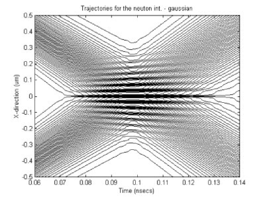
Figure 2: Trajectories in the region of $I$.

To calculate the trajectories, we must first write wave function (8) in the form $\Psi=R\mbox{exp}[iS]$ and then find the expression for $S$, which will be of the form

$$S(\mathbf{r}_{a},t)=G(R_{1},R_{2},S_{1},S_{2},t).$$ (24)

We can then use this expression in the subsidiary condition, $\mathbf{p}=\nabla S$ to calculate the trajectories. These are straightforward to evaluate numerically. The trajectories in the region $I$ and its immediate surroundings are shown in figure 2.

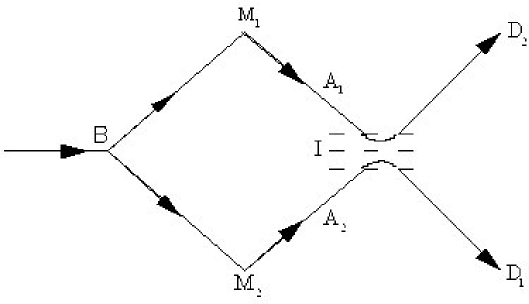
Figure 3: Sketch of particle trajectories.

The complete trajectories from the beam splitter to the detectors have then been sketched in figure 3 for convenience. These figures show that the atoms that are ultimately detected at D₁ must have travelled along a path BM₂A₂D₁, while the atom that is recorded at D₂, must travel along a path BM₁A₁D₂. We immediately see here that the trajectories appear to be reflected about the $z=0$ plane. It is this result that seems to be totally against ‘common sense’ and therefore there must be something wrong with the Bohm approach. However it should be noted that these results are entirely consistent with the quantum probability currents that we discussed in section 3 where we showed that there was no net current crossing the $z=0$ plane.

How is it possible for trajectories to be reflected in the way shown in a region free of any classical potentials and therefore for no apparent reason?

Actually we do already have a similar type of behaviour in the two-slit interference experiment [30]. After the particles have passed through the slits, they no longer follow straight-line trajectories, but show a series of ‘kinks’. None of these trajectories cross the horizontal plane of symmetry. All the particles that pass through the top slit end up on the top part of the plane of the interference pattern. The kinks in the trajectories are just sufficient to create the bunching in exactly the right way to produce the required fringes. The reason for these kinks was immediately seen from the calculation of the quantum potential. This potential changes rapidly in the region of these kinks and is thus seen to be directly responsible for the resulting ‘interference’.

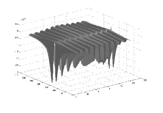
Figure 4: Quantum potential in region $I$.

We can show that a similar quantum potential is responsible for the behaviour of the trajectories crossing region $I$ in the interferometer we are considering here. We can calculate this quantum potential $Q$, using the wave function $\psi(\mathbf{r}_{a})$ to obtain an expression for the amplitude $R$

$$R(\mathbf{r}_{a},t)=F(R_{1},R_{2},S_{1},S_{2},t)$$ (25)

The result of the calculation for $Q$ is shown in figure 4.

This behaviour is exactly what we would expect in a region where the wave functions overlap. A close examination of the details of the potential shows that it exactly accounts for the shape of the trajectories shown in figure 2. In this way we have an explanation of why the Bohm trajectories are reflected in the $z=0$ plane and we have a causal explanation of why the trajectories behave as they do. It is this feature that leads to the conclusion that ‘Bohm trajectories do not cross’.

5.2 Trajectories with the cavity in place

As we have seen the serious challenge made by ESSW2 arises when the micromaser cavity is added to one of the arms of the interferometer as shown in figure 1. To discuss the consequences of adding this cavity for the Bohm trajectories, we can simplify the problem considerably by following Dewdney et al [10] and replacing the cavity by a particle in a one-dimensional ‘box’ described by two wave functions, $\Phi_{0}(\mathbf{r}_{b})$ for the unexcited state and $\Phi_{E}(\mathbf{r}_{b})$ for the excited state. Here $\mathbf{r}_{b}$ is the position co-ordinate of the particle in the box. We will continue to assume that the wave functions of the atom, $\psi_{1}(\mathbf{r}_{a},t)$ and $\psi_{2}(\mathbf{r}_{a},t)$, are Gaussians of small width.

The wave function for the system at time $t_{1}$ after the atom has sufficient time to interact with the ‘cavity’, but not yet had time for their the Gaussian wave packets to overlap (i.e., they have not yet reached the region $I$) will be either

$$\Psi(\mathbf{r}_{a},\mathbf{r}_{b},t_{1})=\psi_{1}(\mathbf{r}_{a},t_{1})\Phi_{0}(\mathbf{r}_{b})$$ (26)

or

$$\Psi(\mathbf{r}_{a},\mathbf{r}_{b},t_{1})=\psi_{2}(\mathbf{r}_{a},t_{1})\Phi_{E}(\mathbf{r}_{b})$$ (27)

By using the method described in section 3.1, the set of trajectories centred on BM₁A₁ can be calculated using equation (26), while those centred on BM₂A₂ can be calculated from equation (27).

We can check that these give the expected outcome by moving the detectors D₁ and D₂ to the positions A₁ and A₂ (See figure 5 below). We will then be able to confirm that the atom that goes through the ‘cavity’ will be recorded D₂, while the atom that does not go through the ‘cavity’ will be recorded at D₁. In the first case, the energy of this atom should, of course, be less since it has exchanged energy with the ‘cavity’, and this can be checked by putting an energy-measuring device, D₄, at A₂. All of this is exactly as we would expect and no strange or unacceptable behaviour results at this stage.

As we have seen the problem arises once we allow the Gaussian wave packets to overlap again in the region of interference $I$. Since we have assumed that there is no coherence loss when the atom has passed through the ‘cavity’, the wave function must now be written in the form

$$\Psi(\mathbf{r}_{a},\mathbf{r}_{b},t_{1})=\psi_{1}(\mathbf{r}_{a},t_{1})\Phi_{0}(\mathbf{r}_{b})+\psi_{2}(\mathbf{r}_{a},t_{1})\Phi_{E}(\mathbf{r}_{b})$$ (28)

Let us now examine what happens in the region of interference $I$ in this case. The wave functions $\Phi_{0}(\mathbf{r}_{b})$ and $\Phi_{E}(\mathbf{r}_{b})$ are both real so that equation (28) can be written in the form

$$\Psi_{f}(\mathbf{r}_{a},\mathbf{r}_{b},t)=R_{1}(\mathbf{r}_{a},\mathbf{r}_{b},t)exp[iS_{1}(\mathbf{r}_{a},t)]+R_{2}(\mathbf{r}_{a},\mathbf{r}_{b},t)exp[iS_{2}(\mathbf{r}_{a},t)]$$ (29)

In order to calculate the trajectories, we must again write this wave function in the form

$$\Psi_{f}(\mathbf{r}_{a},\mathbf{r}_{b},t)=R(\mathbf{r}_{a},\mathbf{r}_{b},t)exp[iS(\mathbf{r}_{a},\mathbf{r}_{b},t)]$$ (30)

We immediately see an important difference between this case and the case described by equation (23). Here $R$ and $S$ are functions of both $\mathbf{r}_{a}$ and $\mathbf{r}_{b}$, rather than $\mathbf{r}_{a}$ alone and therefore we have a pair of coupled one-parameter solutions of the real part of the Schrödinger equation. These are given by

$$\mathbf{p}_{a}=\nabla_{{\mathbf{r}_{a}}}S(\mathbf{r}_{a},\mathbf{r}_{b},t)\hskip 28.45274pt\mbox{and}\hskip 28.45274pt\mathbf{p}_{b}=\nabla_{{\mathbf{r}_{b}}}S(\mathbf{r}_{a},\mathbf{r}_{b,t})$$ (31)

This means that as the atom moves along its trajectory in the region of interference, $I$, the particle in the box also moves, showing that this particle is still coupled to the atom even though they are separated in space. This would then also account for why the probability current for the ‘particle in the box’ (the cavity) discussed in section 3 is different from zero as the atom passes through the region $I$.

From the classical point of view this behaviour would be absurd. However when we examine this more closely, we find that it is the quantum potential that mediates this coupling, and recall this coupling is a necessary consequence of the Schrödinger equation and is not an arbitrary feature imposed from the outside to satisfy some metaphysical pre-requisite.

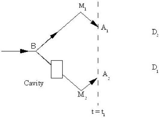
Figure 5: Trajectories at time $t=t_{1}$.

What makes this quantum potential seem particularly unpalatable is its gross non-locality or non-separability. Here we have the surprising feature that the atom and the ‘cavity’ are still coupled long after the atom should have passed (or not passed) through the ‘cavity’. The process is not complete once the wave packet has passed through the cavity. This is a very clear example of why Wheeler argues that the process is “brought to a close by an irreversible act of amplification”.

However this behaviour should not be so surprising, it is exactly the situation found in the EPR paradox [31] and, indeed in quantum teleportation [32]. It is the quantum potential that provides an explanation of these effects and one can see that this coupling is essential to conserve energy. (For further details of this point see Hiley [17]).

Let us now go on to examine the trajectories of the atom in detail. Four sets of trajectories for particular sets of initial conditions $\{\mathbf{r}_{a_{0}}\}$, and for four different values of $\mathbf{r}_{b_{0}}$ are shown in figure 6. These trajectories exhibit ‘wobbles’ that are a typical signature for interference-type behaviour and these are a necessary consequence of the coherence between the two wave packets.

Does this mean that the Bohm approach predicts interference in the region $I$? If this were the case, the Bohm interpretation would clearly disagree with the standard interpretation, which predicts that there are no visible interference effects in the region $I$ and indeed no fringes are visible in this region.

As we have already shown in section 2, the wave function is given by equation (1) which gives no interference fringes because $\Phi_{0}(\mathbf{r}_{b})$ and $\Phi_{E}(\mathbf{r}_{b})$ are orthogonal. In other words integrating over all $\mathbf{r}_{b}$, destroys the interference terms. This integration over $\mathbf{r}_{b}$ provides the clue as to why the Bohm approach does not predict any interference effects either. Although each particular set of trajectories shown in figure 6 do show interference-type ‘wobbles’, they do so only for the curves calculated for a given $\mathbf{r}_{b_{0}}$.

When we average over the ensemble of trajectories over different initial $\mathbf{r}_{b_{0}}$, no interference effects appear in the region $I$. This is because the set of positions of this ensemble at some time $t=t_{2}$ when the atoms would be in the region, $I$, show a uniform distribution, rather than a fringe pattern. Thus the total of all Bohm trajectories do not bunch to form an interference pattern so there is no disagreement with quantum mechanics on this point.

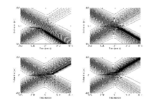
Figure 6: Trajectories for four different $\mathbf{r}_{b0}$.

Now we come to the crucial point from which the objections have been raised. The calculations for different $\mathbf{r}_{b}$ show that a significant number, although by no means all, of the trajectories will be similar to those illustrated in figure 4. That is they will be ‘reflected’ in the region of overlap and it is the presence of this type of trajectory that led ESSW2 to the conclusion that the trajectories must be rejected because of their bizarre behaviour. Their argument runs as follows.

Suppose an atom follows the trajectory BCM₂A₂D₁. On passing through C it gives up energy to the ‘cavity’, as we have already seen when we discussed what happened when we measured the energy of an atom at A₂. But according to the trajectory picture any atom on that path would have ended up in the detector D₁.

If we were to measure the energy of this atom just prior to entering D₁, we would find that it had NOT lost any energy. Indeed its wave function is $\psi_{1}(\mathbf{r}_{a})$ which indicates it must have the same energy as when it entered the beam-splitter B. There is no loss of energy because if we also measure the energy of the ‘cavity’ at any time after the atom had left region $I$, we would have found that it had NOT gained any energy! Yet any energy measurement prior to the atom reaching the region $I$ would show that the atom had lost energy to the ‘cavity’ and the ‘cavity’ had gained energy. It is this feature that is very surprising and which is used to suggest that the Bohm approach is flawed.

Of course a similar argument can also be applied to an atom that ends up at D₂ after following the trajectory BM₁A₁. In this case a measurement of its energy just before it arrived at D₂ would show that it had lost energy to the ‘cavity’ even though it had not been anywhere near the ‘cavity’. How could this possibly happen?

Clearly if an atom that goes through a ‘cavity’ without exciting it, or conversely, if an atom that does not go through the ‘cavity’ succeeds in exciting it without any apparent connection between atom and ‘cavity’, must be regarded as behaving ‘unreasonably’. In this case we would be forced to conclude that the trajectories do not have any physical meaning. However the crucial phrase is “without any apparent connection between atom and cavity”.

As we have already explained there is a ‘connection’ between the atom and the ‘cavity’. The connection appears in the real part of the Schrödinger equation itself where it takes the form of the quantum potential. ESSW2 have completely ignored this aspect of the Bohm ontology. For as Bohm and Hiley [36] point out, one of the key features of the ontology is that “This particle is never separate from a new type of field that fundamentally affects it. This field is given by $R$ and $S$ or alternatively by $\psi=R\mbox{exp}[iS]$. $\psi$ then satisfies Schrödinger’s equation (rather than, for example, Maxwell’s equation), so that it too changes continuously and is causally determined.”

Thus the quantum potential is an essential part of the description. Without taking the causally determined field into account and only giving relevance to the trajectories derived from the guidance condition, it is not surprising that the resulting behaviour has been regarded as ‘unacceptable’.

5.3 Detailed account of the Bohm trajectories

Consider the atom as it moves along the path BCM₂A₂. As it passes through the ‘cavity’, an interaction Hamiltonian couples the wave function representing the atom to wave function of the ‘cavity’ causing it to change, as well as inducing a corresponding change in the wave packet of the atom. After the interaction has finished, the wave function of the ‘cavity’ (in this case the particle in the box) is real. The Bohmian approach then shows that the particle in the box is stationary and in consequence any excitation energy of the ‘cavity’ is stored entirely as quantum potential energy.

As the atom passes through the interference region $I$, a new quantum potential energy is generated. It must be emphasised that since this energy arises from equation (25) using equation (1), it must of necessity include the quantum potential energy stored in the ‘cavity’. It is this coupling that gives rise to any exchange of energy between the ‘cavity’ and the atom so that when the atom emerges from the region $I$, it has regained its original energy and the ‘cavity’ is no longer excited. In other words the process has been truly ‘erased’.

If the particle follows the other route, the ‘cavity’ is not excited until the particle reaches the region of interference. Here the wave packet carrying information about the ‘cavity’ comes into effect and energy, in the form of quantum potential energy, is again redistributed so that the cavity becomes excited and the atom loses energy if it is travelling along one of the ‘reflected’ trajectories.

Notice that no external energy is involved in this process. It is merely a re-distribution of internal energy of the two systems linked by the wave function (1). This is merely another way of demonstrating what Bohr [16] called the ‘wholeness of the phenomenon’. The two spatially separated systems still form a totality until an irreversible change takes place. After this change the two systems become independent uncoupled systems.

If we look at this behaviour from the standpoint of classical physics of course the explanation seems bizarre. The classical particle is the centre of the activity and all energy is either kinetic energy or the potential energy arising from an interaction with some external system. In this case all energy exchanges must occur only through a local interaction between the particle and any externally applied force.

Quantum phenomena have an inner structure that cannot be sharply divided into separate sub-systems interacting only through classical forces described mathematically by a Hamiltonian. However if we do separate a system into sub-systems, as we do in the Bohm approach, then it is necessary to have some feature that reflects this relationship of ‘indivisibility’ between these sub-systems and this feature is provided by the quantum potential [37]. Thus the quantum potential reflects the essential ‘non-separability’ or ‘wholeness’ of quantum processes that Bohr recognised to lie at the heart of quantum processes. This is the reason why the quantum potential plays an essential role in the Bohm approach.

In the above analysis we are forced to attribute new properties to the particle and to the quantum potential that are totally different from those associated with classical particles and classical potentials. If one refuses to recognise the need for these novel properties, which we regard to be essential to obtain a consistent interpretation of the formalism, then it is very easy to ridicule the approach. All one has to do is to contrast these properties with those of classical physics and to conclude there are ‘unacceptable’ and ‘surreal’.

5.4 Replacement of Cavity by an Energy Measuring Device D₃

In order to complete the technical side of the discussion, let us replace the ‘cavity’ with a “position detector” D₃ as shown in figure 7 below. We will assume this detector has 100$\%$ efficiency and let us further assume, for the present, that the atom emerging from D₃ can be described by a wave function $\psi_{2}(\mathbf{r}_{a})$ , which is still coherent with $\psi_{1}(\mathbf{r}_{a})$. The wave function in this case would be

$$\Psi(\mathbf{r}_{a},\mathbf{r}_{c},\mathbf{r}_{d},t_{3})=\psi_{1}(\mathbf{r}_{a},t_{3})\Lambda_{unfired}(\mathbf{r}_{c},t_{3})\Omega_{unfired}(\mathbf{r}_{d},t_{3})$$

$$+\psi_{2}(\mathbf{r}_{a},t_{3})\Lambda_{fired}(\mathbf{r}_{c},t_{3})\Omega_{fired}(\mathbf{r}_{d},t_{3})$$ (32)

where $\Lambda_{i}(\mathbf{r}_{c},t_{3})$ are the wave functions of the detector D₃ and $\Omega_{i}(\mathbf{r}_{d},t_{3})$ are the wave functions of detector D₂.

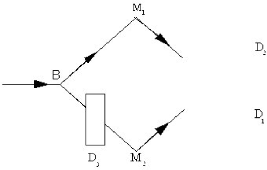
Figure 7: Interferometer with position detector D₃ in place.

Here one could argue that because of the rule “Bohm trajectories do not cross”, we will still obtain the odd behaviour of the ‘trajectories’ of the type shown in figure 2 as they cross the region $I$. For example, we know from the wave function (1) that D₂ will always fire after D₃ has fired. The ‘no-crossing’ rule for Bohmian trajectories would suggest that the atom should travel along the path BM₁D₂. This would mean that D₃ had fired even though the particle had not gone through D₃. This looks as if we will have a situation similar to the case of the ‘cavity’.

However this is not correct. On detection in D₃ an irreversible record is left in the device. If we were forced to use the explanation that in this case we still need an exchange of nonlocal energy, then we would see this ‘irreversible’ mark disappear from the recording of the detector D₃ as the atom passes through the region $I$. This would, indeed, be totally unacceptable and would stretch the plausibility of the assumption that the one-parameter solutions of equation (19) are particle trajectories. Fortunately this situation does not occur in the Bohm interpretation.

To show this let us consider the wave function after the particle has sufficient time, $t=t_{2}$, to pass M₁ or M₂, but before it reaches the detector D₂

$$\Psi(\mathbf{r}_{a},\mathbf{r}_{c},\mathbf{r}_{d},t_{3})=[\psi_{1}(\mathbf{r}_{a},t_{3})\Lambda_{unfired}(\mathbf{r}_{c},t_{3})$$

$$+\psi_{2}(\mathbf{r}_{a},t_{3})\Lambda_{fired}(\mathbf{r}_{c},t_{3})]\Omega_{unfired}(\mathbf{r}_{d},t_{3})$$ (33)

We can again ask what happens in region $I$. Let us begin by calculating the quantum potential in the region $I$. Will it still contain interference terms or not?

To answer this question we must first write

$$\Psi_{final}=R_{f}(\mathbf{r}_{a},\mathbf{r}_{c},t_{2})exp[iS_{f}(\mathbf{r}_{a},\mathbf{r}_{c},t_{2})]$$ (34)

with

$$R_{f}(\mathbf{r}_{a},\mathbf{r}_{c},t_{2})=K[R_{uf1}(\mathbf{r}_{a},\mathbf{r}_{c},t_{2}),R_{f2}(\mathbf{r}_{a},\mathbf{r}_{c},t_{2}),S_{uf1}(\mathbf{r}_{a},\mathbf{r}_{c},t_{2})S_{f2}(\mathbf{r}_{a},\mathbf{r}_{c},t_{2})]$$ (35)

and

$$S_{f}(\mathbf{r}_{a},\mathbf{r}_{c},t_{2})=L[R_{uf1}(\mathbf{r}_{a},\mathbf{r}_{c},t_{2}),R_{f2}(\mathbf{r}_{a},\mathbf{r}_{c},t_{2}),S_{uf1}(\mathbf{r}_{a},\mathbf{r}_{c},t_{2})S_{f2}(\mathbf{r}_{a},\mathbf{r}_{c},t_{2})]$$ (36)

From equation (35), we can evaluate the quantum potential acting on the particle using

$$Q_{f}(\mathbf{r}_{a},\mathbf{r}_{c},t)=-\frac{1}{2m}\frac{\nabla_{\mathbf{r}_{a}}^{2}R_{f}(\mathbf{r}_{a},\mathbf{r}_{c},t)}{R_{f}(\mathbf{r}_{a},\mathbf{r}_{c},t)}$$ (37)

This must be evaluated at the final positions of the set of values of $\{\mathbf{r}_{c}\}$.

If D₃ is to be a measuring device, then the position of the two sets of variables for the fired and unfired states must be sufficiently different so that the two final states of D₃ can be clearly distinguished. This is equivalent to requiring the wave packets describing the two possible D₃ states not to be overlapping in the variables $\{\mathbf{r}_{c}\}$. Because of this requirement, if D₃ does not fire, the contribution to the quantum potential $Q_{f}$ will only come from $R_{uf1}$ and $S_{uf1}$. The other two terms, $R_{f2}$ and $S_{f2}$ will not contribute to $Q_{f}$ because they are zero when the set $\{\mathbf{r}_{c,unfired}\}$ is substituted in to equation (32).

On the other hand if D₃ does fire, then the contributions to $Q_{f}$ will only come from $R_{f2}$ and $S_{f2}$, because the other two terms will be zero when evaluated at the positions set $\{\mathbf{r}_{c,fired}\}$.

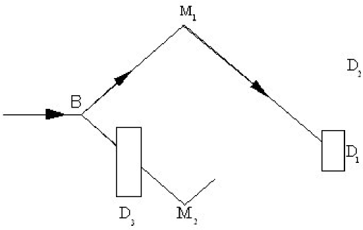
Figure 8: Detector D₃ does not fire.

Thus $Q_{f}$ will never contain contributions from the path that the particle did not take. In consequence there will be no interference terms so the two possible paths will be

1. BM₁D₁ if D₃ does not fire so that D₁ does fire. (See figure 8)

2. BD₃M₂D₂ if D₃ does fire. In this case D₂ will fire. (See figure 9)

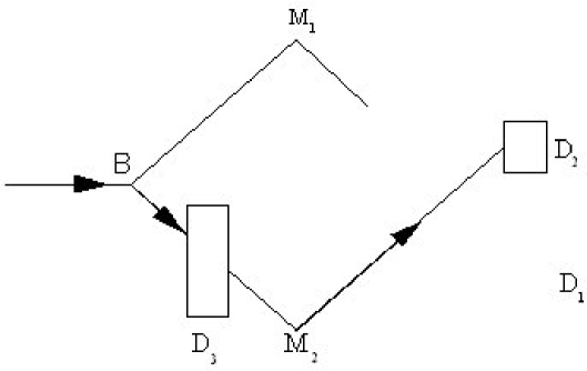
Figure 9: Detector D₃ fires.

The particle trajectories are therefore straight lines from M₁ to D₁ if D₃ does not fire, or straight lines from M₂ to D₂ if D₃ does fire. Thus both sets of trajectories pass straight through the region $I$ without showing any coherence. This is exactly the situation described by the density operator

$$\rho=|\psi_{1}\rangle|\Lambda_{unfired}\rangle\langle\psi_{1}|\langle\Lambda_{unfired}|+|\psi_{2}\rangle|\Lambda_{fired}\rangle\langle\psi_{2}|\langle\Lambda_{fired}|$$ (38)

The consequences of this density operator are the same as those described in section 2.

In this case the rule that “Bohm trajectories do not cross” is not violated because the relevant space in which the non-crossing rule works is configuration space. The introduction of the detector D₃ increases the number of dimensions of the configuration space to include the set $\{\mathbf{r}_{c}\}$ of relevant detector particles. What this means is that each trajectory is parameterised by $\mathbf{r}_{a}$ and $\{\mathbf{r}_{c}\}$. Since the set $\{\mathbf{r}_{c,fired}\}$ and the set $\{\mathbf{r}_{c,unfired}\}$ are distinct, the set of trajectories corresponding to when D₃ fires is distinct from the set when D₃ does not fire and therefore the trajectories corresponding to each situation do not cross in the higher dimensional configuration space. The trajectories only appear to cross when they are projected into the two-dimensional ($\mathbf{r}_{a}$ ) configuration space. Thus there is no violation of the “no crossing” rule.

This completes the detailed description of the Bohm trajectories in the various possible structures that arise in the type of interferometer arrangements discussed by ESSW2, ESSW3 and Scully [9].

5.5 The criticisms of Aharonov and Vaidman

Finally we want to consider the criticisms of Aharonov and Vaidman [14]. Although they are mainly to do with a model that is fundamentally different from that considered in this paper, they have drawn attention to a problem that is perceived to present a problem for the Bohm approach we are using here.

The problem involves replacing the cavity with a bubble chamber and replacing the atoms with particles that can ionise the liquid molecules in the bubble chamber. Aharonov and Vaidman argue that

The bubbles created due to the passage of the particle are developed slowly enough such that during the time of motion of the particle the density of the spatial wave function of each bubble does not change significantly.

In this case they argue that we will see the trace of the bubbles behaving as if the particle moves in one arm, whereas it actually travels down the other arm.

We will now show that this does not happen. To do this we must be much more careful in analysing the process that is responsible for the bubbles forming in the first place. The starting point for the development of a bubble is an ionised atom or molecule that provides the nucleus for a bubble to form in the first place. Let us simplify the discussion by discussing the interaction of the particle with one atom of the bubble chamber liquid. Let the wave function of the un-ionised atom be $\Psi_{UA}(\mathbf{r}_{A},\mathbf{r}_{e})$ where $\mathbf{r}_{A}$ is the centre of mass co-ordinate of the atom and $\mathbf{r}_{e}$ is the position of the electron that will be ejected from the atom. After the ionising interaction has taken place, the wave function of the ionised atom will be $\Psi_{IA}(\mathbf{r}_{A})$ and the wave function of the ejected electron will be $\phi(\mathbf{r}_{e})$. The total wave function at time $t=t_{1}$ will be

$$\Psi(\mathbf{r}_{a},\mathbf{r}_{A},\mathbf{r}_{e},t_{1})=\psi_{1}(\mathbf{r}_{a})\Psi_{UA}(\mathbf{r}_{A},\mathbf{r}_{e})+\psi_{2}(\mathbf{r}_{a})\Psi_{IA}(\mathbf{r}_{A})\phi(\mathbf{r}_{e})$$ (39)

Before the bubble can begin to form on the ionised atom, the electron must be removed a sufficient distance so that the probability of finding the electron at the atom is zero. This means that the wave function of the ionised atom does not overlap with the wave function of the electron. We can now write this wave function in the form

$$\Psi_{final}=R_{f}(\mathbf{r}_{a},\mathbf{r}_{A},\mathbf{r}_{e},t_{1})\mbox{exp}[iS_{f}(\mathbf{r}_{a},\mathbf{r}_{A},\mathbf{r}_{e},t_{1})]$$ (40)

We can then evaluate the quantum potential and find that it contains no interference terms. Once again the reason for this is that the expression must be evaluated for the positions of all the particles.

If the particle does not ionise the molecule, ie, it travels on the path BM₁A₁ then the contribution of the second term will be zero because the electron will be in the position where $\phi(\mathbf{r}_{e})$ is zero. On the other hand if the particle does ionise the atom, the first term will give no contribution to the quantum potential because $\Psi_{UA}(\mathbf{r}_{A},\mathbf{r}_{e})$ is zero for the ionised position of the electron. This means that when ionisation is involved, the wave function (39) effectively behaves like the density operator as far as the Bohm approach is concerned. In other words the two paths do not produce any interference effects, so the particle either follows the path BM₁A₁D₁ or BM₂A₂D₂. Thus the particle that ionises the atoms of the liquid actually pass through the points that eventually develop into the bubble track. It does not matter how slowly the bubbles develop, it is the ionisation process that destroys any interference effects in the cross-over region $I$. Thus the Bohm approach when evaluated correctly does not give the results claimed for it by Aharonov and Vaidman [14].

6 Conclusions

In this paper we have shown that the claim that we can meaningfully talk about particle trajectories in an interferometer such as the one shown in figure 1 within quantum mechanics made by ESSW2 [8] and by Scully [9] does not follow from the standard (Copenhagen) interpretation. An additional assumption must be made, namely, that the cavity and the atom can only exchange energy when the atom actually passes through the cavity. Here the position of the particle becomes an additional parameter, which supplements the wave function and therefore is not part of the orthodox interpretation. Furthermore we have shown that this way of introducing the position coordinate leads to a contradiction as we are forced to conclude that although the atom follows one path, it behaves as if it went down both paths.

In standard quantum mechanics, inferences about the ‘path’ of a particle can only be made in terms of a series of measurements. As Heisenberg [21] states “By path we understand a series of points in space which the electron takes as ‘positions’ one after another.” He adds: “When one wants to be clear about what is to be understood by the words ‘position of the object’, then one must specify definite experiments with whose help one plans to measure the ‘position of the electron’; otherwise this word has no meaning”.

The claim by Scully [9] is that the cavity constitutes a potential position-measuring device cannot be sustained. A measuring device giving rise to an observation requires, according to Bohr [13], some form of amplification that involves an irreversible process. An exchange of energy with the cavity per se does not involve any amplification or irreversible process and therefore the cavity does not constitute a position-measuring device in the sense assumed in the orthodox interpretation of quantum mechanics. This means that the addition of the cavity to one arm of an interferometer cannot be used as a Welcher Weg (WW)device from within the Copenhagen interpretation.

Of course, the subsequent measurement of the energy of the cavity does involve amplification and irreversibility. But as we have seen in section 2, the cavity cannot be taken to be a position-measuring device once the atom has passed through the region of interference I without an additional assumption, which we have shown leads to the contradiction discussed above.

Even when discussing energy exchanges, the orthodox interpretation insists on using only the wave function, without reference to any additional parameters such as the particle s actual position. That is the interaction Hamiltonian only introduces changes in the wave functions of the particle and the cavity independently of the actual position of the particle. Recall the quotation of Bohr [20] given in section 2.1 where he points out that the impossibility of sub-dividing quantum phenomena leads to an ambiguity in attributing physical properties to atomic objects and this ambiguity demands a description being given only in terms of wave functions. Thus not only is it unnecessary to insist that the particle must have been through the cavity, it actually has no meaning to make such a claim.

Indeed as Bohr points out, we cannot sub-divide a quantum process and analyse it in the way we do in classical physics. All we can rely on is the well-defined quantum algorithm from which we are able to calculate the probabilities of a given outcome defined by the whole experimental arrangement [13]. This process does not attach any notion of reality to the wave function; it is regarded simply as part of the mathematical algorithm, or if you will a ‘tool’, giving it no ontological status at all. It is merely a symbol in a mathematical formula and as long as we adopt this position we cannot talk about which way particles go when interference is involved. If we want to give direct significance to the particle and remain in total agreement with the quantum formalism then we must use the Bohm approach.

In fact in section 5 we have provided a complete account of the Bohm interpretation as applied to the interferometer introduced by ESSW2 and Scully. We have shown that the observational consequences of the Bohm approach are exactly the same as those obtained from the orthodox interpretation when the cavity is in place. To prevent any further misunderstanding of the consequences of the Bohm approach we will summarise the results in the various situations involving the interferometer shown in figure 1.

If energy measurements are made at a time $t=t_{1}$ (see figure 6) by inserting the device at A₁ or A₂ then

1. The atom arriving at A₁ will be excited and no energy will be detected in the cavity.

2. The atom arriving at A₂ will have lost its energy and the cavity will be excited.

If the energy measurements are made at time $t=t_{3}$ when the wave packets $\psi_{1}(\mathbf{r}_{a})$ and $\psi_{2}(\mathbf{r}_{a})$ have again separated after passing through the region $I$, then

3. The atoms arriving at D₁ (see figure 1) will have retained their energy and the cavity will be unexcited.

4. The atoms arriving at D₂ (see figure 1) will have lost their energy and the cavity will be excited.

These predictions are exactly the same as those obtained from standard quantum mechanics. There are no observable differences between standard quantum mechanics and the Bohm approach nor can there be simply because the Bohm approach uses the same wave functions and the same formalism as is used in the usual approach and therefore both approaches must end up with exactly the same probabilities. Because we are using in addition the one-parameter solutions of the real part of the Schrödinger equation given in (19) we get a further insight into quantum phenomena.

The Bohm way of looking at the solutions avoids some of the difficulties presented by the standard approach. It has no ambiguity in the role played by the ‘quantum particle’. It has no measurement problem and definitely no schizophrenic cats. It offers an explanation of the behaviour of the probability currents discussed in section 3 and it also clearly shows why the cavity cannot be used as a WW device. It also draws attention to the non-separability and non-locality aspects of systems described by entangled wave functions, a feature that Bohr was content to describe as the inherent ‘wholeness of the phenomenon’.

In spite of these positive aspects a word of caution should is necessary. There is no way to confirm that the quantum process is actually a particle travelling along a path which is separate from the $R$ and $S$ fields. These fields are not classical fields that are to be included in a Hamiltonian and are not independent of the particle itself. They have a very different quality from the fields that arise in classical physics and this suggests that there is a radically novel ontological process involved that the Bohm approach captures in some coarse-grained approximation.

Bohm and Hiley[3][2] have suggested that these new fields can be understood in terms of the new concept of active information, a concept that has been discussed elsewhere (Maroney and Hiley [32], Hiley [17] and Hiley and Pylkkänen [38]). In spite of these limited successes, the nature of this deeper process is still very illusive and arises essentially from the non-commutative structure of the quantum algebra.

In quantum mechanics these non-commutative algebras have a profound implication for the nature of spacetime, as is very clear from some of the attempts to understand non-commutative geometry (Connes [39]). Some of these ideas have been applied to the EPR paradox offering a possible understanding of non-locality through a deeper understanding of the properties of spacetime (Grib and Zapatrin [40], Hiley [41], Hiley and Fernandes [42], Heller and Sasin [43]). These papers move the discussion about the nature of quantum non-separability and quantum non-locality on to a new level away from the somewhat sterile discussions on the interpretation of the non-relativistic quantum formalism.

7 References

References

- [1] D. Bohm, 1952, A Suggested Interpretation of the Quantum Theory in Terms of Hidden Variables , Phys. Rev., 85, 166-179; 85, 180-193.
- [2] D. Bohm and B. J. Hiley, 1987, An Ontological Basis for the Quantum Theory: I-Non-relativistic Particle Systems, Phys. Reports 144, 323-348.
- [3] D. Bohm and B. J. Hiley, 1993, The Undivided Universe: an Ontological Interpretation of Quantum Theory, Routledge, London.
- [4] P. Holland, 1993, The Quantum Theory of Motion, Cambridge University Press, Cambridge.
- [5] D. Dürr, S. Goldstein and N. Zanghi, 1992, Quantum Equilibrium and the Origin of Absolute Uncertainty, J. Stat. Phys., 67, 843-907.
- [6] W. Pauli, 1953, Remarques sur le problèm des paramètres cach s dans la m chanique quantque et sur la th orie de l onde pilote, in Louis de Broglie, Physicien et Penseur, ed A. George, 3-42, Èditions Albin Michel, Paris.
- [7] H. D. Zeh, 1998, Why Bohm’s Quantum Theory? quant-phy/9812059.
- [8] B-G. Englert, M. O. Scully, G. Sussman and H. Walther, (ESSW2), 1992, Surrealistic Bohm Trajectories, Z. Naturforsch. 47a, 1175-1186.
- [9] M. O. Scully, 1998, Do Bohm trajectories always provide a trustworthy physical picture of particle motion? Phys. Scripta, T76, 41-46.
- [10] C. Dewdney, L. Hardy and E. J. Squires, 1993, How late measurements of quantum trajectories can fool a detector, Phys. Lett. 184A, 6-11.
- [11] D. Dürr, W. Fusseder, S. Goldstein and N. Zanghi, 1993, Comment on “Surrealistic Bohm Trajectories”, Z. Naturforsch. 48a, 1261-1262.
- [12] B-G. Englert, M. O. Scully, G. Sussman and H. Walther, (ESSW3), 1993, Reply to Comment on “Surrealistic Bohm Trajectories, Z. Naturforsch. 48a, 1263-1264.
- [13] N. Bohr, 1961, Atomic Physics and Human Knowledge, Science Editions, New York.
- [14] Y. Aharonov and L. Vaidman, 1996, in Bohmian Mechanics and Quantum Theory: an Appraisal, ed J. T. Cushing, A. Fine and S. Goldstein, Boston Studies in the Philosophy of Science, 184, 141-154, Kluwer, Dordrecht.
- [15] R. B. Griffiths, 1999, Bohmian mechanics and consistent histories, Phys. Lett., A261, 227-234.
- [16] N. Bohr, 1961, Atomic Physics and Human Knowledge, p. 39, Science Editions, New York.
- [17] B. J. Hiley, 1999, Active Information and Teleportation. In Epistemological and Experimental Perspectives on Quantum Physics, ed. D. Greenberger et al., 113-126, Kluwer, Netherlands.
- [18] A. Einstein, B. Podolsky, and N. Rosen, 1935, Can Quantum-Mechanical Description of Physical Reality be Considered Complete? Phys. Rev., 47, 777-80.
- [19] L. D. Landau and E. M. Lifshitz, 1977, Quantum Mechanics, p. 2 Pergamon Press, Oxford.
- [20] N. Bohr, 1961, Atomic Physics and Human Knowledge, p. 51, Science Editions, New York.
- [21] W. Heisenberg, 1927, Über den anschaulichen Inhalt der quantumtheoretischen Kinematik und Mechanik, Zeit. f r Phys. 43, 172-98. English translation in J. A. Wheeler and W. Zurek, 1981, Quantum Theory and Measurement, p. 63-5.
- [22] N. Bohr 1951, in Albert Einstein: Philosopher-Physicist ed, P. A. Shilpp, p. 222, Tudor, New York.
- [23] W. Heisenberg, 1958, Physics and Philosophy, Harper-Row, New York, Or The representations of the nature of contemporary physics, Daedalus, 87, 95-108.
- [24] M. O. Scully, B.-G. Englert and H. Walther,1991, Quantum Optical Tests of Complementarity, Nature, 351,111-116.
- [25] N. Bohr, 1961, Atomic Physics and Human Knowledge, p. 64, Science Editions, New York.
- [26] J. A. Wheeler, 1996, At Home in the Universe, p. 344, AIP, New York.
- [27] N. Bohr, 1935,Can quantum-mechanical description of physical reality be considered complete?, Phys. Rev., 48, 696-702.
- [28] J. S. Bell, 1964, On the Einstein-Podolsky-Rosen paradox, Physics, 1, 195-200.
- [29] J. S. Bell, 1966, On the problem of hidden variables in quantum theory, Rev. Mod. Phys. 38, 447-452.
- [30] C. Dewdney, C. Philippidis and B. J. Hiley, 1979, Quantum Interference and the Quantum Potential, Il Nuovo Cimento 52B, 15-28.
- [31] D. Bohm and B. J. Hiley, 1975, On the Intuitive Understanding of Nonlocality as Implied by Qauntum Theory, Found. Phys., 5, 93-109.
- [32] O. Maroney and B. J. Hiley, 1999, Quantum State Teleportation understood through the Bohm Interpretation, Found. Phys. 29, 1403-15.
- [33] D. Bohm, B. J. Hiley and P.N. Kaloyerou, 1987, An Ontological Basis for the Quantum Theory: II -A Causal Interpretation of Quantum Fields, Phys. Reports 144, 349-375.
- [34] P. N. Kaloyerou, 1994, The Causal Interpretation of the Electromagnetic Field, Phys. Rep. 244, 287-385.
- [35] M. M. Lam and C. Dewdney, The Bohm Approach to Cavity Quantum Scalar Field Dynamics, I and II, Found. Phys. 24, 3-60, (1994).
- [36] D. Bohm and B. J. Hiley, 1993a, The Undivided Universe: an Ontological Interpretation of Quantum Theory, p. 29, Routledge, London.
- [37] D. Bohm and B. J. Hiley, 1981, Non-locality in Quantum Theory understood in Terms of Einstein’s Non-linear Field Approach, Found. Phys. 11, 529-546.
- [38] B. J. Hiley and P. Pylkkänen, 1997, Active Information and Cognitive Science-A Reply to Kieseppä, in Brain, Mind and Physics, ed. P. Pylkkänen, P. Pylkkö, and A. Hautam ki, 64-85, IOS Press, Amsterdam.
- [39] A. Connes, 1994, Noncommutative Geometry, Academic Press, San Diego.
- [40] A. A. Grib and R. R Zapatrin, 1992, Topology Lattice as Quantum Logic, Int. J. Theo. Phys. 31, 1093-1101.
- [41] B. J. Hiley, 1991, Vacuum or Holomovement, in The Philosophy of Vacuum, ed., S. Saunders and H. R. Brown, pp. 217-249, Clarendon Press, Oxford.
- [42] B. J. Hiley and M. Fernandes, 1997, Process and Time, in Time, Temporality and Now, ed., H. Atmanspacher and E. Ruhnau, 365-383, Springer-Verlag.
- [43] M. Heller and W. Sasin, 1998, Einstein-Podolsky-Rosen Experiment from Non-commutative Quantum Gravity, Particles, Fields and Gravitation, p. 234, AIP.