Phase-space picture of resonance creation and avoided crossings

Abstract

Complex coordinate scaling (CCS) is used to calculate resonance eigenvalues and eigenstates for a system consisting of an inverted Gaussian potential and a monochromatic driving field. Floquet eigenvalues and Husimi distributions of resonance eigenfunctions are calculated using two different versions of CCS. The number of resonance states in this system increases as the strength of the driving field is increased, indicating that this system might have increased stability against ionization when the field strength is very high. We find that the newly created resonance states are scarred on unstable periodic orbits of the classical motion. The behavior of these periodic orbits as the field strength is increased may explain why there are more resonance states at high field strengths than at low field strengths. Close examination of an avoided crossing between resonance states shows that this type of avoided crossing does not delocalize the resonance states, although it may lead to interesting effects at certain field strengths.

PACS numbers: 32.80.Rm, 05.45.Mt, 03.65.Sq

I Introduction

The study of time-periodic quantum systems has attracted considerable interest in recent years. One of the primary motivating factors for this interest is the development of ultra-high intensity lasers, which can produce electric fields within atoms that rival those produced by the atomic nucleus. Experiments with these ultra-intense lasers have led to the discovery of many interesting new phenomena, such as high harmonic generation [1]. Simple one-dimensional models of the interaction between intense lasers and atoms have been shown to reproduce, at least qualitatively, many of these interesting phenomena [2]. These models are especially interesting because their classical versions display chaotic motion [3]. In addition to providing insight into recent experiments, the study of these models can also provide insight into quantum-classical correspondence.

One of the more interesting phenomena observed in these systems is the stabilization of atoms in intense laser fields. Stabilization is characterized by a decrease in the probability for an electron to ionize as the laser intensity is increased. This effect was first discovered in theoretical studies of the interaction between high-frequency lasers and atoms [4], but recent experiments have verified that stabilization occurs in real atoms [5, 6]. Studies of the underlying classical dynamics of these systems using one- and two-dimensional models have shown that the classical motion can often account for the increased stability of the atom at higher laser intensities [6, 7].

The study of time-periodic quantum models is usually carried out within the context of Floquet theory [8]. Floquet eigenstates are eigenstates of the one-period time evolution operator and are the natural states for describing time-periodic systems. In some cases the Floquet states of the system can be localized on stable structures in the classical phase space [9], and this can lead to stabilization because these Floquet states have very long lifetimes. In this case, stabilization would also be predicted by the classical dynamics. However, there are often significant differences between the classical and quantum dynamics of chaotic systems. One of the most striking examples of this is scarring, where quantum eigenstates have higher probability to be found near the locations of unstable periodic orbits in the classical phase space [10]. The scarring of Floquet states on unstable periodic orbits might make it possible for a quantum system to exhibit stabilization even when the corresponding classical dynamics is unstable. Some earlier studies indicate that stabilization can be associated with states that are scarred on unstable or weakly stable periodic orbits [11].

In this paper we examine a time-periodic system with one space dimension which shows signs of stabilization. In this system the number of localized Floquet states, or resonance states, increases as the intensity of the driving field is increased. In Sec. II we present the model and discuss the classical dynamics as well as prior studies of the quantum dynamics. In Sec. III we describe two different versions of complex coordinate scaling and compare their predictions in this system. In Sec. IV we investigate the relationship between the resonance states and the classical dynamics of the system. We find that the resonance states that are created as the driving field is increased are associated with unstable periodic orbits in the classical dynamics. We give an explanation, based on this association with periodic orbits, for why the number of resonance states increases as the laser field is increased.

In Sec. V we carry out a detailed study of an avoided crossing between two resonance states. Avoided crossings in time-periodic quantum systems lead to significant changes in the structure of the Floquet states [12, 13]. Overlapping avoided crossings can even lead to delocalization of Floquet states [13]. Since stabilization depends upon the Floquet states remaining localized near (stable or unstable) classical structures, avoided crossings may play an important role in destroying stabilization. Finally, in Sec. VI we summarize our findings.

II Driven Inverted Gaussian Model

The model we will study is an inverted Gaussian potential interacting with a monochromatic driving field in the radiation gauge. The Hamiltonian of the system in atomic units (which are used throughout the paper) is

$$H=\frac{1}{2}\left(p-\frac{\epsilon}{\omega}\sin(\omega t)\right)^{2}-V_{0}\exp(-(x/a)^{2})$$ (1)

where $V_{0}=0.63$ a.u. and $a=2.65$ a.u. It is useful to write this as $H=H_{0}+V$, where

$$H_{0}=\frac{p^{2}}{2}-V_{0}\exp(-(x/a)^{2})$$ (2)

and

$$V=-\frac{\epsilon}{\omega}p\sin(\omega t)+\frac{\epsilon^{2}}{2\omega^{2}}\sin^{2}(\omega t).$$ (3)

Figure 1 illustrates the classical dynamics of this system for driving frequency $\omega=.0925$ a.u. The strobe plots in Fig. 1 are calculated by evolving a set of trajectories, all with initial momentum $p=0$, over many cycles of the field and plotting the location of each trajectory when $t=2\pi n/\omega$ (after each full cycle of the field). When no driving field is present the motion is regular and bounded for negative energies. Motion at positive energies is unbounded. Figs. 1a, 1b, and 1c show the classical strobe plots for $\epsilon=.038$, $.065$, and $.09$ a.u., respectively. As $\epsilon$ is increased the region near $(x=0,p=0)$ remains stable, but the size of the stable region gets smaller as $\epsilon$ is increased. The filled squares in Fig. 1 indicate the locations of the periodic points in the strobe plot and the arrows show $x=\alpha$ and $x=2\alpha$, where $\alpha=\epsilon/\omega^{2}$ is the excursion parameter of a free electron in the field. At these parameter values the periodic orbit at $(0,0)$ is stable while the other two periodic orbits are unstable. As $\epsilon$ is increased the unstable periodic orbits move toward larger values of $x$. For very high frequency driving fields two of the periodic orbits can be stable while the third is unstable. This is illustrated in Fig. 1d, which shows the classical strobe plot for $\omega=2$ a.u. and $\epsilon=42$ a.u. The value of $\alpha$ in Fig. 1d is the same as in Fig. 1c, but at the higher frequency the periodic orbit located near $x=2\alpha$ is a stable elliptic orbit surrounded by regular motion. The periodic orbit at $x=\alpha$ is hyperbolic.

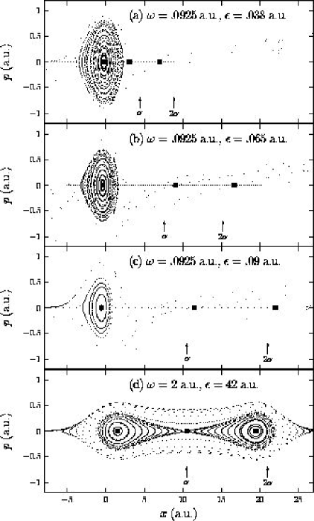
FIG. 1.: Strobe plots of the classical dynamics for the driven inverted Gaussian system. The initial conditions used to generate the plots all lie on the line $p=0$. $\alpha$ is the classical excursion parameter for a free electron the field. The locations of the periodic orbits (stable and unstable) are indicated by filled squares.

The quantum dynamics of this system has been the subject of several investigations during the past decade. The resonance states of this system were first calculated by Bardsley and Comella in 1989 [14]. More recent studies have focused on high-harmonic generation (HHG) in this system [15]. It is the findings of Ben-Tal, Moiseyev, and Kosloff [16], hereafter BMK, that have the most relevance to our work. They found that the number of resonance states in this system increased as the field strength was increased over a certain range. BMK attempt to explain the creation of new resonance states as the field strength is increased by analyzing the dynamics of the time-averaged system in a reference frame that oscillates with a free electron in the driving field, known as the Kramers-Henneberger or K-H frame [17]. They found qualitative agreement in that the number of bound states in the time-averaged potential increases as the field strength is increased. However, the quantitative agreement was not very good. This is not surprising since the time-averaged K-H description is only accurate for very high frequency driving fields. Since the frequency of the driving field used by BMK and in this work ($\omega=.0925$ a.u.) is lower than the frequency of motion for two of the bound states in the undriven system ($.4451$ a.u. and $.1400$ a.u.), the time-averaged K-H description is not quantitatively accurate. It is somewhat surprising that the time-averaged K-H description is qualitatively accurate because the classical motion of the system in the time-averaged K-H frame is stable while the classical motion of the true system is largely unstable. For $\alpha>1$ the time-averaged potential in the K-H frame is a double well with minima separated by approximately $2\alpha$. Motion in this double well would be quite different from that seen in the strobe plots in Fig. 1a-c (although it would closely resemble the motion shown in Fig. 1d, which is at a frequency that is high enough for the time-averaged K-H description to be valid). Our goal in this paper is to find an alternative explanation for the creation of resonance states as $\epsilon$ is increased in this system, an explanation that does not rely on the time-averaged K-H description.

III Complex Coordinate Scaling

In recent years the technique of complex coordinate scaling (CCS) has been used extensively in the study of open quantum systems. In this section we will review two versions of complex coordinate scaling (standard and exterior scaling) and show how these techniques can be used to compute the resonance states of an open, time-periodic system. Results from the standard and exterior scaling versions are compared, for both time-independent and time-dependent calculations.

A Standard complex coordinate scaling (CCS)

We first examine how the eigenvalues and eigenstates of a time-independent open system can be calculated using standard complex coordinate scaling (CCS), a technique that is examined in detail in [18, 19]. In this paper we will use a basis of particle-in-a-box states for our calculations. These states are defined by

$$\langle x|n\rangle=\sqrt{\frac{2}{L}}\sin\left(\frac{n\pi x}{L}-\frac{n\pi}{2}\right),$$ (4)

where $-L/2\leq x\leq L/2$. Calculations using CCS are performed just as they are in traditional quantum mechanics, except that the coordinate is scaled in the Hamiltonian so that $x\rightarrow xe^{i\theta}$ ($0\leq\theta<\pi/4$). Scaling the coordinate in this fashion allows us to represent resonance states, which are not in the Hilbert space, using square integrable eigenfunctions. As a result of this scaling the new time-independent Hamiltonian is

$$\tilde{H_{0}}=H_{0}(xe^{i\theta})=\frac{p^{2}e^{-2i\theta}}{2}-V_{0}\exp\left(-(xe^{i\theta}/a)\right).$$ (5)

The kinetic energy operator is easily evaluated using the basis states in Eq. 4. As long as our box is sufficiently large ($L>>2x_{0}/\sqrt{cos(2\theta)}$) we find that

$$\langle m|-V_{0}\exp\left(-(xe^{i\theta}/a)^{2}\right)|n\rangle=V(m+n)-V(|m-n|)$$ (6)

where

$$V(j)=\frac{V_{0}a\sqrt{\pi}e^{-i\theta}}{L}\exp\left(-\frac{j^{2}\pi^{2}a^{2}e^{-2i\theta}}{4L^{2}}\right)\cos\left(\frac{j\pi}{2}\right).$$ (7)

Once these matrix elements are calculated the $\tilde{H_{0}}$ matrix can be constructed. Diagonalizing $\tilde{H_{0}}$ yields the energy eigenvalues of the time-independent system as well as the eigenvectors

$$|\psi_{i}\rangle=\sum_{n=1}^{N}c_{ni}|n\rangle.$$ (8)

Fig. 2a shows the energy eigenvalues of $H_{0}$ calculated without complex scaling ($\theta=0$). The potential supports three bound states at $E=-0.4451$, $-0.1400$, and $-0.00014$ a.u. Without complex scaling all eigenvalues lie on the real axis. When the coordinate is scaled, though, the Hamiltonian becomes non-Hermitian and it is possible for eigenstates of the scaled system to have complex eigenvalues. This can be seen in Fig. 2b, which shows the eigenvalues calculated using CCS with $\theta=0.3$. The bound state eigenvalues remain on the real axis but the positive-energy continuum states are rotated into the lower half plane by an angle of $2\theta$. It is this rotation of the continuum that will allow us to identify resonances. No resonances exist for the system with Hamiltonian $\tilde{H_{0}}$, only bound states and a continuum of energy eigenvalues.

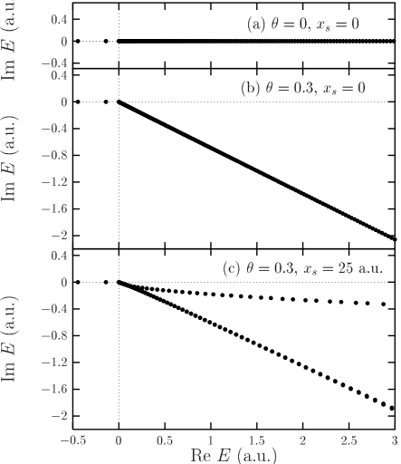
FIG. 2.: The complex-scaled energies of the undriven inverted Gaussian system. The unscaled energies are shown in (a), the CCS energies in (b), and the ECCS energies in (c). The bound states of the system have energies -0.4451, -0.1400, and -0.0001 a.u. All calculations were performed using a box size $L=200$ a.u. and 400 basis states.

B Exterior complex coordinate scaling

The basic idea of exterior complex coordinate scaling (ECCS) is to scale the $x$ coordinate by a factor $e^{i\theta}$ as in CCS, but only in the region $|x|\geq x_{s}$ where the potential is zero. Discontinuities at $\pm x_{s}$ are avoided by using a smooth scaling relation $x\rightarrow F(x)$, where

$$F(x)=x+(e^{i\theta}-1)\left[x+\frac{1}{2\lambda}\ln\left(\frac{\cosh(\lambda(x-x_{s}))}{\cosh(\lambda(x+x_{s}))}\right)\right]$$ (9)

with $\lambda=5$ a.u. and $x_{s}=25$ a.u. This exterior scaling method is given a thorough presentation in [19, 20]. Because the potential is zero in the region where the coordinate is scaled, the potential matrix elements can be calculated without any complex scaling (i.e. using Eq. 6 and 7, but with $\theta=0$). The scaled time-independent Hamiltonian then becomes $\tilde{H_{0}}=H_{0}+V_{CAP}$, where

$$V_{CAP}(x)=V_{0}(x)+V_{1}(x)\frac{\partial}{\partial x}+V_{2}(x)\frac{\partial^{2}}{\partial x^{2}}$$ (10)

acts as a complex absorbing potential. The coordinate-dependent factors in Eq. 10 are defined by

$$V_{0}(x)=\frac{1}{4}f^{-3}(x)\frac{\partial^{2}f}{\partial x^{2}}-\frac{5}{8}f^{-4}(x)\left(\frac{\partial f}{\partial x}\right)^{2},$$ (11)

$$V_{1}(x)=f^{-3}(x)\frac{\partial f}{\partial x},$$ (12)

and

$$V_{2}(x)=\frac{1}{2}(1-f^{-2}(x)),$$ (13)

where $f(x)=\partial F/\partial x$. Plots of $F(x)$, $V_{0}(x)$, $V_{1}(x)$, and $V_{2}(x)$ are shown in [19, 20].

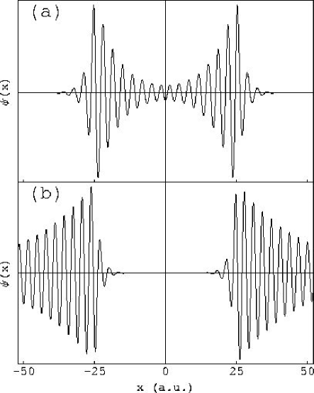
FIG. 3.: Wavefunctions of two ECCS continuum states. The state shown in (a) is a partially-scaled state whose eigenvalue is rotated by less than $2\theta$ from the real axis. The state in (b) is a fully-scaled state whose eigenvalue is rotated the full $2\theta$ from the real axis. The partially- scaled state is localized between $-x_{s}$ and $x_{s}$ ($x_{s}=25$ a.u.), while the fully-scaled state is almost excluded from this region. Both states are peaked near $\pm x_{s}$.

We will again use a basis of particle-in-a-box states to calculate $\tilde{H_{0}}$. Matrix elements for the potential energy term are calculated without any complex scaling, while the kinetic energy and $V_{CAP}$ matrix elements are calculated numerically. Diagonalizing $\tilde{H_{0}}$ gives the complex energy eigenvalues for the exterior scaled system, which are shown in Fig. 2c. Note that the bound state eigenvalues are still on the real axis and most of the continuum states have been rotated into the lower half plane by $2\theta$. However, several of the positive energy states have been rotated into the lower half plane by considerably less than $2\theta$. We refer to these as “partially scaled” continuum states. Fig. 3 shows the wavefunction of one fully scaled continuum state and one partially scaled continuum state. The partially scaled state is strongly peaked near $x=x_{s}$ and it is non-zero only within the region $-x_{s}\leq x\leq x_{s}$, while the fully scaled state is zero within this region. As $x_{s}$ is decreased toward $0$, the number of partially scaled states decreases. At $x_{s}=0$ the ECCS eigenvalues exactly match the CCS eigenvalues as expected.

Since we will want to examine the structure of the resonance wavefunctions in the periodically driven system it is important first to examine the structure of the eigenstates of $\tilde{H_{0}}$. We will examine the structure of the eigenstates of $\tilde{H_{0}}$ by calculating Husimi distributions [21] for each of the three bound states. An Husimi distribution is a quasi-probability distribution of a quantum state in the phase space. The Husimi distribution (HD) of a quantum wavefunction $\Psi(x)$ is defined as

$$G(x_{0},p_{0})=\left|\left(\frac{1}{\pi\sigma^{2}}\right)^{1/4}\int_{-\infty}^{-\infty}e^{-(x-x_{0})^{2}/2\sigma^{2}-ip_{0}x}\Psi(x)dx\right|^{2}.$$ (14)

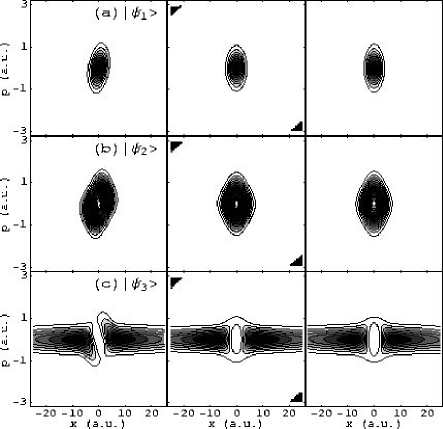
FIG. 4.: Husimi distributions of the bound states of the inverted Gaussian system. The distributions in the left column are of the CCS bound states. The distributions in the center column are CCS bound states rotated back into the real coordinate frame. The right column shows the distributions for the ECCS ($x_{s}=25$ a.u.) bound states. The scaling angle is $\theta=0.3$ for all plots.

Husimi distributions for the three bound states of $\tilde{H_{0}}$ are shown in Fig. 4. The left-hand column shows the HDs of the eigenstates, $\psi_{i}(x)$, of $\tilde{H_{0}}$ obtained using CCS. The center column shows the HDs for the eigenstates $\psi_{i}(xe^{i\theta})$, which is $\psi_{i}(x)$ rotated back to the real coordinate frame [22]. The right-hand column shows the HDs of the eigenstates that were calculated using ECCS. Note that the center and right-hand columns agree quite well, while the left-hand column shows significant differences. The Husimi distributions in the right-hand column match those that are found without complex scaling the Hamiltonian and hence they are the correct distributions. The distributions in the center column are correct except for the patches of black in the top-left and bottom-right corners. These patches show where the Husimi distribution blows up because the wavefunction is not square integrable.

C Floquet calculations

As we have seen, complex coordinate scaling can be used to calculate the first $N$ energy eigenstates of $\tilde{H_{0}}$. These eigenstates can then be used as a basis to compute the one-period time evolution (Floquet) matrix, $\hat{U}(T)$, for the driven system. This matrix is calculated by numerically integrating the time-dependent Schrödinger equation $N$ times from $t=0$ to $t=T=2\pi/\omega$ with initial conditions $|\Psi(t=0)\rangle=|\psi_{i}\rangle$, where $|\psi_{i}\rangle$ is the $i$th energy eigenstate of $\tilde{H_{0}}$. Diagonalization of this matrix gives the Floquet eigenvalues and eigenstates (in the basis of eigenstates of $\tilde{H_{0}}$).

The time-dependent Schrödinger equation for the driven inverted Gaussian system is

$$i\hbar\frac{\partial}{\partial t}|\Psi\rangle=\tilde{H_{0}}|\Psi\rangle-\frac{\epsilon}{\omega}\tilde{p}\sin(\omega t)|\Psi\rangle+\frac{\epsilon^{2}}{2\omega^{2}}\sin^{2}(\omega t)|\Psi\rangle$$ (15)

where $\tilde{p}$ is the complex scaled momentum operator. Since all computations are performed in a basis of eigenstates of $\tilde{H_{0}}$ we must first calculate the matrix elements of $\tilde{p}$. In calculating these matrix elements it is critical to recognize that $\tilde{H_{0}}$ is not a Hermitian matrix and thus its eigenvectors do not have the usual properties that eigenvectors of Hermitian matrices have. One cannot obtain the left eigenvectors of a non-Hermitian matrix simply by taking the complex conjugate of the right eigenvectors. In our case, $\tilde{H_{0}}$ is complex symmetric and the coefficients of the left eigenvectors are equal to (not complex conjugates of) the coefficients of the right eigenvectors, so

$$\langle\psi_{i}|=\sum_{n=1}^{N}c_{ni}\langle n|.$$ (16)

The normalization of the eigenvectors is also different. For our complex symmetric matrix the eigenvectors should be normalized so that the sum of the squares of the $c_{ni}$’s is $1$, rather than the sum of the absolute squares. With this in mind we can calculate the matrix elements for $\tilde{p}$ using

$$\langle\psi_{i}|\tilde{p}|\psi_{j}\rangle=\sum_{m=1}^{N}\sum_{n=1}^{N}c_{mi}c_{nj}\langle m|\tilde{p}|n\rangle.$$ (17)

The $\langle m|\tilde{p}|n\rangle$ are easy to calculate when CCS is used and $\tilde{p}$ is simply $pe^{-i\theta}$. However, when ECCS is used those matrix elements are calculated numerically using

$$\langle m|\tilde{p}|n\rangle=\frac{-i\hbar\pi n}{L^{2}}\left[P(m+n)+P(m-n)\right]$$ (18)

where

$$P(k)=\int_{-L/2}^{L/2}\sin\left(\frac{k\pi x}{L}-\frac{k\pi}{2}\right)f^{-1}(x)dx$$ (19)

and $f(x)$ is defined in Sec. III B.

By numerically integrating the Schrödinger equation over one cycle of the driving field we can construct the Floquet matrix as described above. This matrix is then numerically diagonalized to give the Floquet eigenvalues and eigenstates. Since the Floquet eigenstates are calculated in a basis of eigenstates of $\tilde{H_{0}}$ we can write them as

$$|q_{\beta}\rangle=\sum_{i=1}^{N}d_{i\beta}|\psi_{i}\rangle.$$ (20)

Because they are eigenstates of the one-period time evolution operator (Floquet matrix) we can write

$$\hat{U}(T)|q_{\beta}\rangle=e^{-iq_{\beta}T}|q_{\beta}\rangle$$ (21)

where $q_{\beta}$ is the quasienergy of the state $|q_{\beta}\rangle$. Because the Hamiltonian $\tilde{H_{0}}$ is not Hermitian, the time evolution operator is not unitary. This means that the Floquet eigenvalues do not necessarily have unit modulus, and thus the quasienergies $q_{\beta}$ are in general complex. We can write the quasienergies as $q_{\beta}=\Omega_{\beta}+i\Gamma_{\beta}/2$, where $\tau_{\beta}=1/\Gamma_{\beta}$ is the lifetime of the state $|q_{\beta}\rangle$. Resonance states are easily identified by plotting the Floquet eigenvalues, which we will denote as $\lambda_{\beta}=\exp(-iq_{\beta}T)$. Fig. 5 shows the Floquet eigenvalues calculated using both CCS and ECCS for the driven Gaussian system with $\omega=0.0925$ a.u. and $\epsilon=0.038$ a.u. The eigenvalues that were found with the CCS method form a well-defined spiral from the origin out to the edge of the unit circle. These states are indicated by filled circles in Fig. 5a. Resonance states are indicated by filled squares and lie off of the continuum spiral. The continuum spiral is not as well-defined when the ECCS method is used, as shown in Fig. 5b. However, only a few eigenvalues near the origin appear to fall out of the spiral. This could cause some difficulty in identifying broad (short-lived) resonances, but narrow (long-lived) resonances can still be easily identified. Fig. 5 shows that CCS and ECCS appear to give the same resonance eigenvalues.

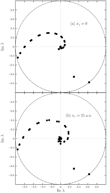
FIG. 5.: Floquet eigenvalues for the driven inverted Gaussian system with $\omega=0.0925$ a.u. and $\epsilon=0.038$ a.u. The eigenvalues calculated using CCS are shown in (a). In (b) the ECCS eigenvalues are shown. The scaling angle is $\theta=0.3$ for both sets of eigenvalues. Resonance states are indicated by filled squares, while continuum states are indicated by filled circles.

The resonance eigenvalues should be independent of the scaling angle $\theta$, while the continuum eigenvalues rotate around the origin as $\theta$ is changed. However, when calculations are performed using a finite basis the resonance eigenvalues will be weakly dependent upon $\theta$ [23]. To accurately determine the quasienergies (and hence the lifetimes) of these states it is important to optimize $\theta$ by finding the stationary point of each resonance eigenvalue as $\theta$ is changed. However, since our goal is not an accurate quantitative determination of eigenvalues or lifetimes but a qualitative understanding of the relationship between the quantum dynamics and the classical motion, it is not critical that $\theta$ be optimized for our calculations. Optimizing $\theta$ presents a problem in this type of study because the optimal value of $\theta$ is generally different for different resonance states. We wish to study all of the resonance states of the system at the same time and it is impossible to optimize $\theta$ for all resonance states within a single calculation of the Floquet matrix. We find that changing $\theta$ between $0.3$ and $0.7$ results in no visible change in the plots of the resonance eigenvalues. There is also no visible change in the Husimi distribution of the states. Not optimizing $\theta$ may lead to slight inaccuracies in the calculated lifetimes for the resonance states, but we find that the error in the lifetimes is no greater than $\pm 0.1T$ which is acceptable for our purpose here.

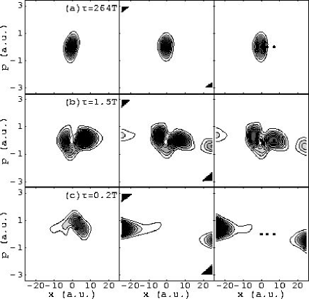
FIG. 6.: Husimi distributions of the resonance states at $\epsilon=0.038$ a.u. The left column shows the Husimi distributions of the states computed using CCS. The center column shows the distributions of the CCS states rotated back into the real coordinate frame. The right column shows the distributions of the ECCS states ($x_{s}=25$ a.u.). In the right-hand column the locations of the periodic orbits are indicated by filled circles and the contour plots have been lightened to allow the circles to show. The scaling angle is $\theta=0.3$ for all plots. The lifetimes for each state are given in units of the driving period $T=2\pi/\omega$.

In Figure 6 we show the Husimi distributions of the three resonance states indicated in Fig. 5. As in Fig. 4 the left-hand column shows CCS states, the middle column shows the rotated CCS states, and the right-hand column shows ECCS states. Again we find agreement between the middle and right-hand columns, while the left-hand column is inaccurate (as expected). Lifetimes of the three states are indicated in units of the driving period $T=2\pi/\omega$. Filled circles indicate the locations of the classical periodic orbits. The resonance state with the longest lifetime is almost indistinguishable from the ground state of the undriven system shown in Fig. 4a. The state shown in Fig. 6b has a much shorter lifetime and is beginning to elongate toward the positions of the unstable periodic orbits, with a peak of probability near the periodic orbit at ($x=6.98$ a.u., $p=0$). The state shown in Fig. 6c has a very short lifetime and its Husimi distribution is similar to that of a continuum state.

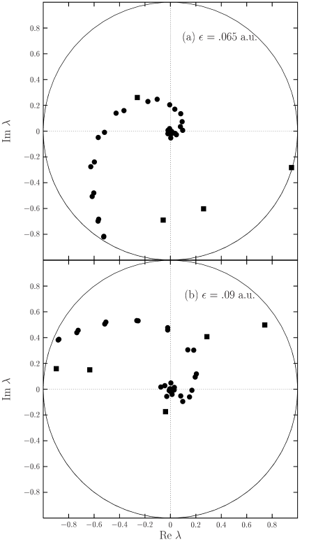
FIG. 7.: Floquet eigenvalues for $\omega=0.0925$ a.u. and two different field strengths. The eigenvalues are calculated using ECCS with $\theta=0.3$ and $x_{s}=25$ a.u. Resonance states are indicated by filled squares and continuum states by filled circles. At these higher field strengths the number of resonance states is greater than at $\epsilon=.038$ a.u.

IV Resonance creation and scarring

Because the rotated CCS states blow up for large $|x|$ we choose to perform the remainder of our calculations using ECCS only. As long as our unscaled region ($-x_{s}<x<x_{s}$) is large enough to contain the phase space region in which we are interested, we will not have to worry about any inaccuracy associated with the scaling procedures. We choose $x_{s}=25$ a.u. which is large enough to include the locations of the periodic orbits at all of the field strengths we study.

Figure 7 shows the Floquet eigenvalues for $\epsilon=0.065$ and $0.09$ a.u. Again, resonance states are indicated by filled squares while continuum states are indicated by filled circles. Comparing these plots with Fig. 5 we see that the number of resonance states increases as $\epsilon$ is increased, from only three at $\epsilon=0.038$ a.u. to five at $\epsilon=0.09$ a.u. This is in agreement with BMK [16]. In the classical system, however, the stable structure near $(x=0,p=0)$ gets smaller as $\epsilon$ is increased. If the resonance states were associated with this stable classical structure then some of the resonances should disappear as $\epsilon$ is increased. Instead, the opposite behavior is found. To find the explanation for the increase in the number of resonance states we examine the Husimi distributions of the resonance states indicated in Fig. 7.

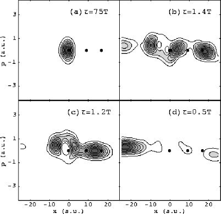
FIG. 8.: Husimi distributions for the four resonance states at $\epsilon=0.065$ a.u. Lifetimes for each state are given in units of the driving period $T=2\pi/\omega$. The locations of the periodic orbits are indicated by filled circles.

Figure 8 shows HDs for the four resonance states at $\epsilon=0.065$ a.u. Lifetimes for the states are indicated in units of the driving period and the positions of the periodic orbits are indicated by filled circles. The state with the longest lifetime looks very much like the ground state of the undriven system. The states shown in Figs. 8b and 8c show some similarities to the excited states of the undriven system, but they have both been elongated in the direction of the unstable periodic orbits. The state shown in Fig. 8b has a probability peak near the unstable periodic orbit at ($x=16.67$ a.u., $p=0$), while the state shown in Fig. 8c has a peak between the two unstable orbits. These two states appear to have become at least partially associated with the unstable periodic orbits. The state shown in Figure 8d is the newly created resonance and it has the shortest lifetime of the four. It has a modest peak near the periodic orbit at ($x=9.09$ a.u., $p=0$).

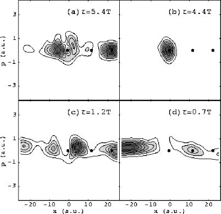
FIG. 9.: Husimi distributions for the four of the five resonance states at $\epsilon=0.09$ a.u. The resonance state with the shortest lifetime is not shown because its Husimi distribution is indistiguishable from that of a continuum state. Lifetimes for each state are given in units of the driving period $T=2\pi/\omega$. The locations of the periodic orbits are indicated by filled circles.

Figure 9 shows HDs for four of the five resonance states at $\epsilon=0.09$ a.u. The state that closely resembles the undriven ground state (Fig. 9b) no longer has the longest lifetime. Instead, the longest-lived state resembles the first excited bound state of $H_{0}$, but with additional peaks near the periodic orbits at $x=11.52$ a.u. and $x=22.04$ a.u. The state shown in Fig. 9d is similar to the state shown in Fig. 8d, but with a more prominent peak near the periodic orbit at $x=11.52$ a.u. Note that the lifetime of this state is also greater than that of the state shown in Fig. 8d.

At low values of $\epsilon$ all of the resonances have their probability concentrated near $(x=0,p=0)$. At these low values of $\epsilon$ the two unstable periodic orbits are located close to the stable orbit near $(x=0,p=0)$. If any resonance state was associated with the unstable periodic orbits at such low field strengths it would be difficult to tell from its Husimi distribution. As $\epsilon$ is increased the unstable periodic orbits move toward larger values of $x$ and some of the resonance states begin to spread in that direction as well. At moderate values of $\epsilon$ some states show peaks near the periodic orbit that is farthest from $(x=0,p=0)$, close to $x=2\alpha$. Only at high values of $\epsilon$ do we begin to see a state that is peaked on the unstable orbit that is closest to $(x=0,p=0)$, near $x=\alpha$. We believe that it is the association between the resonances and the unstable periodic orbits that explains the creation of resonance states as $\epsilon$ is increased. At low $\epsilon$ all three periodic orbits are too close together to support many quantum states because they all occupy essentially the same region of phase space. As $\epsilon$ is increased the unstable periodic orbits move away from the stable one and from each other. This allows quantum states to be associated with these unstable orbits without occupying the same region of phase space as the states associated with the stable orbit, so new resonance states are created. It is the scarring of resonance states on unstable periodic orbits of the classical system that accounts for the increase in the number of resonance eigenstates, even as the stable region in the classical phase space is diminished.

The behavior we see here would be unlikely to stabilize the ground state of the undriven system against ionization in a high intensity field. This is because the lifetime of the resonance state that seems most closely related to the ground state (shown in Figs. 6a, 8a, and 9b) decreases as $\epsilon$ is increased. However, the observed behavior could lead to stabilization for an excited state of the undriven system. The excited states have most of their probability away from $(x=0,p=0)$ and would thus overlap with resonance states that are not peaked at that point. Since these resonances grow in number and increase their lifetimes as $\epsilon$ is increased, an excited state of the undriven system may become stabilized against ionization as $\epsilon$ is increased.

V Avoided crossings between resonances

Avoided crossings between resonance eigenvalues have been identified in this system [15, 16]. Avoided crossings between Floquet eigenvalues play an important role in multi-photon ionization [24] and the delocalization of Floquet eigenstates [13]. In this section we investigate the quantum dynamics at one avoided crossing to determine if it leads to delocalization of the resonance eigenstates. Delocalization is closely related to ionization in these systems because long-lived resonance states can only exist if they are localized within the interaction region. If avoided crossings lead to delocalization they would also lead to a decrease in the lifetime, and eventually the destruction, of the resonance states.

Figure 10 shows the Floquet eigenvalues of three resonance states at several field strengths between $\epsilon=0.076$ and $0.085$ a.u. Two of these states (labeled $A$ and $B$ in Fig. 10 and indicated by filled circles and squares, respectively) are involved in a prominent avoided crossing at a field strength of about $\epsilon=0.0805$ a.u. The third resonance eigenvalue (labeled $C$ and indicated by filled triangles) passes close by the other two at this field strength, but it is not clear from Fig. 10 if that state is involved in the avoided crossing.

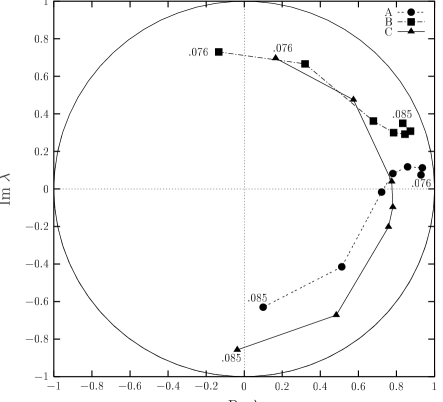
FIG. 10.: Floquet eigenvalues of three resonance states (labeled $A$, $B$, and $C$) that are involved in an avoided crossing around $\epsilon=0.0805$ a.u. The points show the eigenvalues for $\epsilon=.076,.078,.08,.0805,.081,.083,$ and $.085$ a.u. The numbers shown in the plot indicate the field strengths at the end points of each eigenvalue sequence. The lines are intended only as an aid to the eye.

To determine the effect of this avoided crossing on the resonance states we examine the Husimi distributions of the states $A$, $B$, and $C$ shown in Figure 11. As $\epsilon$ is increased from $0.078$ a.u. to $0.0805$ a.u. the states $A$ and $B$ undergo strong mixing with each other. When the field strength is increased to $0.083$ a.u. we find that states $A$ and $B$ have completely exchanged their structure. State $C$ does not appear to have any significant structural changes in this range of field strengths. However, it should be noted that state $C$ has a significant increase in its lifetime as $\epsilon$ is increased from $0.078$ a.u. to $0.083$ a.u. States $A$ and $B$ exchange lifetimes as well as structure, but the lifetimes of both states at $\epsilon=0.083$ a.u. are somewhat smaller than the corresponding lifetimes at $\epsilon=0.078$ a.u. It may be that state $C$ somehow gains stability at the expense of states $A$ and $B$, even though it does not appear to pick up any of the structure of those states. Note that there are slight differences between the Husimi distributions of states $A$ and $B$ at $\epsilon=0.073$ a.u. and the corresponding distributions at $\epsilon=0.083$ a.u., but these may be due to a small amount of mixing with state $C$ or with continuum states.

Figure 11 does not reveal any significant increase in the delocalization of any of the resonance states. It does indicate that an avoided crossing of this type might lead to changes in the lifetimes of the resonance states, but although two states have their lifetimes decreased the third has its lifetime increased. There is no clear indication that this type of avoided crossing contributes to the destruction of the resonance states that might prevent stabilization at very high intensities of the driving field. We expect that the destruction of resonance states occurs primarily as the result of coupling between a resonance state and the continuum rather than between resonance states [25].

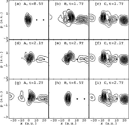
FIG. 11.: Husimi distributions for the states involved in the avoided crossings shown in Fig. 10. The labels $A$, $B$, and $C$ correspond to the labels in Fig. 10. Lifetimes for each state are given in units of the driving period $T=2\pi/\omega$. The top row (a-c) shows Husimi distributions for the three resonance states at $\epsilon=.078$ a.u. The second row (d-f) shows the distributions at $\epsilon=.0805$ a.u. The bottom row (g-i) shows the distributions at $\epsilon=.083$ a.u. States $A$ and $B$ appear to exchange their structure as they pass through the avoided crossing. State $C$ does not appear to undergo any major changes in its structure, but its lifetime increases dramatically as it passes through the avoided crossing. The locations of the periodic orbits at each field strength are indicated by filled circles.

Avoided crossings between resonance states may play an important role in other phenomena in this system. For example, it has been shown in bound systems that avoided crossings between Floquet eigenstates can result in increased high harmonic generation (HHG). Avoided crossings contribute to increased HHG in two ways. During the turn-on of a laser field avoided crossings can put the quantum system into a superposition of Floquet states that may emit radiation at higher frequencies than would be emitted by a single Floquet state [26]. Avoided crossings also contribute to HHG by spreading the Floquet states over a wider range of energy, thus allowing a single Floquet state to emit higher frequency radiation. For the type of avoided crossing observed here the states are only delocalized near the exact field strength at which the avoided crossing occurs, because at this field strength the Floquet states have mixed their structure [13]. At that particular field strength, though, this effect could lead to increased HHG. In fact, increased HHG has been observed in previous studies of the avoided crossings in this system [15].

VI Conclusion

We utilize the complex coordinate Floquet method (CCFM) to calculate resonances for an inverted Gaussian potential driven by a monochromatic field. As has been previously observed, we find that the number of resonance states increases as the field strength is increased. This behavior in the quantum system seems to be opposite to what is observed in the classical system, where the dynamics becomes increasingly unstable as the field strength is increased. An examination of the Husimi distributions of the resonance states in this system shows that the newly created resonances states are associated with unstable periodic orbits in the classical motion. This scarring of the eigenstates on unstable periodic orbits has been seen in other systems and it represents one of the most significant deviations of quantum dynamics from the corresponding classical dynamics. In this system, resonance eigenstates are scarred on unstable periodic orbits and the movement of the periodic orbits in the phase space allows for the creation of new resonance states as the field strength is increased. The creation of these new resonance states might help to stabilize the system against ionization in intense fields.

An avoided crossing between resonance states is closely examined and it is found that, although two states do exchange their structure during the avoided crossing, there is no significant delocalization of the resonance states as a result of this avoided crossing. Coupling to the continuum is more likely to destroy resonance states than is coupling between two resonance states. Avoided crossings of the type studied here, although they may not lead to faster ionization, could lead to many interesting effects such as increased high harmonic generation.

REFERENCES

- [1] Z. Chang, A. Rundquist, H. Wang, M. Murnane, and H. C. Kapteyn, Phys. Rev. Lett. 79, 2967 (1997).
- [2] J. H. Eberly, Q. Su, and J. Javanainen, J. Opt. Soc. Am. B 6, 1289 (1989).
- [3] L. E. Reichl, The Transition to Chaos In Conservative Classical Systems: Quantum Manifestations (Springer-Verlag, Berlin, 1983).
- [4] M. Pont and M. Gavrila, Phys. Rev. Lett. 65, 2362 (1990).
- [5] M. P. de Boer, J. H. Hoogenraad, R. B. Vrijen, R. C. Constantinescu, L. D. Noordam, and H. G. Muller, Phys. Rev. A 50, 4085 (1994)
- [6] C. O. Reinhold, J. Burgdörfer, M. T. Frey, and F. B. Dunning, Phys. Rev. Lett. 79, 5226 (1997).
- [7] W. Chism, D. Choi, and L. E. Reichl, Phys. Rev. A 61, 054702 (2000); R. Grobe and C. K. Law, Phys. Rev. A 44, R4114 (1991); F. Benvenuto, G. Casati, and D. L. Shepelyansky, Phys. Rev. A 47, R786 (1993); R. V. Jensen and B. Sundaram, Phys. Rev. A 47, R778 (1993); G. Casati, I. Guarneri, and G. Mantica, Phys. Rev. A 50, 5018 (1994).
- [8] J. H. Shirley, Phys. Rev. 138, B979 (1965); H. Sambe, Phys. Rev. A39, 2203 (1973).
- [9] S. Yoshida, C. O. Reinhold, P. Kristöfel, J. Burgdörfer, S. Watanabe, and F. B. Dunning, Phys. Rev. A 59, R4121 (1999).
- [10] E. B. Bogomolny, Physica D 31, 169 (1988); E. J. Heller, P. W. O’Connor, and J. Gehlen, Phys. Scr. 40, 354 (1989); E. Vergini and D. A. Wisniacki, Phys. Rev. E 58, R5225 (1998).
- [11] R. V. Jensen, M. M. Sanders, M. Saraceno, and B. Sundaram, Phys. Rev. Lett. 63, 2771 (1989); B. Sundaram and R. V. Jensen, Phys. Rev. A 47, 1415 (1993).
- [12] M. Latka, P. Grigolini, and B. J. West, Phys. Rev. A 50, 1071 (1994); M. Latka, P. Grigolini, and B. J. West, Phys. Rev. E 50, 596 (1994); Q. Jie, S.-J. Wang, and L.-F. Wei, Z. Phys. B 104, 373 (1997).
- [13] T. Timberlake and L. E. Reichl, Phys. Rev. A 59, 2886 (1999).
- [14] J. N. Bardsley and M. J. Comella, Phys. Rev. A 39, 2252 (1989).
- [15] N. Ben-Tal, N. Moiseyev, R. Kosloff, and C. Cerjan, J. Phys. B 26, 1445 (1993); N. Ben-Tal, N. Moiseyev, and R. Kosloff, Phys. Rev. A 48, 2437 (1993).
- [16] N. Ben-Tal, N. Moiseyev, and R. Kosloff, J. Chem. Phys. 98, 9610 (1993).
- [17] H. A. Kramers, Collected Scientific Papers (North-Holland, Amsterdam, 1956), p. 272; W. C. Henneberger, Phys. Rev. Lett. 52, 613 (1984).
- [18] W. P. Reinhardt, Ann. Rev. Phys. Chem. 33, 223 (1982).
- [19] N. Moiseyev, Phys. Rep. 302, 211 (1998).
- [20] N. Moiseyev, J. Phys. B 31, 1431 (1998).
- [21] K. Husimi, Proc. Phys. Math. Soc. Jpn. 22, 246 (1940); K. Takahashi, Prog. Theo. Phys. Supp. 98, 109 (1989).
- [22] I. Vorobeichik and N. Moiseyev, Phys. Rev. A 59, 1699 (1999).
- [23] O. E. Alon and N. Moiseyev, Phys. Rev. A 46, 3807 (1992); N. Lipkin, N. Moiseyev, and E. Brändas, Phys. Rev. A 40, 549 (1989).
- [24] Y. Gontier and M. Trahim, Phys. Rev. A 19, 264 (1979); C. R. Holt, M. G. Raymer, and W. P. Reinhardt, Phys. Rev. A 27, 2971 (1983).
- [25] T. Timberlake and L. E. Reichl (unpublished).
- [26] W. Chism, T. Timberlake, and L. E. Reichl, Phys. Rev. E 58, 1713 (1998).