Optimal States and Almost Optimal Adaptive Measurements for Quantum Interferometry

Abstract

We derive the optimal $N$-photon two-mode input state for obtaining an estimate $\phi$ of the phase difference between two arms of an interferometer. For an optimal measurement [B. C. Sanders and G. J. Milburn, Phys. Rev. Lett. 75, 2944 (1995)], it yields a variance $(\Delta\phi)^{2}\simeq\pi^{2}/N^{2}$, compared to $O(N^{-1})$ or $O(N^{-1/2})$ for states considered by previous authors. Such a measurement cannot be realized by counting photons in the interferometer outputs. However, we introduce an adaptive measurement scheme that can be thus realized, and show that it yields a variance in $\phi$ very close to that from an optimal measurement.

Interferometry is the basis of many high-precision measurements. The ultimate limit to the precision is due to quantum effects. This limit is most easily explored for a Mach-Zehnder interferometer (see Fig. 1, where $\Phi$ should be ignored for the moment). The outputs of this device can be measured to yield an estimate $\phi$ of the phase difference $\varphi$ between the two arms of the interferometer. It is well known that this can achieve the standard quantum limit for phase sensitivity of $(\Delta\phi)^{2}\simeq N^{-1}$ when an $N$-photon number state enters one input port. Several authors Caves ; Yurke ; Holland ; SandMil95 ; SandMil97 have proposed ways of reducing the phase variance to the Heisenberg limit of ${\sim}N^{-2}$. Here $N$ is the fixed total number of photons in the inputs fn1 .

Most of these proposals Caves ; Yurke ; Holland are limited in that they require that the phase difference $\varphi$ between the two arms be zero or very small in order to obtain the $N^{-2}$ scaling. Sanders and Milburn SandMil95 ; SandMil97 considered an ideal or canonical measurement, for which the $N^{-2}$ scaling is independent of $\varphi$. Unfortunately they do not explain how this measurement can be performed, and it can be shown BerWis01 that it cannot be realized by counting photons in the outputs of the interferometer. In this Letter we show that there is an experimentally realizable measurement scheme using photodetectors and feedback which is almost as good as the canonical measurement.

Before introducing our adaptive scheme, we find the optimal input states for the canonical interferometric measurements. These will then be used as the input states for our adaptive scheme, to demonstrate a $(\Delta\phi)^{2}$ scaling almost as good as $N^{-2}$. The optimal input states are interesting in themselves, in that they differ significantly from the input states considered in Refs. Caves ; Yurke ; Holland ; SandMil95 ; SandMil97 . In particular, our rigorous analysis shows that those non-optimal states, in fact, exhibit a worse scaling than the standard quantum limit of $N^{-1}$.

The canonical measurement.—Using the same notation as Sanders and Milburn SandMil95 , we designate the two annihilation operators for the two input modes as $\hat{a}$ and $\hat{b}$, and we use the Schwinger representation

$$\hat{J}_{x}=(\hat{a}^{\dagger}\hat{b}+\hat{a}\hat{b}^{\dagger})/2,~{}~{}~{}\hat{J}_{y}=(\hat{a}^{\dagger}\hat{b}-\hat{a}\hat{b}^{\dagger})/2i,$$ (1)

$$\hat{J}_{z}=(\hat{a}^{\dagger}\hat{a}-\hat{b}^{\dagger}\hat{b})/2,~{}~{}~{}\hat{J}^{2}=\hat{J}_{x}^{2}+\hat{J}_{y}^{2}+\hat{J}_{z}^{2}.$$ (2)

We use the notation $|{j\mu}\rangle_{z}$ for the common eigenstate of $\hat{J}_{z}$ and $\hat{J}^{2}$ with eigenvalues $\mu$ and $j(j+1)$, respectively. This state corresponds to Fock states with $j+\mu$ and $j-\mu$ photons entering ports $a$ and $b$, respectively.

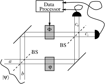
Figure 1: The Mach-Zehnder interferometer, with the addition of a controllable phase $\Phi$ in one arm. The unknown phase to be estimated is $\varphi$. Both beam splitters (BS) are 50:50.

From Ref. SandMil97 , the optimal probability operator measure (POM) for phase measurements is the canonical one,

$$\hat{E}(\phi)d\phi=\frac{2j+1}{2\pi}|{j\phi}\rangle\langle{j\phi}|d\phi,$$ (3)

where the phase states $|{j\phi}\rangle$ are defined in terms of the $\hat{J}_{y}$ eigenstates by $|{j\phi}\rangle=(2j+1)^{-1/2}\sum_{\mu=-j}^{j}e^{i\mu\phi}|{j\mu}\rangle_{y}$. In terms of the $\hat{J}_{y}$ eigenstates, the POM is

$$\hat{E}(\phi)d\phi=\frac{1}{2\pi}\sum_{\mu,\nu=-j}^{j}e^{i(\mu-\nu)\phi}|{j\mu}\rangle_{y}\langle{j\nu}|d\phi.$$ (4)

The POM defines the probability distribution for $\phi$, the best estimate for the interferometer phase $\varphi$, by

$$P(\phi)d\phi=\langle{\psi}|\hat{E}(\phi)|{\psi}\rangle d\phi.$$ (5)

Here $|{\psi}\rangle$ is the two-mode interferometer input state having $N=2j$ photons.

The optimal input state.—A short examination reveals that the canonical POM (4) has the same matrix elements as the POM for ideal measurements on a single mode with an upper limit of $N$ on the photon number. The optimal state in this case has been considered before SumPeg90 ; semiclass . Here we follow the procedure of Ref. semiclass , which minimizes the Holevo phase variance Hol84

$$(\Delta\phi)^{2}=V_{\phi}\equiv S_{\phi}^{-2}-1,$$ (6)

where $S_{\phi}\in[0,1]$ is the sharpness of the phase distribution, defined as

$$S_{\phi}\equiv\left|{\langle{e^{i\phi}}\rangle}\right|=\int_{0}^{2\pi}d\phi P(\phi)e^{i(\phi-\bar{\phi})},$$ (7)

where the “mean phase” $\bar{\phi}$ is defined so that $S_{\phi}$ is positive. The Holevo variance is the natural quantifier for dispersion in a cyclic variable. If the variance is small, then it is easy to show that

$$V_{\phi}\simeq\int_{0}^{2\pi}4\sin^{2}\left({\frac{\phi-\bar{\phi}}{2}}\right)P(\phi)d\phi,$$ (8)

from which the equivalence to the usual definition of variance for well-localized distributions is readily apparent.

Using the Holevo variance enables a simple analytic solution. The minimum variance is

$$\tan^{2}\left(\frac{\pi}{N+2}\right)=\frac{\pi^{2}}{(N+2)^{2}}+O(N^{-4}),$$ (9)

and the optimal state (chosen here to have a mean relative phase of zero) is

$$|{\psi_{\rm opt}}\rangle=\frac{1}{\sqrt{j+1}}\sum_{\mu=-j}^{j}\sin\left[\frac{(\mu+j+1)\pi}{2j+2}\right]|{j\mu}\rangle_{y}.$$ (10)

To obtain the state in terms of the eigenstates of $\hat{J}_{z}$, we use ${}_{y}\langle{j\mu}|{j\nu}\rangle_{z}=e^{i(\pi/2)(\nu-\mu)}I_{\mu\nu}^{j}(\pi/2)$, where SandMil95

$$I_{\mu\nu}^{j}(\pi/2) =2^{-\mu}\left[\frac{(j-\mu)!}{(j-\nu)!}\frac{(j+\mu)!}{(j+\nu)!}\right]^{1/2}P_{j-\mu}^{(\mu-\nu,\mu+\nu)}(0),$$

$$\textrm{for }\mu-\nu>-1,\;\;\mu+\nu>-1,$$ (11)

where $P_{n}^{(\alpha,\beta)}(x)$ are the Jacobi polynomials, and the other matrix elements are obtained using the symmetry relations $I_{\mu\nu}^{j}(\theta)=(-1)^{\mu-\nu}I_{\nu\mu}^{j}(\theta)=I_{-\nu,-\mu}^{j}(\theta)$.

An example of the optimal state for 40 photons is plotted in Fig. 2. This state contains contributions from all the $\hat{J}_{z}$ eigenstates, but the only significant contributions are from 9 or 10 states near $\mu=0$. The distribution near the center is fairly independent of photon number $N=2j$. To demonstrate this, the distribution near the center for 1200 photons is also shown in Fig. 2.

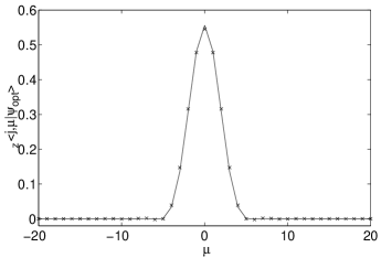
Figure 2: The coefficients ${}_{z}\langle{j\mu}|\psi_{\rm opt}\rangle$ for the state optimized for minimum phase variance under ideal measurements. All coefficients for a photon number of $2j=40$ are shown as the continuous line, and those near $\mu=0$ for a photon number of $2j=1200$ as crosses.

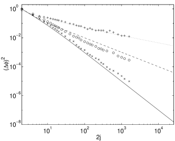
Figure 3: Variances in the phase estimate versus input photon number $2j$. The lines are exact results for canonical measurements on optimal states $|{\psi_{\rm opt}}\rangle$ (continuous line), on states with all photons incident on one input port $|{jj}\rangle_{z}$ (dashed line), and on states with equal photon numbers incident on both input ports $|{j0}\rangle_{z}$ (dotted line). The crosses are the numerical results for the adaptive phase measurement scheme on $|{\psi_{\rm opt}}\rangle$, and the plusses are those on a $|{j0}\rangle_{z}$ input state. The circles are numerical results for a nonadaptive phase measurement scheme on $|{\psi_{\rm opt}}\rangle$. All variances for the $|{j0}\rangle_{z}$ state are for phase modulo $\pi$.

In order to compare this state with $|{j0}\rangle_{z}$, where equal photon numbers are fed into both input ports (as considered in Refs. Holland ; SandMil95 ; SandMil97 ), the exact phase variance for this case was calculated for a range of photon numbers up to 25 600. Since the phase must be measured modulo $\pi$ for this state, rather than using the Holevo phase variance, we used the following measure for the dispersion:

$$(\Delta\phi)^{2}=V_{2\phi}/4=(|\langle{e^{2i\phi}}\rangle|^{-2}-1)/4,$$ (12)

where the expectation value is again determined using (5). The phase variances for this state and the optimal state are shown in Fig. 3. The exact Holevo phase variance of the state where all the photons are incident on one port, $|{jj}\rangle_{z}$, is also shown for comparison.

As can be seen, the phase variance for $|{j0}\rangle_{z}$ scales down with photon number much more slowly than the phase variance for optimal states fn2 , and even more slowly than the variance for $|{jj}\rangle_{z}$, which scales as $N^{-1}$. In fact, this figure shows that the phase variance for $|{j0}\rangle_{z}$ scales as $N^{-1/2}$, which agrees with what can be calculated from the asymptotic formula for $P(\phi)$ given in Ref. SandMil97 . This is a radically different result from the $N^{-2}$ scaling found in Refs. Holland ; SandMil95 ; SandMil97 . The state $(|{j0}\rangle_{z}+|{j1}\rangle_{z})/\sqrt{2}$, considered in Ref. Yurke , is even worse than the state $|{j0}\rangle_{z}$.

The reason for this discrepancy is that the results found in Refs. Holland ; SandMil95 ; SandMil97 are all based on the width of the central peak in the distribution, but the main contribution to the variance is from the tails of the distribution. This can be seen from the probability distribution multiplied by $\sin^{2}\phi$, since Eqs. (8) and (12) imply that $(\Delta\phi)^{2}\simeq\int\sin^{2}(\phi-\varphi)P(\phi)d\phi$. We plot this in Fig. 4 for $N=80$ and $\varphi=0$. In practice this means that the error in the phase will be small most of the time, but there will be a significant number of results with a large error.

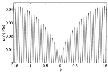
Figure 4: The canonical phase probability distribution for $|{j0}\rangle_{z}$ multiplied by $\sin^{2}\phi$ for $2j=80$ photons.

Adaptive measurements.—Although the quantum interferometry problem is now formally solved, this is of little practical use because (even if the optimal input states could be produced) it is not known how to implement the canonical measurement scheme. In particular, it is impossible to implement it by counting photons in the two output ports of the interferometer BerWis01 , as an experimenter would expect to do. Nevertheless, as we will show, it is possible to closely approximate the canonical measurement by counting output photons if one makes the measurement adaptive. The situation is as in Fig. 1. The unknown phase we wish to measure, $\varphi$, is in one arm of the interferometer, and we introduce a known phase shift, $\Phi$, into the other arm of the interferometer. After each photodetection we adjust this introduced phase shift in order to minimize the expected uncertainty of our best phase estimate after the next photodetection.

The annihilation operators $\hat{c}_{1}$ and $\hat{c}_{0}$ for the two output modes shown in Fig. 1 are related to the inputs by

$$\hat{c}_{u}(\varphi,\Phi)=\hat{a}\sin\frac{\varphi-\Phi+u\pi}{2}+\hat{b}\cos\frac{\varphi-\Phi+u\pi}{2}.$$

Before the $m$th photon has been detected, the phase $\Phi$ will be fixed to the value $\Phi_{m}$ by an adaptive algorithm to be specified later. Clearly the feedback loop which adjusts $\Phi_{m}$ must act much faster than the average time between photon arrivals. It is the ability to change $\Phi_{m}$ during the passage of a single (two-mode) pulse that makes photon counting measurements more general than a measurement of the output $\hat{J}_{z}$ considered in Refs. Yurke ; Holland .

An adjustable second phase $\Phi$ is of use even without feedback Hra96 . By setting

$$\Phi_{m}=\Phi_{0}+\frac{m\pi}{N},$$ (14)

where $\Phi_{0}$ is chosen randomly, an estimate $\phi$ of $\varphi$ can be made with an accuracy independent of $\varphi$. However, as we will show, this phase estimate has a variance scaling as $O(N^{-1})$ rather than $O(N^{-2})$.

Let us denote the result $u$ from the $m$th detection as $u_{m}$ (which is 0 or 1 according to whether the photon is detected in mode $c_{0}$ or $c_{1}$), and the measurement record up to and including the $m$th detection as the binary string $n_{m}\equiv u_{m}\cdots u_{2}u_{1}$. The input state after $m$ detections will be a function of the measurement record and $\varphi$, and we denote it as $|{\tilde{\psi}(n_{m},\varphi)}\rangle$. It is determined by the initial condition $|{\tilde{\psi}(n_{0},\varphi)}\rangle=|{\psi}\rangle$ and the recurrence relation

$$|{\tilde{\psi}(u_{m}n_{m-1},\varphi)}\rangle=\hat{c}_{u_{m}}(\varphi,\Phi_{m})\frac{|{\tilde{\psi}(n_{m-1},\varphi)}\rangle}{\sqrt{N+1-m}}.$$ (15)

These states are unnormalized, and their norm represents the probability for the record $n_{m}$, given $\varphi$,

$$P(n_{m}|\varphi)=\langle{\tilde{\psi}(n_{m},\varphi)}|{\tilde{\psi}(n_{m},\varphi)}\rangle.$$ (16)

Thus the probability of obtaining the result $u_{m}$ at the $m$th measurement, given the previous results $n_{m-1}$, is

$$P(u_{m}|\varphi,n_{m-1})=\frac{\langle{\tilde{\psi}(u_{m}n_{m-1},\varphi)}|{\tilde{\psi}(u_{m}n_{m-1},\varphi)}\rangle}{\langle{\tilde{\psi}(n_{m-1},\varphi)}|{\tilde{\psi}(n_{m-1},\varphi)}\rangle}.$$ (17)

Also, the posterior probability distribution for $\varphi$ is

$$P(\varphi|n_{m})={\cal N}_{m}(n_{m})\langle{\tilde{\psi}(n_{m},\varphi)}|{\tilde{\psi}(n_{m},\varphi)}\rangle,$$ (18)

where ${\cal N}_{m}(n_{m})$ is a normalization factor. To obtain this we have used Bayes’ theorem assuming a flat prior distribution for $\varphi$ (that is, an initially unknown phase). A Bayesian approach to interferometry has been considered previously, and even realized experimentally Hra96 . However, this was done only with nonadaptive measurements and with all particles incident on one input port.

With this background, we can now specify the adaptive algorithm for $\Phi_{m}$. The sharpness of the distribution after the $m$th detection is given by

$$S_{\varphi}(u_{m}n_{m-1})=\left|\int_{0}^{2\pi}P(\varphi|u_{m}n_{m-1})e^{i\varphi}d\varphi\right|.$$ (19)

We choose the feedback phase before the $m$th detection, $\Phi_{m}$, to maximize the sharpness. Since we do not know $u_{m}$ beforehand, we weight the sharpnesses for the two alternative results by their probability of occurring based on the previous measurement record. Therefore the expression we maximize is

$$M(\Phi_{m}|n_{m})=\sum_{u_{m}=0,1}P(u_{m}|n_{m-1})S_{\varphi}(u_{m}n_{m-1}).$$ (20)

Using Eqs. (17), (18), and (19), and ignoring the constant ${\cal N}_{m}(n_{m})$, the maximand can be rewritten as

$$\sum_{u_{m}=0,1}\left|\int_{0}^{2\pi}\langle{\tilde{\psi}(u_{m}n_{m-1},\varphi)}|{\tilde{\psi}(u_{m}n_{m-1},\varphi)}\rangle e^{i\varphi}d\varphi\right|.$$ (21)

The controlled phase $\Phi_{m}$ appears implicitly in (21) through $\hat{c}_{u_{m}}(\varphi,\Phi_{m})$ in (Optimal States and Almost Optimal Adaptive Measurements for Quantum Interferometry), which appears in the recurrence relation (15). The maximizing solution $\Phi_{m}$ can be found analytically, but we will not exhibit it here.

The final part of the adaptive scheme is choosing the phase estimate $\phi$ of $\varphi$ from the complete data set $n_{N}$. To maximize ${\rm Re}[\langle{e^{i(\phi-\varphi)}}\rangle]$ (that is, to minimize the deviation of $\phi$ from $\varphi$), we choose $\phi$ to be the mean of the posterior distribution $P(\varphi|n_{N})$, which from Eq. (18) is

$$\phi=\arg\int_{0}^{2\pi}\langle{\tilde{\psi}(n_{N},\varphi)}|{\tilde{\psi}(n_{N},\varphi)}\rangle e^{i\varphi}d\varphi.$$ (22)

We can determine the approximate phase variance $(\Delta\phi)^{2}$ under this adaptive scheme using a stochastic method. The phase $\varphi$ is taken to be zero, which leads to no loss of generality since the initial controlled phase $\Phi_{1}$ is chosen randomly. The measurement results are determined randomly with probabilities determined using $\varphi=0$, and the final estimate $\phi$ determined as above. From Eq. (6), an ensemble $\{\phi_{\mu}\}_{\mu=1}^{M}$ of $M$ final estimates allows the phase variance to be approximated by $(\Delta\phi)^{2}\simeq-1+|{M}^{-1}\sum_{\mu=1}^{M}e^{i\phi_{\mu}}|^{-2}$. It is also possible to determine the phase variance exactly by systematically going through all the possible measurement records and averaging over $\Phi_{1}$. This method is feasible only for photon numbers up to 20 or 30, however.

The results of using this adaptive phase measurement scheme on the optimal input states determined above are shown in Fig. 3. The phase variance is very close to the phase variance for ideal measurements, with scaling very close to $N^{-2}$. The phase variances do differ relatively more from the ideal values for larger photon numbers, however, indicating a scaling slightly worse than $N^{-2}$. It is possible that the actual scaling is $\log N/N^{2}$, as is the case for optimal single-mode adaptive phase measurements based on dyne detection fullquan ; unpub . For comparison, we also show the variance from the nonadaptive phase measurement defined by Eq. (14). As is apparent, this has a variance scaling as $N^{-1}$. Finally, the results for $|{j0}\rangle_{z}$ input states with this adaptive phase measurement scheme (modified to estimate $\varphi$ modulo $\pi$, as we must for these states) are also shown. The variances are again close to those for ideal measurements, scaling as $N^{-1/2}$.

To conclude, we have shown that although the $|{j0}\rangle_{z}$ input states considered by previous authors do not give a phase variance that scales as $1/N^{2}$ under ideal measurements, it is straightforward to derive optimal input states that do give this scaling. These states require significant contributions from only 9 or 10 $\hat{J}_{z}$ eigenstates (photon eigenstates for the two input modes). We have also demonstrated a practical measurement scheme (i.e., one based on photodetection of the output modes) to approximate ideal measurements. This scheme, which uses feedback, allows phase measurements with a variance scaling close to $1/N^{2}$ with optimized input states.

References

- (1) C. M. Caves, Phys. Rev. D 23, 1693 (1981).
- (2) B. Yurke, S. L. McCall, and J. R. Klauder, Phys. Rev. A 33, 4033 (1986).
- (3) M. J. Holland and K. Burnett, Phys. Rev. Lett. 71, 1355 (1993).
- (4) B. C. Sanders and G. J. Milburn, Phys. Rev. Lett. 75, 2944 (1995).
- (5) B. C. Sanders, G. J. Milburn, and Z. Zhang, J. Mod. Opt. 44, 1309 (1997).
- (6) Except for Ref. Caves , the above proposals have involved input states where the total number of photons is fixed. For simplicity, we follow this convention.
- (7) We have found that for and our feedback scheme as applied to optimum input states is globally optimum, and also that the phase variance is above the canonical phase variance. This demonstrates that canonical measurements cannot be realized by counting photons in the interferometer outputs, even if feedback is allowed.
- (8) G. S. Summy and D. T. Pegg, Opt. Commun. 77, 75 (1990).
- (9) H. M. Wiseman and R. B. Killip, Phys. Rev. A 56, 944 (1997).
- (10) A. S. Holevo, Springer Lecture Notes Math. 1055, 153 (1984).
- (11) The phase variance starts out less than that for the optimum state, but this is merely due to using a slightly different measure of the variance.
- (12) Z. Hradil et al., Phys. Rev. Lett. 76, 4295 (1996).
- (13) H. M. Wiseman and R. B. Killip, Phys. Rev. A 57, 2169 (1998).
- (14) D. W. Berry and H. M. Wiseman, Phys. Rev. A63, 013813 (2001).