Quantum Magic Bullets via Entanglement

Abstract

Two particles that are entangled with respect to continuous variables such as position and momentum exhibit a variety of nonclassical features. First, measurement of one particle projects the other particle into the state that is the complex conjugate of the state of the first particle, i.e., measurement of one particle projects the other particle into the time-reversed state. Second, continuous-variable entanglement can be used to implement a quantum “magic bullet”: when one particle manages to pass through a scattering potential, then no matter how low the probability of this event, the second particle will also pass through a related scattering potential with probability one. This phenomenon is investigated in terms of the original EPR state, and experimental realizations are suggested in terms of entangled photon states.

I Introduction

Entanglement is a peculiar quantum phenomenon in which two quantum systems exhibit a greater degree of correlation than is permitted classically. Entanglement has been shown to be a highly useful effect for quantum computation and quantum communications, see [1] for a recent review. One of the earliest and most striking pictures of entanglement was given by Einstein, Podolsky, and Rosen (EPR) in their original paper on entangled states [2]. In contrast with the majority of subsequent work, the original EPR paper concentrated on entanglement of continuous variables, position and momentum. Although most recent work on entanglement has focused on discrete systems such as quantum bits or qubits, experimental demonstration of continuous-variable teleportation via entanglement [3], theoretical constructions of analog quantum error-correcting codes [4, 5, 6], and methods for universal quantum computation over continuous variables [7] suggest that the original EPR state is well-worth revisiting.

This paper shows that entanglement of continuous variables exhibits several significant properties in the context of scattering theory. Consider two particles that are entangled in terms of continuous variables such as position and momentum. Measurement of one particle can be shown to project the other particle into the complex conjugate, or time-reversed state. This fact has the following consequence. Consider a potential barrier put in the path of the first particle that reflects some states and transmits other states with probability one (such a barrier can be thought of as a generalized filter). Then there is a related potential barrier for the second particle—corresponding to the time-reversed scattering matrix for the first potential—such that if the first particle is transmitted through its barrier, the second particle will be transmitted through its barrier with probability one. We call this effect, a quantum “magic bullet.” This paper presents a theoretical exposition of the magic bullet effect both in terms of the original EPR state and in terms of entangled photons, and proposes experimental realizations of quantum magic bullets.

II EPR-State Magic Bullets

First, let us revisit the original Einstein-Podolsky-Rosen state. Suppose that a particle with zero momentum decays into two particles at time $t=0$. The particles have position eigenstates $|x\rangle_{j}$, and momentum eigenstates $|p\rangle_{j}=(1/\sqrt{2\pi\hbar})\int_{-\infty}^{\infty}e^{ipx/\hbar}|x\rangle_{j}dx$, where $j=1,2$. (Like EPR, we restrict our attention to a one-dimensional system: the multi-dimensional generalization is straightforward.) Immediately after the initial particle’s decay, the joint state of the two new particles is

$$|\psi\rangle_{\rm EPR}=\int_{-\infty}^{\infty}|x\rangle_{1}|x\rangle_{2}\,dx=\int_{-\infty}^{\infty}|p\rangle_{1}|-p\rangle_{2}\,dp.$$ (1)

These two particles are thus perfectly correlated in position, and also perfectly anticorrelated in momentum. It was this dual correlation that Einstein, Podolsky and Rosen suggested was incompatible with the classical notion of reality: the EPR state seems to allow each particle to be in an eigenstate of two noncommuting observables.

Irrespective of interpretations of quantum mechanics (which are notoriously slippery), the EPR state exhibits the following property. We expand $|\psi\rangle_{\rm EPR}$ in terms of an arbitrary orthonormal basis $\{|\phi_{z}\rangle\}$, indexed by a continuous parameter $z$, obtaining $|\phi_{z}\rangle_{j}=\int\phi_{z}(x)|x\rangle_{j}dx$, where $\phi_{z}(x)=\langle x|\phi_{z}\rangle$. Then, recalling that $|x\rangle^{*}=|x\rangle$, we have

$$|\psi\rangle_{\rm EPR}=\int|\phi_{z}\rangle_{1}|\phi_{z}\rangle^{*}_{2}\,dz.$$ (2)

Suppose that a measurement of an operator with eigenstates $|\phi_{z}\rangle_{1}$ is made on the first particle. It is immediately seen that if this measurement reveals the first particle to be in the state $|\phi_{z}\rangle_{1}$, the second particle is then in the complex conjugate state $|\phi_{z}\rangle^{*}_{2}$.

Complex conjugation in quantum mechanics is equivalent to time reversal. If a particle evolves according to a Hamiltonian $\hat{H}$, so that an initial state $|\phi\rangle$ at $t=0$ evolves into the state $|\phi(t)\rangle=e^{-i\hat{H}t/\hbar}|\phi\rangle$ for $t>0$, then taking the complex conjugate gives the state $e^{i\hat{H}^{*}t/\hbar}|\phi\rangle^{*}$, viz., the complex conjugate of the evolved state is the complex conjugate of the initial state evolved backward in time ($t\rightarrow-t$) according to the time-reversed Hamiltonian $\hat{H}^{*}$. If $\hat{H}$ is real, i.e., time-reversal invariant (as is the case for almost all fundamental Hamiltonians, with the notable exception of the $K^{0}$ meson), then the energy eigenfunctions of $\hat{H}$ can be taken to be real, because $\hat{H}|E\rangle=E|E\rangle$ implies $\hat{H}|E\rangle^{*}=E|E\rangle^{*}$. Suppose that both particles in the EPR state are subjected to a time-reversal invariant Hamiltonian $\hat{H}$. Over time $t$, the state $|\psi\rangle_{\rm EPR}$ evolves into

$$|\psi(t)\rangle_{\rm EPR}\equiv\int e^{-i\hat{H}t/\hbar}|\phi_{z}\rangle_{1}e^{-i\hat{H}t/\hbar}|\phi_{z}\rangle^{*}_{2}\,dz=\int|\phi_{z}(t)\rangle_{1}|\phi_{z}(-t)\rangle^{*}_{2}\,dz.$$ (3)

The state of the first particle at time $t$ is thus perfectly correlated with a state that is the complex conjugate of that particle’s state at time $-t$: the second particle is in the time-reversed state of the first.

The EPR state also exhibits interesting scattering properties. Suppose that the first particle is subjected to a time-reversal invariant Hamiltonian corresponding to a unitary scattering matrix $\hat{S}(t)=e^{-i\hat{H}t/\hbar}$. Note that $\hat{S}^{*}(t)=\hat{S}^{\dagger}(t)=\hat{S}^{-1}(t)$. After the particle is scattered, let us make a projective measurement on it, corresponding to the Hermitian operator $\hat{O}=\sum_{o}o\hat{P}_{o}$, where $o$ is real and $\hat{P}_{o}=\hat{P}^{2}_{o}$ is the projection operator on the eigenspace corresponding to $o$. Now suppose that the second particle is subjected to the inverse scattering operation $\hat{S}^{*}(t)$, and that the conjugate measurement $\hat{O}^{*}=\sum_{o}o\hat{P}_{o}^{*}$ is made on this particle. Then the results of the two measurements will be perfectly correlated: a result of $o$ for the first particle will be accompanied by a result $o$ for the second particle. That is, if the first particle passes through a given scattering potential, the second particle passes through the time-reversed potential with probability one, regardless of how unlikely it was for the first particle to have breached its barrier. We call this effect a quantum magic bullet.

The magic bullet effect can be implemented in other ways as well. For example, suppose that it is possible to conjugate the phase of the second particle (for example, by sending it off a phase-conjugate mirror) at time $t$. The phase conjugation effectively performs a spin echo on the particle, resulting in the state $\int|\phi_{z}(t)\rangle_{1}|\phi_{z}(-t)\rangle_{2}\,dz$. The second particle now performs the same dynamics as the first particle, but with a time lag of $2t$. In particular, if the first particle manages to pass through a generalized filter, then the second particle will pass through the same filter with probability one $2t$ seconds later.

Quantum magic bullets can have many manifestations. We now turn to examples of quantum magic bullets that can be constructed using nonlinear optics.

III Field-Quadrature Magic Bullets

Parametric interactions in $\chi^{(2)}$ crystals have proved to be rich sources of quantum light-beam phenomena, see [8, 9] for a unified treatment of a wide variety of such effects, including quadrature-noise squeezing, nonclassical twin-beam production, nonclassical fourth-order interference, and polarization-entangled photon-pair production. All these phenomena originate from the same fundamental physics: in a $\chi^{(2)}$ material pumped by a strong beam at frequency $\omega_{P}$ and wave vector ${\bf k}_{P}$, a single pump photon is converted into a pair of photons—one signal ($S$) and one idler ($I$)—subject to the energy- and momentum-conservation conditions, i.e., $\omega_{S}+\omega_{I}=\omega_{P}$ and ${\bf k}_{S}+{\bf k}_{I}={\bf k}_{P}$, respectively.

We shall use the continuous-wave, type-II phase matched, doubly-resonant optical parametric amplifier (OPA)—with vacuum-state signal and idler inputs—as the basis for all of the optical magic-bullet realizations to be discussed. This OPA arrangement, shown schematically in Fig. 1, produces signal and idler outputs with orthogonal polarizations, well-defined spatial modes, and fluorescence bandwidths in the MHz to GHz range. As in [9], we shall assume that the signal and idler linewidths are identical, that there are no losses in the OPA cavity, and that there is no depletion of nor excess noise on the pump beam. The positive-frequency, photon-units field operators for the excited output polarizations of the signal and idler, $\hat{E}_{S}(t)$ and $\hat{E}_{I}(t)$, are then conveniently expressed in terms of their respective fluorescence center frequencies, $\omega_{S}$ and $\omega_{I}$, and their complex envelopes via, $\hat{E}_{j}(t)=\hat{A}_{j}(t)e^{-i\omega_{j}t}$, for $j=S,I$. The full, multi-mode, joint state of these output signal and idler fields is known to be a stationary, entangled, Gaussian pure state that is completely characterized by the following normally-ordered (fluorescence) and phase-sensitive spectra [9]:

$$S^{(n)}(\omega) \equiv \int_{-\infty}^{\infty}\langle\hat{A}_{S}^{\dagger}(t+\tau)\hat{A}_{S}(t)\rangle e^{-i\omega\tau}\,d\tau$$ (4)

$$= \int_{-\infty}^{\infty}\langle\hat{A}_{I}^{\dagger}(t+\tau)\hat{A}_{I}(t)\rangle e^{-i\omega\tau}\,d\tau=\left|\frac{\displaystyle 2G}{\displaystyle 1-G^{2}-(\omega/\Gamma)^{2}-2i\omega/\Gamma}\right|^{2},$$ (5)

$$S^{(p)}(\omega) \equiv \int_{-\infty}^{\infty}\langle\hat{A}_{S}(t+\tau)\hat{A}_{I}(t)\rangle e^{-i\omega\tau}\,d\tau=\frac{\displaystyle 2G[1+G^{2}+(\omega/\Gamma)^{2}]}{\displaystyle|1-G^{2}-(\omega/\Gamma)^{2}-2i\omega/\Gamma|^{2}}.$$ (6)

Here, $G^{2}$ is the OPA pump power, normalized to the threshold power for oscillation, and $\Gamma$ is the cavity-loss rate.

To establish an analogy between the multi-mode signal and idler fields and the two-particle EPR state, let us consider an arbitrary pair of entangled single-frequency modes, namely, the signal beam at frequency $\omega_{S}+\Delta\omega$ and the idler beam at frequency $\omega_{I}-\Delta\omega$. The joint signal$\times$idler state for these two modes has the number-ket representation,

$$|\psi\rangle_{SI}=\sum_{n=0}^{\infty}\sqrt{\frac{\displaystyle\bar{N}^{n}}{\displaystyle(\bar{N}+1)^{n+1}}}\,|n\rangle_{S}|n\rangle_{I},$$ (7)

where $\bar{N}=S^{(n)}(\Delta\omega)$ is the average number of photons per mode. Individually, each mode (signal and idler) is in a chaotic (Bose-Einstein) state, but their photon numbers are perfectly correlated. We shall return to this photon-pair property in the sections to follow. Our present course is to connect this signal$\times$idler state to the EPR state. For that purpose we need the field-quadrature representation for $|\psi\rangle_{SI}$.

The real and imaginary parts of a photon annihilation operator, $\hat{a}$, i.e, its quadrature components $\hat{a}_{1}\equiv\mbox{Re}(\hat{a})$ and $\hat{a}_{2}\equiv\mbox{Im}(\hat{a})$, behave like normalized versions of position and momentum. In particular, the $\hat{a}_{1}$ eigenkets, $|\alpha_{1}\rangle$, are related to the $\hat{a}_{2}$ eigenkets, $|\alpha_{2}\rangle$, by Fourier transformation, $|\alpha_{2}\rangle=(1/\sqrt{\pi})\int_{-\infty}^{\infty}e^{2i\alpha_{2}\alpha_{1}}|\alpha_{1}\rangle\,d\alpha_{1}$. The joint signal$\times$idler state given in Eq. 7 takes the following form, when written in the field-quadrature representation generated by the eigenkets of $\hat{a}_{S_{1}}$ and $\hat{a}_{I_{1}}$,

$$|\psi\rangle_{SI}=\int_{-\infty}^{\infty}\int_{-\infty}^{\infty}\psi(\alpha_{S_{1}},\alpha_{I_{1}})|\alpha_{S_{1}}\rangle_{S}|\alpha_{I_{1}}\rangle_{I}\,d\alpha_{S_{1}}\alpha_{I_{1}},$$ (8)

with

$$\psi(\alpha_{S_{1}},\alpha_{I_{1}})\equiv\exp\!\left[-(1+2\bar{N})\alpha_{S_{1}}^{2}+4\sqrt{\bar{N}(\bar{N}+1)}\,\alpha_{S_{1}}\alpha_{I_{1}}-(1+2\bar{N})\alpha_{I_{1}}^{2}\right]/\sqrt{\pi/2}.$$ (9)

Equations 8 and 9 are not identical to the EPR state, Eq. 1, but they do embody a nonclassical continuous-variable correlation. Optical homodyne detection [10] can be used to perform the $\hat{a}_{S_{1}}$ and $\hat{a}_{I_{1}}$ measurements. When such measurements are made on the state $|\psi\rangle_{SI}$, the unconditional (marginal) statistics for the $\hat{a}_{S_{1}}$ and $\hat{a}_{I_{1}}$ observations are identical: their individual outcomes are Gaussian random variables, each with mean zero and variance $(1+2\bar{N})/4$. It is the joint statistics of these two measurements that reveals pure quantum behavior. In particular, if we are given that the outcome of the $\hat{a}_{S_{1}}$ measurement is $\alpha_{S_{1}}$, then the conditional statistics of the $\hat{a}_{I_{1}}$ measurement remain Gaussian, but with conditional mean $[\sqrt{4\bar{N}(\bar{N}+1)}/(1+2\bar{N})]\alpha_{S_{1}}$ and conditional variance $1/4(1+2\bar{N})$. Thus, when $\bar{N}\geq 1$ there is a strong sub-shot-noise correlation between these signal-beam and idler-beam homodyne measurements: the conditional variance is substantially below that coherent-state (shot-noise) level of 1/4. Moreover, as $\bar{N}\longrightarrow\infty$, the state $|\psi\rangle_{SI}$ approaches a normalized version of the EPR state, as can be seen from rewriting $\psi(\alpha_{S_{1}},\alpha_{I_{1}})$ as follows:

$$\psi(\alpha_{S_{1}},\alpha_{I_{1}}) = \frac{\displaystyle\exp\!\left(-\frac{\displaystyle\alpha_{{S}_{1}}^{2}}{\displaystyle 1+2\bar{N}}\right)}{\displaystyle[\pi(1+2\bar{N})/2]^{1/4}}\frac{\displaystyle\exp\!\left[-(1+2\bar{N})\left(\alpha_{{I}_{1}}-\frac{\displaystyle\sqrt{4\bar{N}(\bar{N}+1)}}{\displaystyle 1+2\bar{N}}\alpha_{{S}_{1}}\right)^{2}\right]}{\displaystyle[\pi/2(1+2\bar{N})]^{1/4}}$$ (10)

$$\longrightarrow \frac{\displaystyle 1}{\displaystyle(\pi\bar{N})^{1/4}}\delta(\alpha_{I_{1}}-\alpha_{S_{1}}),\quad\mbox{as $\bar{N}\longrightarrow\infty$.}$$ (11)

Experimental demonstrations of this signal/idler homodyne correlation have already been reported [11, 12], although for optical parametric oscillators (OPOs)—in which the strong mean fields arising from above-threshold OPA operation act as homodyne-detection local oscillators—rather than for OPAs. An example of such data, obtained from a triply-resonant optical parametric oscillator [13], is shown in Fig. 2. The upper trace shows the shot-noise level and the lower trace shows the signal-minus-idler intensity difference for frequency detunings, $\Delta\omega/2\pi$, ranging from 2 to 6 MHz. The $>5$ dB noise reduction in the signal-minus-idler intensity difference is a manifestation of the nonclassical correlation cited above for the OPA field quadratures.

IV Photon-Pair Magic Bullets

Most entanglement experiments that rely on parametric optical interactions draw upon the photon-pair property exhibited in Eq. 7. Moreover, these experiments—which employ non-resonant, parametric downconverters rather than doubly-resonant optical parametric amplifiers—are carried out at extremely low photon fluxes. In this regime, a $T$-sec-long photon-counting measurement (on either the signal or idler beam) will yield zero counts with near-unity probability $1-p$, and one count with probability $p$; the probability of multiple counts at such low fluxes is negligible. Photon-pair creation within the $\chi^{(2)}$ medium is nearly instantaneous, but, for our doubly-resonant OPA, the time correlation between signal and idler photons in the output beams is smeared out to several cavity lifetimes. Thus, to represent the OPA version of low-flux photon-pair generation, we decompose $\hat{E}_{S}(t)$ and $\hat{E}_{I}(t)$—on a photon-counting interval $[0,T]$, where $\Gamma T\gg 1$—into operator-valued Fourier series whose coefficients are the photon annihilation operators,

$$\hat{a}_{{S}_{n}} \equiv \int_{0}^{T}\hat{E}_{S}(t)\frac{\displaystyle\exp[i(\omega_{S}+2\pi n/T)t]}{\displaystyle\sqrt{T}}\,dt,$$ (12)

$$\hat{a}_{{I}_{n}} \equiv \int_{0}^{T}\hat{E}_{I}(t)\frac{\displaystyle\exp[i(\omega_{I}-2\pi n/T)t]}{\displaystyle\sqrt{T}}\,dt.$$ (13)

When there is one photon pair present in $[0,T]$, its joint state then has the entangled multi-mode number-ket expansion,

$$|\psi\rangle_{SI}=\sum_{n}\psi_{n}|1\rangle_{{S}_{n}}|1\rangle_{{I}_{n}},$$ (14)

in this representation, where $|\psi_{n}|^{2}\propto S^{(n)}(2\pi n/T)$, and our Fourier-decomposition sign convention has forced there to be an $\hat{a}_{I_{n}}$ photon present whenever an $\hat{a}_{S_{n}}$ photon occurs. From this photon-pair state we can exhibit the conjugate-state projection property of the magic bullet effect.

Suppose that we make a measurement that projects the signal photon onto the state $|\phi\rangle_{S}=\sum_{n}\phi_{n}|1\rangle_{S_{n}}$. When that measurement yields a non-zero result, it is easy to see that the idler photon is left in the state,

$$|\psi\rangle_{I}=\frac{\displaystyle\sum_{n}\psi_{n}\phi_{n}^{*}|1\rangle_{I_{n}}}{\displaystyle\sqrt{\sum_{n}|\psi_{n}|^{2}|\phi_{n}|^{2}}}.$$ (15)

If the $\psi_{n}$ are approximately constant over the $n$ values for which $|\phi_{n}|$ differs significantly from zero, then (except for a physically insignificant absolute phase) we get

$$|\psi\rangle_{I}\approx\sum_{n}\phi_{n}^{*}|1\rangle_{I_{n}},$$ (16)

i.e., the projective measurement on the signal photon has placed the idler photon in the conjugate state.

To our knowledge, the preceding conjugate-state projection property of entangled photon pairs has not been observed experimentally. It does, however, have an important application in quantum communications. The recently proposed system for long-distance entanglement transmission (through standard telecommunication fiber) and long-duration optical storage (in trapped-atom quantum memories) [14] implicitly uses this effect. Let us make that cavity effect explicit.

Consider two high-$Q$, initially unexcited, single-ended optical cavities—resonant at frequencies $\omega_{S}+\Delta\omega$ and $\omega_{I}-\Delta\omega$, respectively—that have no excess losses. Suppose that these cavities are illuminated by the signal and idler fields $\hat{E}_{S}(t)$ and $\hat{E}_{I}(t)$ for a $T_{c}$-sec-long time interval, after which photon-counting measurements $\hat{n}_{S}\equiv\hat{a}_{S}^{\dagger}(T_{c})\hat{a}_{S}(T_{c})$ and $\hat{n}_{I}\equiv\hat{a}_{I}^{\dagger}(T_{c})\hat{a}_{I}(T_{c})$ are performed on the resulting cavity fields. The intracavity photon annihilation operators at time $T_{c}$, $\hat{a}_{S}(T_{c})$ and $\hat{a}_{I}(T_{c})$, are related to the initial (vacuum-state) cavity operators, $\hat{a}_{S}(0)$ and $\hat{a}_{I}(0)$, and the input signal and idler fields via,

$$\hat{a}_{S}(T_{c}) = \hat{a}_{S}(0)e^{-(\Gamma_{c}+i\Delta\omega)T_{c}}+\int_{0}^{T_{c}}\!dt\,\sqrt{2\Gamma_{c}}e^{-(\Gamma_{c}+i\Delta\omega)(T_{c}-t)+i\omega_{S}t}\hat{E}_{S}(t),$$ (17)

$$\hat{a}_{I}(T_{c}) = \hat{a}_{I}(0)e^{-(\Gamma_{c}-i\Delta\omega)T_{c}}+\int_{0}^{T_{c}}\!dt\,\sqrt{2\Gamma_{c}}e^{-(\Gamma_{c}-i\Delta\omega)(T_{c}-t)+i\omega_{I}t}\hat{E}_{I}(t),$$ (18)

where $\Gamma_{c}$ is the measurement-cavity linewidth. The OPA statistics from Eqs. 5 and 6 can now be used to evaluate the normalized photocount-difference variance, $\sigma^{2}_{n}\equiv\langle(\hat{n}_{S}-\hat{n}_{I})^{2}\rangle/(\langle\hat{n}_{S}\rangle+\langle\hat{n}_{I}\rangle)$, from which the presence of the magic-bullet effect can be deduced.

The magic-bullet effect occurs in the narrowband measurement regime ($\Gamma_{c}\ll\Gamma$), when the cavity-loading time $T_{c}$ is long enough for statistical steady-state to be reached ($\Gamma_{c}T_{c}\gg 1$). In Fig. 3 we have plotted $\sigma^{2}_{n}$ vs. $\Gamma_{c}/\Gamma$, for several values of the normalized detuning, $\Delta\omega/\Gamma$, with $G^{2}=0.01$ and $\Gamma_{c}T_{c}\gg 1$. Figure 3 clearly shows the magic bullet effect as $\Gamma_{c}/\Gamma\longrightarrow 0$. The low photon-fluxes of the signal and idler beams imply that the $\hat{n}_{S}$ and $\hat{n}_{I}$ measurements each yield outcomes that are either zero or one. For there to be a strongly sub-shot-noise value of the normalized photocount-difference variance ($\sigma^{2}_{SI}\ll 1$), it must be that every signal-cavity count is accompanied by an idler-cavity count, even though the probability that a signal photon will make it into its cavity becomes very low as $\Gamma_{c}/\Gamma$ decreases. Note that $\Gamma_{c}/\Gamma\ll 1$ makes the signal and idler fluorescence spectra approximately constant over their respective measurement-cavity linewidths, in keeping with the general conjugate-state projection requirement that the $\psi_{n}$ be approximately constant over the $n$ values for which $|\phi_{n}|$ differs significantly from zero.

V Magic-Bullet Penetration of Optical Filters

The cavity-loading conjugate-state projection example that we have just seen extracts single-mode measurements—the photon number in each cavity—from the multi-mode illumination fields, $\hat{E}_{S}(t)$ and $\hat{E}_{I}(t)$. Our final example of the quantum magic-bullet effect will examine multi-mode measurements of these multi-mode fields.

Suppose that the signal and idler beams from the OPA illuminate a pair of narrowband optical-transmission filters, and that the outputs from these filters, in turn, illuminate a pair of unity quantum efficiency photodetectors. As shown in Fig. 4, we will assume that these filters are symmetrically displaced from the center frequencies of the signal and idler fluorescence spectra, so as to select frequency pairs that are entangled. A magic-bullet effect, if it exists in this framework, would involve photon counting over $T$-sec-long time intervals satisfying $\omega_{c}T\gg 1$, where $\omega_{c}$ is the filter bandwidth. In particular, using $\hat{N}_{S}$ and $\hat{N}_{I}$ to denote the signal and idler count measurements over these intervals, low-flux OPA operation implies that these measurements each yield either zero counts (a high-probability event) or one count (a low probability event). Moreover, the probability that any particular signal photon will successfully pass through the narrowband signal-beam filter will be very low when $\omega_{c}\ll\Gamma$. Thus, if there is a strongly sub-shot-noise signal-minus-idler normalized photocount-difference variance, $\sigma^{2}_{N}\equiv\langle(\hat{N}_{S}-\hat{N}_{I})^{2}\rangle/(\langle\hat{N}_{S}\rangle+\langle\hat{N}_{I}\rangle)\ll 1$, it must be that whenever a signal photon is transmitted by the signal-beam filter, there is an accompanying idler photon that is transmitted by its filter. This signal-transmission/idler-transmission pairing is the magic-bullet effect: it occurs whenever $\sigma^{2}_{N}\ll 1$, regardless of how unlikely it is for a signal photon to pass through the signal-beam filter.

Magic-bullet filter penetration is intrinsically a multi-mode effect, because of the large time-bandwidth product, $\omega_{c}T\gg 1$, that is involved. To analyze this situation, let us assume that the signal and idler filters have no excess losses, and that their intensity transmissions have $K$th-order Butterworth shapes given by,

$$|H_{S}(\omega)|^{2} = \frac{\displaystyle 1}{\displaystyle 1+[(\omega-\omega_{S}-\Delta\omega)/\omega_{c}]^{2K}},$$ (19)

$$|H_{I}(\omega)|^{2} = \frac{\displaystyle 1}{\displaystyle 1+[(\omega-\omega_{I}+\Delta\omega)/\omega_{c}]^{2K}}.$$ (20)

The OPA statistics from [9] can be combined with the analysis techniques from [8] to show that $\sigma^{2}_{N}\approx 1/2K$, for $\omega_{c}/\Gamma\ll 1$ when $\omega_{c}T\gg 1$. Evidently, there is a magic bullet effect here, but it requires the use of steep-skirted optical filters, i.e., $K\gg 1$.

VI Discussion

In this paper we have laid out the basic properties of quantum magic bullets. Starting from the continuous-variable entanglement considered by Einstein, Podolsky, and Rosen, we have shown that a projective measurement on one particle of an entangled pair projects the other into the conjugate (time-reversed) state. Conjugate-state projection, in turn, permitted us to show that when one particle successfully negotiates a scattering potential, its entangled companion will pass through a related scattering potential with probability one, no matter how unlikely the first event was. This is the quantum magic bullet. In seeking optical realizations of magic bullets, we first showed that the field-quadrature entanglement that exists between appropriately-paired signal and idler frequencies from optical parametric interactions approximates the EPR-state. The sub-shot-noise levels seen in OPA quadrature-squeezing experiments [15] implicitly confirm this behavior. The photon-twins behavior seen in OPO intensity-difference measurements [11, 12, 13], provide a direct demonstration of the nonclassical correlation between the signal and idler frequencies. The full, joint Bose-Einstein state has also been seen, in the output from a parametric downconverter, via quantum-state tomography [16].

The field-quadrature form of optical magic bullets is an asymptotic effect that is strongly nonclassical only when the average photon number per mode is high. Furthermore, it requires the use of homodyne or self-homodyne measurements. Photon-pair counting measurements in the low-flux operating regime provide a more attractive optical magic-bullet scenario, although they do not represent the perfect analog of the EPR-state position-momentum entanglement that the $\bar{N}\longrightarrow\infty$ field-quadrature state does. The single-mode realization of the photon-pair magic bullet, based on intracavity photon-counting, has yet to be demonstrated experimentally. Nevertheless, it is intrinsic to the coupling of polarization-entangled photons from an OPA pair [9] into a trapped-atom quantum memory [17] for the purpose of long-distance transmission and long-duration storage of qubits [14]. The multi-mode realization of the photon-pair magic bullet requires that steep-skirted, low-excess-loss filters be used. A possible experimental realization might use a grating/lens/pinhole system in which the frequency components of the signal and idler beams were first dispersed in angle, then focused to spatially separate them on a detector plane, where a pinhole would provide steep-skirted frequency selection prior to photodetection.

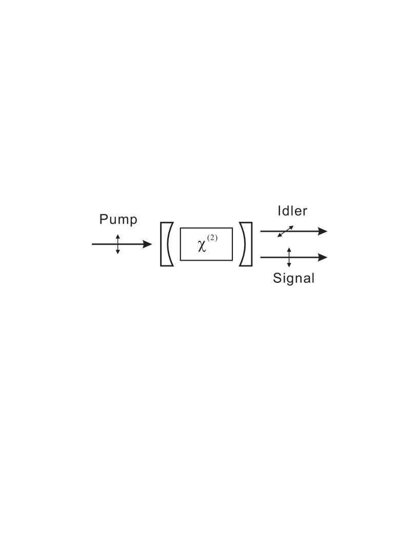
FIG. 1.: Schematic of a doubly-resonant optical parametric amplifier.

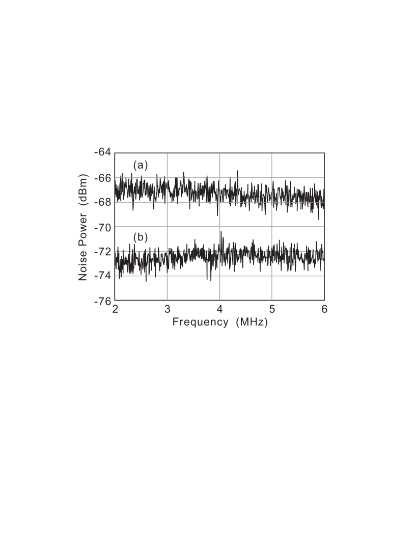
FIG. 2.: Shot-noise level (a), and signal-minus-idler intensity difference (b), from a KTP optical parametric oscillator.

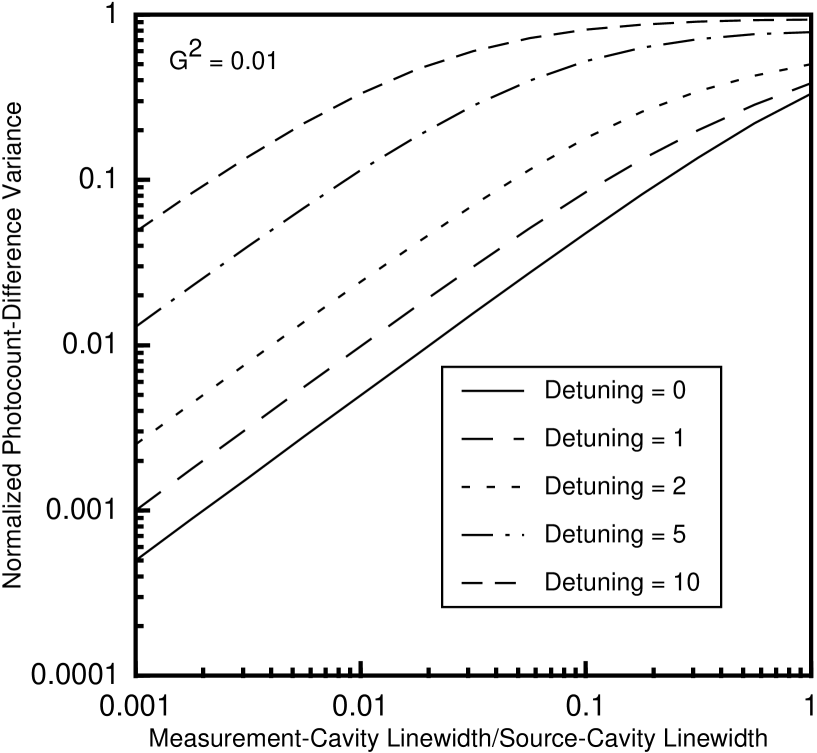
FIG. 3.: Normalized photocount-difference variance, $\sigma^{2}_{n}$, vs. the ratio of measurement-cavity linewidth to source-cavity linewidth, $\Gamma_{c}/\Gamma$, for 1% OPA pumping ($G^{2}=0.01$) and various values of the normalized detuning, $\Delta\omega/\Gamma$.

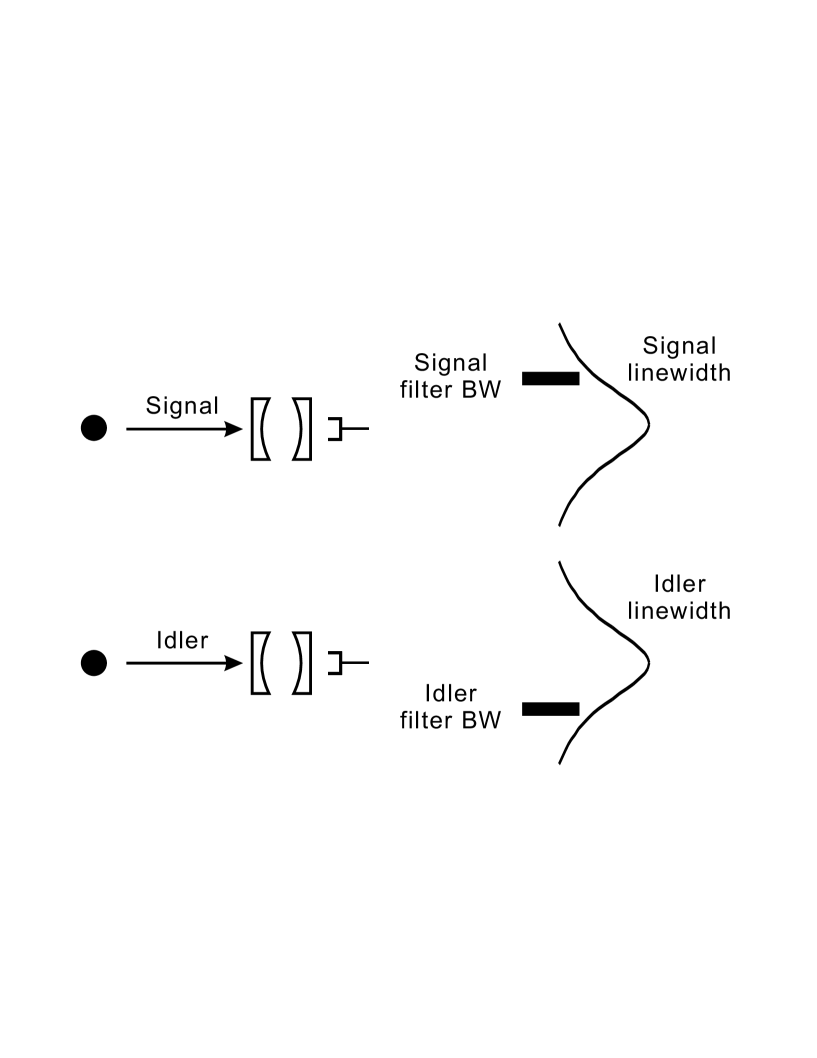
FIG. 4.: Schematic for filter-penetration optical magic bullets. BW: bandwidth.

- [1] C. H. Bennett and P. W. Shor, IEEE Trans. Inform. Theory IT-44, 2724 (1998).
- [2] A. Einstein, B. Podolsky, and N. Rosen, Phys. Rev. 47, 777 (1935).
- [3] A. Furusawa, J. L. Sørensen, S. L. Braunstein, C. A. Fuchs, H. J. Kimble, and E. S. Polzik, Science 282, 706 (1998).
- [4] S. L. Braunstein, Phys. Rev. Lett. 80, 4084 (1998).
- [5] S. L. Braunstein, Nature 394, 47 (1998).
- [6] S. Lloyd and J.-J. E. Slotine, Phys. Rev. Lett. 80, 4088 (1998).
- [7] S. Lloyd and S. L. Braunstein, Phys. Rev. Lett. 82, 1784 (1999).
- [8] J. H. Shapiro and K.-X. Sun, J. Opt. Soc. Am. B 11, 1130 (1994).
- [9] J. H. Shapiro and N. C. Wong, J. Opt. B: Quantum Semiclass. Opt. 2, L1 (2000).
- [10] H. P. Yuen and J. H. Shapiro, IEEE Trans. Inform. Theory IT-26, 78 (1980).
- [11] S. Reynaud, C. Fabre, and E. Giacobino, J. Opt. Soc. Am. B 4, 1520 (1987).
- [12] K. W. Leong, N. C. Wong, and J. H. Shapiro, Opt. Lett. 15, 1058 (1990).
- [13] J. Teja and N. C. Wong, Opt. Express 2, 65 (1998).
- [14] J. H. Shapiro, “Long-distance high-fidelity teleportation using singlet states,” to appear in Proc. Fifth International Conf. on Quantum Communication, Measurement, and Computing, Capri, 2000, edited by O. Hirota and P. Tombesi.
- [15] L.-A. Wu, H. J. Kimble, J. L. Hall, and H. Wu, Phys. Rev. Lett. 57, 2520 (1986).
- [16] M. Vasilyev, S. K. Choi, P. Kumar, and G. M. D’Ariano, Phys. Rev. Lett. 84, 2354 (2000).
- [17] S. Lloyd, M. S. Shahriar, and P. R. Hemmer, “Teleportation and the quantum Internet,” submitted to Phys. Rev. A. (quant-ph/003147)