Coherent Phenomena in Photonic Crystals

Abstract

We study the spontaneous emission, the absorption and dispersion properties of a ${\bf\Lambda}$-type atom where one transition interacts near resonantly with a double-band photonic crystal. Assuming an isotropic dispersion relation near the band edges, we show that two distinct coherent phenomena can occur. First, the spontaneous emission spectrum of the adjacent free space transition obtains ‘dark lines’ (zeroes in the spectrum). Second, the atom can become transparent to a probe laser field coupling to the adjacent free space transition.

I Introduction

It has been well established over the years that spontaneous emission depends not only on the properties of the excited atomic system but also on nature of the surrounding environment and more specifically on the density of electromagnetic vacuum modes. Purcell [1] was the first to predict that the rate of spontaneous emission for atomic transitions resonant with cavity frequencies could be enhanced due to the strong frequency dependence of the density of modes. Employing a similar idea, Kleppner [2] showed that spontaneous emission in a waveguide may be suppressed below the free space level due to the singular behaviour of the density of modes near the fundamental threshold frequency of the waveguide.

The above studies attracted recent attention when it was realized that periodic dielectric structures could be engineered in such way that gaps in the allowed photon frequencies may appear [3]. Since then, photonic band gap (PBG) materials exhibiting photon localization have been fabricated initially at microwave frequencies and more recently at near infrared and optical frequencies. The study of quantum and nonlinear optical phenomena in atoms (impurities) embedded in such structures, lead to the prediction of many interesting effects [3]. As examples we mention the localization of light and the formation of single-photon [4, 5, 6, 7] and two-photon [8] ‘photon-atom bound states’, suppression and even complete cancellation of spontaneous emission [9, 10, 11, 12], population trapping in two-atom systems [12], phase dependent behaviour of the population dynamics [13, 14], enhancement of spontaneous emission interference [15, 16, 17], modified reservoir induced transparency [18, 19, 20] and transient lasing without inversion [21], occurrence of dark lines in spontaneous emission [22, 23] and other phenomena [24, 25, 26]. In addition there is also current interest with regard to the feasibility of the observation of either the quantum Zeno effect [27] or the quantum Anti-Zeno effect [28] in modified reservoirs, such as the PBG.

In this paper we study the spontaneous emission and the probe absorption/dispersion spectrum in a ${\bf\Lambda}$-type system, similar to the one used in previous studies [10, 13, 18, 21, 22, 24, 29], with one of the atomic transitions decaying spontaneously in a double-band [17] PBG reservoir. We show that the spontaneous emission spectrum can exhibit ‘dark lines’ (zeroes in the spectrum at certain values of the emitted photon frequency) in the spontaneous emission spectrum in the free space transition. In addition, the atom becomes transparent to a probe laser field coupling to the free space transition, which exhibits ultra-slow group velocities near the transparency window. The dependence of these phenomena on the width of the gap is examined and a comparison with the single-band case results is made [18, Paspalakisb].

This article is organized as follows. In section II we apply the time-dependent Schrödinger equation to describe the interaction of our system with the modified vacuum, calculate the spontaneous emission spectrum in the free space reservoir and discuss its properties along with the differences from the single-band case [10, 11]. In section III using the time-dependent Schrödinger equation we calculate analytically the steady state linear susceptibility of the system. Results of the absorption and dispersion of a probe laser field in this system and their comparison with the single-band case are also presented in section III. Finally, we summarize our findings in section IV.

II Equations and results for the spontaneous emission spectrum

We begin with the study of the $\Lambda$-type scheme, shown in Fig. 1(a). This system is similar to that used in previous studies [10, 13, 18, 21, 22, 24, 29]. The atom is assumed to be initially in state $|2\rangle$. The transition $|2\rangle\leftrightarrow|1\rangle$ is taken to be near resonant with a modified reservoir (this will be later referred to as the non-Markovian reservoir), while the transition $|2\rangle\leftrightarrow|0\rangle$ is assumed to be occurring in free space (this will be later referred to as the Markovian reservoir). The spectrum of this latter transition is of central interest in this section. The Hamiltonian which describes the dynamics of this system, in the interaction picture and the rotating wave approximation (RWA), is given by (we use units such that $\hbar=1$),

$$H = \sum_{{\bf\lambda}}g_{{\bf\lambda}}e^{-i(\omega_{\bf\lambda}-\omega_{20})t}|2\rangle\langle 0|a_{{\bf\lambda}}+\sum_{{\bf\kappa}}g_{{\bf\kappa}}e^{-i(\omega_{\bf\kappa}-\omega_{21})t}|2\rangle\langle 1|a_{{\bf\kappa}}+\mbox{H.c.}\,.$$ (1)

Here, $g_{{\bf\kappa}}$ denotes the coupling of the atom with the modified vacuum modes $({\bf\kappa})$ and $g_{{\bf\lambda}}$ denotes the coupling of the atom with the free space vacuum modes $({\bf\lambda})$. Both coupling strengths are taken to be real. The energy separations of the states are denoted by $\omega_{ij}=\omega_{i}-\omega_{j}$ and $\omega_{\bf\kappa}$ $(\omega_{\bf\lambda})$ is the energy of the ${\bf\kappa}$ $({\bf\lambda})$-th reservoir mode.

The description of the system is done via a probability amplitude approach. We proceed by expanding the wave function of the system, at a specific time $t$, in terms of the ‘bare’ state vectors such that

$$|\psi(t)\rangle=b_{2}(t)|2,\{0\}\rangle+\sum_{{\bf\lambda}}b_{{\bf\lambda}}(t)|0,\{{\bf\lambda}\}\rangle+\sum_{{\bf\kappa}}b_{{\bf\kappa}}(t)|1,\{{\bf\kappa}\}\rangle\,.$$ (2)

Substituting Eqs. (1) and (2) into the time-dependent Schrödinger equation we obtain

$$i\dot{b}_{2}(t) = \sum_{\bf\lambda}g_{{\bf\lambda}}b_{\bf\lambda}(t)e^{-i(\omega_{{\bf\lambda}}-\omega_{20})t}+\sum_{\bf\kappa}g_{{\bf\kappa}}b_{\bf\kappa}(t)e^{-i(\omega_{{\bf\kappa}}-\omega_{21})t}\,,$$ (3)

$$i\dot{b}_{\bf\lambda}(t) = g_{{\bf\lambda}}b_{2}(t)e^{i(\omega_{{\bf\lambda}}-\omega_{20})t}\,,$$ (4)

$$i\dot{b}_{\bf\kappa}(t) = g_{{\bf\kappa}}b_{2}(t)e^{i(\omega_{{\bf\kappa}}-\omega_{21})t}\,.$$ (5)

We proceed by performing a formal time integration of Eqs. (4) and (5) and substitute the result into Eq. (3) to obtain the integro-differential equation

$$\dot{b}_{2}(t) = -\int^{t}_{0}dt^{\prime}b_{2}(t^{\prime})\sum_{\bf\lambda}g^{2}_{{\bf\lambda}}e^{-i(\omega_{{\bf\lambda}}-\omega_{20})(t-t^{\prime})}-\int^{t}_{0}dt^{\prime}b_{2}(t^{\prime})\sum_{\bf\kappa}g^{2}_{{\bf\kappa}}e^{-i(\omega_{{\bf\kappa}}-\omega_{21})(t-t^{\prime})}\,.$$ (6)

Because the reservoir with modes $\lambda$ is assumed to be Markovian, we can apply the usual Weisskopf-Wigner result [3] and obtain

$$\sum_{\bf\lambda}g^{2}_{{\bf\lambda}}e^{-i(\omega_{{\bf\lambda}}-\omega_{20})(t-t^{\prime})}=\frac{\gamma}{2}\delta(t-t^{\prime})\,.$$ (7)

Note that the principal value term associated with the Lamb shift which should accompany the decay rate term has been omitted in Eq. (7). This does not affect our results, as we can assume that the Lamb shift is incorporated into the definition of our state energies. For the second summation in Eq. (6), the one associated with the modified reservoir modes, the above result is not applicable as the density of modes of this reservoir is assumed to vary much quicker than that of free space. To tackle this problem, we define the following kernel

$$K(t-t^{\prime})=\sum_{{\bf\kappa}}g^{2}_{{\bf\kappa}}e^{-i(\omega_{\bf\kappa}-\omega_{21})(t-t^{\prime})}\approx\beta^{3/2}\int d\omega\rho(\omega)e^{-i(\omega-\omega_{21})(t-t^{\prime})}\,,$$ (8)

with $\beta$ being the atom-modified reservoir resonant coupling constant. The above kernel is calculated using the appropriate density of modes $\rho(\omega)$ of the modified reservoir. Using Eqs. (7) and (8) into Eq. (6) we obtain

$$\dot{b}_{2}(t) = -\frac{\gamma}{2}b_{2}(t)-\int^{t}_{0}dt^{\prime}b_{2}(t^{\prime})K(t-t^{\prime})\,.$$ (9)

The long time spontaneous emission spectrum in the Markovian reservoir is given by $S(\delta_{\bf\lambda})\propto|b_{\bf\lambda}(t\rightarrow\infty)|^{2}$, with $\delta_{\bf\lambda}=\omega_{\bf\lambda}-\omega_{20}$. We calculate $b_{\bf\lambda}(t\rightarrow\infty)$ with the use of the Laplace transform of the equations of motion. Using Eq. (4) and the final value theorem we obtain the spontaneous emission spectrum as $S(\delta_{{\bf\lambda}})\propto{\gamma}|\lim_{s\rightarrow-i\delta_{{\bf\lambda}}}B_{2}(s)|^{2}$, where $B_{2}(s)=\int^{\infty}_{0}dte^{-st}b_{2}(t)$ is the Laplace transform of the atomic amplitudes $b_{2}(t)$ and $s$ is the Laplace variable. This in turn, with the help of Eq. (9), reduces to

$$S(\delta_{{\bf\lambda}})\propto\frac{\gamma}{\left|-i\delta_{\bf\lambda}+\gamma/2+\tilde{K}(s\rightarrow-i\delta_{\bf\lambda})\right|^{2}}\,.$$ (10)

Here, $\tilde{K}(s)=\int^{\infty}_{0}dte^{-st}K(t)$ is the Laplace transform of $K(t)$, which yields from Eq. (8),

$$\tilde{K}(s)=\beta^{3/2}\int d\omega\frac{\rho(\omega)}{s+i(\omega-\omega_{21})}\,.$$ (11)

Therefore, in order to calculate the spontaneous emission spectrum in the Markovian reservoir we need to calculate $\tilde{K}(s)$.

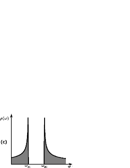
We consider the case of a double-band isotropic model of the photonic crystal, which has an upper band, a lower band and a forbidden gap, the near the edges dispersion relation [17] is approximated by

$$\omega_{\kappa}=\omega_{g1}-A_{1}(\kappa-\kappa_{0})^{2}\ \,\kappa<\kappa_{0}$$ , (12)

$$\omega_{\kappa}=\omega_{g2}+A_{2}(\kappa-\kappa_{0})^{2}\ \,\kappa>\kappa_{0}\,,$$ , (13)

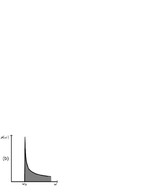
with $A_{n}\approx\omega_{gn}/{\kappa}_{0}^{2}$, $(n=1,2)$. Then the density of modes reads,

$$\rho(\omega)=\frac{1}{2\pi}\left[\frac{1}{\sqrt{\omega_{g1}-\omega}}\Theta(\omega_{g1}-\omega)+\frac{1}{\sqrt{\omega-\omega_{g2}}}\Theta(\omega-\omega_{g2})\right]\,,$$ (14)

where $\omega_{gn}$ is the gap frequency and $\Theta$ is the Heaviside step function (as shown in Fig. 1(c)). Then, from Eq. (11) we obtain

$$\tilde{K}(s)=\frac{1}{2}\left(\frac{\beta^{3/2}\sqrt{i}}{\sqrt{s+i\delta_{g1}}}+\frac{\beta^{3/2}}{\sqrt{i}\sqrt{s+i\delta_{g2}}}\right)\,,$$ (15)

with $\delta_{gn}=\omega_{gn}-\omega_{21}$.

We use the formulae obtained above and calculate the spontaneous emission for several parameters of the system. From Eqs. (10) and (15) is obvious that the spectrum exhibits two zeros (i.e. predicts the existence of two dark lines), at $\delta_{\lambda}=\delta_{g1}$ and $\delta_{\lambda}=\delta_{g2}$. This is purely an effect of the density of modes of Eq. (15), and the non-Markovian character of the reservoir. In the case of a Markovian reservoir the spontaneous emission spectrum would obtain the well-known Lorentzian profile and no dark line would appear in the spectrum. The behaviour of the spectrum is shown in Fig. 2. In Fig. 2(a) we show an asymmetric case where the right hand side (rhs) threshold detuning $(\delta_{g2})$ is kept constant while the left hand side (lhs) threshold detuning $(\delta_{g1})$ is changed. There are three peaks and two zeroes in the spectrum, one pronounced peak in the center and two lower peaks in the sides. As $\delta_{g1}$ goes further to the sides the lhs peak is suppressed and the spectrum approximates that of the single band case[10, 11] which is shown in Fig. 3. That is because the lhs singularity in the density of the reservoir modes, Fig 1.  is far detuned from the atomic transition.

In Fig. 2(b) we show a symmetric spectrum, which is the case when the atom is placed in the middle of the gap. This spectrum also has two zeroes and three peaks. In this case when the threshold detunings increase (i.e, the width of the gap increases) the spectrum approximates the Lorentzian shape. This is a result of the complete cancelation of any emission in the modified reservoir as there are no modes available for a large range of frequencies around the relevant atomic transition.

III Equations and results for the probe absorption/dispersion spectrum

The aim in this section is to investigate the absorption and dispersion properties of our system for a weak probe laser field. As the probe laser field is assumed to be weak the probability amplitude approach can be employed for the description of the system. The Hamiltonian of the system, in the interaction picture and the rotating wave approximation, is given by,

$$H = \Omega e^{i\delta t}|0\rangle\langle 2|+\sum_{{\bf\lambda}}g_{{\bf\lambda}}e^{-i(\omega_{\bf\lambda}-\omega_{20})t}|2\rangle\langle 0|a_{{\bf\lambda}}+\sum_{{\bf\kappa}}g_{{\bf\kappa}}e^{-i(\omega_{\bf\kappa}-\omega_{21})t}|2\rangle\langle 1|a_{{\bf\kappa}}+\mbox{H.c.}\,.$$ (16)

Here, $\Omega$ is the Rabi frequency (assumed real for simplicity) and $\delta=\omega-\omega_{20}$ is the laser detuning from resonance with the $|0\rangle\leftrightarrow|2\rangle$ transition with $\omega$ being the angular frequency of the probe laser field. We note that we are interested in the perturbative behaviour of the system to the probe laser pulse, therefore we can eliminate the Markovian decay modes using the method presented in the previous section and study the system using the following effective Hamiltonian

$$H=\bigg{[}\Omega e^{i\delta t}|0\rangle\langle 2|+\sum_{\kappa}g_{\kappa}e^{-i(\omega_{\kappa}-\omega_{21})t}|2\rangle\langle 1|a_{\kappa}+\mbox{H.c.}\bigg{]}-i\frac{\gamma}{2}|2\rangle\langle 2|\,.$$ (17)

The wavefunction of the system, at a specific time $t$, can be expanded in terms of the ‘bare’ eigenvectors such that

$$|\psi(t)\rangle=c_{0}(t)|0,\{0\}\rangle+c_{2}(t)e^{-i\delta t}|2,\{0\}\rangle+\sum_{{\bf\kappa}}c_{{\bf\kappa}}(t)|1,\{{\bf\kappa}\}\rangle\,,$$ (18)

and $c_{0}(t=0)=1$, $c_{2}(t=0)=0$, $c_{\kappa}(t=0)=0$. Substituting Eqs. (17) and (18) into the time-dependent Schrödinger equation and eliminating the vacuum amplitude $c_{\kappa}(t)$, we obtain the time evolution of the probability amplitudes as

$$i\dot{c}_{0}(t) = \Omega c_{2}(t)\,,$$ (19)

$$i\dot{c}_{2}(t) = \Omega c_{0}(t)-\left(\delta+i\frac{\gamma}{2}\right)c_{2}(t)-i\int^{t}_{0}dt^{\prime}K^{\prime}(t-t^{\prime})c_{2}(t^{\prime})\,,$$ (20)

with the kernel

$$K^{\prime}(t-t^{\prime}) = \sum_{\kappa}g^{2}_{\kappa}e^{-i(\omega_{\kappa}-\omega_{21}-\delta)(t-t^{\prime})}\approx K(t)e^{i\delta t}\,.$$ (21)

All the coupling constants ($g_{\kappa}$, $\beta$, $\Omega$) are assumed to be real, for simplicity.

The equation of motion for the electric field amplitude $E(z,t)$ is given by [Harris92a],

$$\left(\frac{\partial}{\partial z}+\frac{1}{v_{g}}\frac{\partial}{\partial t}\right)E(z,t)=-i\frac{\omega}{2c}\chi(\delta)E(z,t)\,,$$ (22)

where $\chi(\delta)$ is the linear susceptibility of the medium and $v_{g}=c/[1+(\omega/2)(\partial\mbox{Re}(\chi)/\partial\omega)]$ is the group velocity of the laser pulse with the derivative of the real part of the susceptibility being evaluated at the carrier frequency.

Since the transition $|0\rangle\leftrightarrow|2\rangle$ is treated as occurring in free space, the steady state linear susceptibility is given by

$$\chi(\delta)=-\frac{4\pi{\cal N}|\mbox{\boldmath${\mu}$\unboldmath${}_{02}$}|^{2}}{\Omega(z,t)}c_{0}(t\rightarrow\infty)c^{*}_{2}(t\rightarrow\infty)\,,$$ (23)

with ${\cal N}$ being the atomic density.

Therefore, in order to determine the steady state absorption properties we have to solve Eqs. (19), (20) for long times. We assume that the laser-atom interaction is very weak $(\Omega\ll\beta,\gamma)$ so that $c_{0}(t)\approx 1$ for all times, and by using perturbation theory, Eqs. (19) and (20) reduce to

$$i\dot{c}_{2}(t) \approx \Omega-\left(\delta+i\frac{\gamma}{2}\right)c_{2}(t)-i\int^{t}_{0}dt^{\prime}K^{\prime}(t-t^{\prime})c_{2}(t^{\prime})\,.$$ (24)

We further assume that $\Omega(z,t)$ is approximately constant in the medium and with the use of the Laplace transform we obtain from Eq. (24)

$${C}_{2}(s)=\frac{\Omega}{s\left[\delta+i\gamma/2+i\tilde{K}(s)+is\right]}\,.$$ (25)

If $\gamma\neq 0$ then the terms inside the brackets of Eq. (25) have only complex, not purely imaginary, roots. Therefore we can easily obtain, using the final value theorem, the long time behaviour of the probability amplitude,

$$c_{2}(t\rightarrow\infty) = \lim_{s\rightarrow 0}[C_{2}(s)]$$ (26)

$$= \frac{\Omega}{\delta+i\gamma/2+i\tilde{K^{\prime}}(s\rightarrow 0)}$$ (27)

$$= \frac{\Omega}{\delta+i\gamma/2+i\tilde{K}(-i\delta)}\,.$$ (28)

Using Eqs. (23) and (28) we find that the steady state linear susceptibility of our system is given by

$$\chi(\delta)=-\frac{4\pi{\cal N}|\mbox{\boldmath${\mu}$\unboldmath${}_{02}$}|^{2}}{\delta-i\gamma/2-i\tilde{K^{*}}(-i\delta)}\,.$$ (29)

Therefore, the absorption and dispersion of the probe laser field are determined by the density of modes of the non-Markovian reservoir. In our case the linear susceptibility becomes zero at $\delta=\delta_{g1}$ and $\delta=\delta_{g2}$, therefore the medium becomes transparent to the laser field. This result is in contrast with the case in which the transition $|2\rangle\leftrightarrow|1\rangle$ occurs in free space, where the well-known Lorentzian absorption profile is obtained. Typical spectra are shown in Fig. 4, where only the lhs threshold detuning is changed. Both the absorption and dispersion spectra are asymmetric and their shape depends critically on the detunings. We note that Fig. 4(c) resembles as expected, the corresponding spectra in the case of a single band reservoir [18] which is shown in Fig. 5.

We also present the case of symmetric spectra in Fig. 6, where the detunings are symmetrically changed i.e., with the transition frequency of the atom in the middle of the gap. Here the interesting effect is best shown in Figs. 6(a) and 6(b) where the transparency effect in the sides of the spectra is combined with the usual absorption/dispersion profile near the center of the spectrum.

We note that besides the transparency effect which occurs for the predicted values of frequency, we note that the group velocity of the probe laser pulse is also effectively reduced near the transparency window due to the steepness of the dispersion curve. These results are related to that of electromagnetically induced transparency (EIT) in a four-level laser-driven tripod scheme [30]. However, EIT occurs through the application of external laser fields. Here, transparency is intrinsic to the system as it occurs due to the presence of a square root singularity of the density of modes at the band edges.

IV Summary

In this article we studied the spontaneous emission, absorption and dispersion spectra of a three-level atom embedded in a two-band isotropic photonic crystal. For the spontaneous emission we have shown that the spectrum exhibits two dark lines and can be significantly modified via the system parameters. The explicit dependance of the spectrum on the width of the gap and on various values of the atomic parameters was also analyzed. For the absorption and dispersion spectra, two transparency windows exist. Near the transparency windows a very slow group velocity for the laser pulse is obtained. In this case too, the spectra depend critically on the atomic parameters and the width of the gap.

FIG. 1.: Figure (a) displays a three level, ${\bf\Lambda}$-type atomic system. The thick dashed line denotes the coupling to the modified reservoir (PBG) and the thin dashed line denotes the background decay. Figure (b) shows the density of modes for the case of the single-band isotropic PBG model. Figure (c) shows the density of modes for the case of the double-band isotropic PBG model.

FIG. 2.: The spontaneous emission spectrum $S(\delta_{\bf\lambda})$ (in arbitrary units) for the double-band case and parameters $\gamma=1$ and (a) ($\delta_{g1}=-1$, $\delta_{g2}=0$) (full curve), ($\delta_{g1}=-2$, $\delta_{g2}=0$) (dashed curve), ($\delta_{g1}=-3$, $\delta_{g2}=0$) (dot-dashed curve), (b) ($\delta_{g1}=-1$, $\delta_{g2}=1$) (full curve), ($\delta_{g1}=-2$, $\delta_{g2}=2$) (dashed curve), ($\delta_{g1}=-3$, $\delta_{g2}=3$) (dot-dashed curve).

FIG. 3.: The spontaneous emission spectrum $S(\delta_{\bf\lambda})$ (in arbitrary units) for the single-band case and parameters $\gamma=1$ and $\delta_{g}=0$ (full curve); $\delta_{g}=1$ (dashed curve); $\delta_{g}=-1$ (dot-dashed curve). All parameters are in units of $\beta$.

FIG. 4.: The absorption and dispersion spectra (in arbitrary units) for the double-band case for parameters (a) ($\delta_{g1}=-1$, $\delta_{g2}=0$), (b) ($\delta_{g1}=-2$, $\delta_{g2}=0$), (c) ($\delta_{g1}=-3$, $\delta_{g2}=0$).

FIG. 5.: The absorption and dispersion spectra (in arbitrary units) for the single-band case for parameters $\gamma=1$, $\delta_{g}=0$. The solid curve is the absorption profile ($-$Im$[\chi(\delta)]$) while the dashed curve the dispersion profile (Re$[\chi(\delta)]$).

FIG. 6.: The absorption and dispersion spectra (in arbitrary units) for the double-band case for parameters (a) ($\delta_{g1}=-1$, $\delta_{g2}=1$), (b) ($\delta_{g1}=-2$, $\delta_{g2}=2$), (c) ($\delta_{g1}=-3$, $\delta_{g2}=3$).

REFERENCES

- [1] E.M. Purcell, Phys. Rev. 69, 681 (1946).
- [2] D. Kleppner, Phys. Rev. Lett. 47, 233 (1981).
- [3] For a recent review in the subject see, P. Lambropoulos, G.M. Nikolopoulos, T.R. Nielsen and S. Bay, Rep. Prog. Phys. 63, 455 (2000).
- [4] S. John, Phys. Rev. Lett. 58, 2486 (1987).
- [5] S. John and J. Wang, Phys. Rev. Lett. 64, 2418 (1990); Phys. Rev. B 43, 12772 (1990).
- [6] S. John and T. Quang, Phys. Rev. Lett. 74, 3419 (1995).
- [7] S.-Y. Zhu, Y.P. Yang, H. Chen, H. Zheng and M.S. Zubairy, Phys. Rev. Lett. 84, 2136 (2000).
- [8] G.M. Nikolopoulos and P. Lambropoulos, Phys. Rev. A 61, 053812 (2000)
- [9] E. Yablonovitch, Phys. Rev. Lett. 58, 2059 (1987).
- [10] S. John and T. Quang, Phys. Rev. A 50, 1764 (1994).
- [11] A.G. Kofman, G. Kurizki and B. Sherman, J. Mod. Opt. 41, 353 (1994).
- [12] S. Bay, P. Lambropoulos and K. Mølmer, Phys. Rev. A 55, 1485 (1997).
- [13] T. Quang, M. Woldeyohannes, S. John and G.S. Agarwal, Phys. Rev. Lett. 79, 5238 (1997).
- [14] M. Woldeyhannes and S. John, Phys. Rev. A 60, 5046 (1999).
- [15] S.-Y. Zhu, H. Chen and H. Huang, Phys. Rev. Lett. 79, 205 (1997).
- [16] Y.P. Yang and S.-Y. Zhu, Phys. Rev. A 61, 043809 (2000).
- [17] Y.P. Yang and S.-Y. Zhu, J. Mod. Opt. 47, 1513 (2000).
- [18] E. Paspalakis, N.J. Kylstra and P.L. Knight, Phys. Rev. A 60, R33 (1999).
- [19] H. Lee, S.-Y. Zhu and M.O. Scully, Laser Phys. 9, 831 (1999).
- [20] M. Erhard and C.H. Keitel, Opt. Commun. 179, 517 (2000).
- [21] D.G. Angelakis, E. Paspalakis and P.L. Knight, Phys. Rev. A 61, 055802 (2000).
- [22] E. Paspalakis, D.G. Angelakis and P.L. Knight, Opt. Commun. 172, 229 (1999).
- [23] Y.P. Yang, Z.X. Lin, S.-Y. Zhu, H. Chen and W.G. Feng, Phys. Lett. A 270, 41 (2000).
- [24] S. Bay, P. Lambropoulos and K. Mølmer, Phys. Rev. Lett. 79, 2654 (1997).
- [25] N. Vats and S. John, Phys. Rev. A 58, 4168 (1998).
- [26] G.M. Nikolopoulos and P. Lambropoulos, Phys. Rev. A 60, 5079 (1999).
- [27] A.G. Kofman and G. Kurizki, Phys. Rev. A 54, R3750 (1996).
- [28] M. Lewenstein and K. Rza̧żewski, Phys. Rev. A 61, 02215 (2000).
- [29] M. Lewenstein, J. Zakrzewski, T.W. Mossberg and J. Mostowski, J. Phys. B 21, L9 (1988); M. Lewenstein, J. Zakrzewski and T.W. Mossberg, Phys. Rev. A 38, 808 (1988).
- [30] E. Paspalakis and P.L. Knight, submitted for publication (2000).