Information Tradeoff Relations for Finite-Strength Quantum Measurements LA-UR-00-4403

Abstract

In this paper we give a new way to quantify the folklore notion that quantum measurements bring a disturbance to the system being measured. We consider two observers who initially assign identical mixed-state density operators to a two-state quantum system. The question we address is to what extent one observer can, by measurement, increase the purity of his density operator without affecting the purity of the other observer’s. If there were no restrictions on the first observer’s measurements, then he could carry this out trivially by measuring the initial density operator’s eigenbasis. If, however, the allowed measurements are those of finite strength—i.e., those measurements strictly within the interior of the convex set of all measurements—then the issue becomes significantly more complex. We find that for a large class of such measurements the first observer’s purity increases the most precisely when there is some loss of purity for the second observer. More generally the tradeoff between the two purities, when it exists, forms a monotonic relation. This tradeoff has potential application to quantum state control and feedback.

03.67.-a,02.50.-r,03.65.Bz

]

I Introduction

Since the earliest days of quantum mechanics, a common idea associated with the measurement process has been that it necessarily disturbs or interferes with the system being observed. For instance Bohr, in his reply to the Einstein-Podolsky-Rosen paper [1], writes that the quantum description “may be characterized as a rational utilization of all possibilities of unambiguous interpretation … compatible with the finite and uncontrollable interaction between the objects and the measuring instruments” [2, 3]. Or Pauli, on a much later occasion, writes again, “every act of observation is an interference, of undeterminable extent, with the instruments of observation as well as with the system observed, and interrupts the causal connection between the phenomena preceding and succeeding it” [6]. See Refs. [7, 8] for a more complete bibliographic account of this issue.

Without question, it has also been apparent since the earliest days of the theory that these proclamations are somewhat dubious. The question is this: What is it that is being interfered with or disturbed in a measurement? If there were a set of hidden variables underneath the statistical predictions of quantum theory, then the answer would be at hand: The act of measurement disturbs the hidden variables. In the absence of a hidden-variable explanation [9], however, this becomes a moot point. Measuring x cannot disturb p if p does not have an independent existence before a measurement elicits its value [10]. In fact one has to wonder why the word “measurement” is used at all in this context: If there are no free-standing values x and p to disturb, then surely there are no values to measure either.

Eschewing metaphysical concerns, one might try to give a precise sense to the idea that measurements cause disturbance by focusing solely on the wavefunction itself. For, the wavefunction appears to be the simplest term in the theory that would even allow a precise formulation of the question. One might say for instance, “The word measurement is a misnomer for our experimental interventions into the course of nature [11, 12]. The unpredictable wavefunction collapse is the quantitative signature of a disturbance in quantum measurement. Since the state change is random, the measurement causes an uncontrollable disturbance.” But this formulation too is not without problem. The quantum state resulting from a measurement depends in a crucial way on the precise form of the measurement interaction [13]. In particular, if there is only a single quantum state under scrutiny—as was the case in the original Heisenberg uncertainty relation discussion [14]—or even an unknown state drawn from a fixed orthogonal set [15], then a measurement interaction can always be rigged for any observable so that, upon completion of the process, the quantum state is returned to its initial value [16]. It does not matter that the measurement outcome is random and unpredictable: If the discussion is limited to a single quantum state or an orthogonal set, then there need be no disturbance in the sense of a necessary wavefunction change.

What appears to be needed is a situation where more than one quantum state from within a nonorthogonal set arises naturally into the considerations. Indeed, perhaps the first phenomenon to give a precise meaning to the idea that information-gathering measurements necessarily cause an accompanying disturbance is quantum cryptography [17, 18]. There it is essential that the systems are known to be prepared in one or another quantum state drawn from some fixed nonorthogonal set [19, 20, 21]. These nonorthogonal states are used to encode a potentially secret cryptographic key to be shared between the sender and receiver. In this case, the information an eavesdropper seeks is not about some nonexistent hidden variable like $x$ or $p$, but instead about which quantum state was actually prepared in each individual transmission. What is novel here is that the encoding of the proposed key into nonorthogonal states forces the information-gathering process to induce a disturbance to the overall set of states. That is, the presence of an active eavesdropper transforms the initial pure states into a set of mixed states or, at the very least, into a set of pure states with larger overlaps than before. This action ultimately boils down to a loss of predictability for the sender over the outcomes of the receiver’s measurements and, so, is directly detectable by the receiver revealing some of those outcomes for the sender’s inspection. In fact, there is a direct connection between the statistical information gained by an eavesdropper and the consequent disturbance she must induce to the quantum states in the process. As the information gathered goes up, the necessary disturbance also goes up in a precisely formalizable way [22, 23, 24].

Note the two ingredients that appear in this formulation. First, the information gathering or measurement is grounded with respect to one observer (in this case, the eavesdropper), while the disturbance is grounded with respect to another (here, the sender). In particular, the disturbance is a disturbance to the sender’s previous information—this is measured by his diminished ability to predict the outcomes of certain measurements the legitimate receiver might perform. No hint of any variable intrinsic to the system is made use of in this formulation. In itself, this is already a rupture from the founding fathers’ description of disturbance in measurement. As far as we can tell, all early literature on the subject refers the discussion of disturbance exclusively to the system and the invasive measuring device, not to the perspective of various observers [7].

The second ingredient is another break with the founding fathers. One must consider at least two possible nonorthogonal preparations in order for the formulation to have any meaning. This is because the information gathering is not about some classically-defined observable—i.e., about some unknown hidden variable or reality intrinsic to the system—but is instead about which of the unknown states the sender actually prepared. The lesson is this: Forget about the unknown preparation, and the random outcome of the quantum measurement is information about nothing. It is simply “quantum noise” with no connection to any preexisting variable.

How crucial is this second ingredient, i.e., that there be at least two nonorthogonal states within the set under consideration? We can start to readdress its necessity by making a slight shift in the account above. Divorcing the discussion from a cryptographic protocol, one might say that the eavesdropper’s goal is not so much to uncover the identity of the unknown quantum state, but to sharpen her predictability over the receiver’s measurement outcomes. In fact, she would like to do this at the same time as disturbing the sender’s predictions as little as possible. Changing the language still further to the terminology of Ref. [12], the eavesdropper’s actions serve to sharpen her information about the potential consequences of the receiver’s further interventions upon the system. (Again, she would like to do this while minimally diminishing the sender’s previous information about those same consequences.) In the cryptographic context, a byproduct of this effort is that the eavesdropper ultimately comes to a more sound prediction of the secret key. From the present point of view, however, the importance of this change of language is that it leads to an almost Bayesian perspective on the information–disturbance problem [25].

Within Bayesian probability theory, one of the overarching themes is to identify the conditions under which a set of decision-making agents can come to a common belief or probability assignment for some specified random variable even though the agents’ initial beliefs may differ [26]. One might similarly view the process of quantum eavesdropping. The sender and the eavesdropper start off initially with differing quantum state assignments for a single physical system. In this case it so happens that the sender can make sharper predictions than the eavesdropper about the outcomes of the receiver’s measurements. The eavesdropper, not satisfied with the situation, performs a measurement on the system in an attempt to sharpen those predictions. In particular, there is an attempt to come into something of an agreement with the sender but without revealing the outcomes of her measurements or, indeed, her very presence.

It is at this point that a distinct property of the quantum world makes itself known. The eavesdropper’s attempt to surreptitiously come into alignment with the sender’s predictability is always shunted away from its goal. This shunting of various observer’s predictability (and perhaps only this shunting [27]) is the subtle manner in which the quantum world is sensitive to our experimental interventions.

This motivates finally the following problem, which is the subject of our paper. Suppose two players—let us call them Alice and Bob from here out—come to agree about the way a quantum system will react to any measurement. In other words, by Gleason’s theorem [28], suppose they start with an identical density operator assignment $\rho$ for the system. The case we are interested in most is when $\rho$ is a mixed-state. Under what conditions can one player—Alice, say—surreptitiously increase her knowledge of the system without forcing the other player’s knowledge to become less relevant? (See Fig.1)

To move toward making this question precise, imagine that a third player will perform some measurement on the system in the future, but neither Alice nor Bob know which it will be. Depending upon which measurement is ultimately performed, Alice and Bob will have varying degrees of predictability for its outcomes. For instance, consider how their predictability fares with respect to various simple von Neumann measurements. If the measurement happens to be the eigenbasis of $\rho$, the Shannon entropy of the outcomes—which is a good measure of predictability [29]—will be the minimal value it can be [30]. This turns out to be the von Neumann entropy $S(\rho)=-{\rm tr}\,\rho\log\rho$. On the other hand, if the measurement happens to be a “mutually unbiased” basis [31] to the eigenbasis, then all measurement outcomes will be equally probable, and the outcome entropy will be $\log d$, where $d$ is the dimension of the system’s Hilbert space.

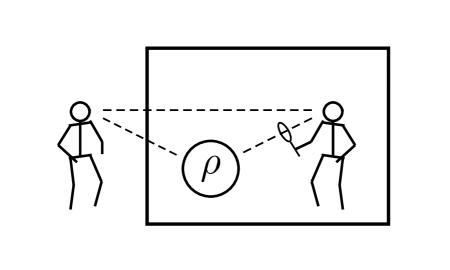
FIG. 1.: Here two observers both ascribe a density matrix $\rho$ to a quantum system. The observer inside the box (Alice) makes a measurement on the system without telling the result to the observer outside (Bob). Alice wishes to obtain as much knowledge about the final state of the system as she can, while causing as little disturbance to Bob’s state-of-knowledge as possible.

For the purpose at hand, we would like to capture in a single number something about how much Alice and Bob can predict of the unknown measurement. As a simple example, we might average the Shannon entropy of the measurement outcomes over the unique unitarily invariant measure (or “uniform” measure) on the space of von Neumann measurements [32, 33]. This would represent how well Alice and Bob will fare on average with respect to a completely random von Neumann measurement. Or, we might simply consider the entropy of the best case scenario, i.e., the von Neumann entropy of $\rho$ as above. Without getting specific—all will be made precise later—we will generically call measures of this flavor, measures of purity. The main intuition we want to capture is that when $\rho=|\psi\rangle\langle\psi|$ is a pure state, then Alice and Bob should generally have the most predictability over the third party’s measurements. When $\rho$ is the “completely mixed state”—i.e., proportional to the identity operator, $\rho=\frac{1}{d}I$—they should have the least.

The precise question we want to address is, can Alice secretly increase the purity of her quantum state assignment at the same time as leaving the other player’s purity unscathed? If she cannot, then such a failure may hint at another interesting way to quantify a quantum information–disturbance tradeoff. The hallmark of this formulation would be that it works even in the case where there is only a single initial quantum state (albeit a mixed state), while still capturing the shift in language we used to reformulate the quantum eavesdropping process.

Unfortunately, the answer is trivial if we leave the question posed in such a simplistic way. For, we need only suppose that Alice measures an eigenbasis $\Pi_{b}=|b\rangle\langle b|$ of $\rho$ to derail the whole program. Upon finding some result $b$, Alice will collapse her description of the system from the mixed state $\rho$ to the pure state [34]

$$\rho_{b}=\frac{1}{p_{b}}\Pi_{b}\rho\Pi_{b}\;,$$ (1)

where $p_{b}={\rm tr}(\rho\Pi_{b})$ is the probability of the particular outcome. The upshot of this is to make Alice’s final purity for the system maximal, while as far as Bob is concerned the system’s density operator will not be affected at all. This is because, with respect to Bob’s state of knowledge, the quantum state evolves simply to a mixture of Alice’s states, i.e.,

$$\rho\;\longrightarrow\;\sum_{b}p_{b}\rho_{b}=\rho\;,$$ (2)

and so his purity and indeed his quantum state assignment remain the same.

The key to finding something interesting here is to ask what would happen in the case where there is a well-justified restriction to the class of measurements Alice can perform. For instance, suppose Alice has not yet reached the technologically advanced stage of being able to perform a truly perfect von Neumann measurement. Maybe she is using a finite temperature Stern-Gerlach device to perform a spin measurement on an electron and, because of thermal noise, it every now and then registers a spin to be down when it should have registered a spin-up. To put this another way, instead of projecting $\rho$ into the states $\Pi_{0}$ and $\Pi_{1}$ as Alice would like, the Stern-Gerlach device projects $\rho$ according to a more general Lüder’s rule for positive operator valued measures (POVMs) [35, 36],

$$\rho\;\longrightarrow\;\rho_{b}=\frac{1}{p_{b}}E_{b}^{1/2}\rho E_{b}^{1/2}$$ (3)

where in this case

$$E_{0} = \kappa\Pi_{0}+(1-\kappa)\Pi_{1}\$$ (4)

$$E_{1} = (1-\kappa)\Pi_{0}+\kappa\Pi_{1}\;,$$ (5)

and $p_{b}={\rm tr}(\rho E_{b})$. Similarly, the description of the state change from Bob’s perspective must be in accord with this, and so is

$$\rho\;\longrightarrow\;\tilde{\rho}=\sum_{b}p_{b}\rho_{b}\;.$$ (6)

When $\kappa$ is a number strictly between 0 and 1, we will call this an instance of a finite-strength quantum measurement. (We use this suggestive terminology because we imagine that Alice can never really get to a perfect von Neumann measurement without the expenditure of an infinite amount of effort.) What can be said in a case like this?

Well, again, Alice will be able to generally increase the purity of her state without causing any decrease to Bob’s purity. She does this, as before, simply by choosing $\Pi_{0}$ and $\Pi_{1}$ to be eigenprojectors of $\rho$. Then $E_{0}$ and $E_{1}$ commute with the initial density operator, and it is straightforward to check that $\tilde{\rho}=\rho$. However, we can now ask whether this is the strategy that brings the greatest benefit to Alice. Might it be the case that Alice can increase her purity even more on average if she chooses $\Pi_{0}$ and $\Pi_{1}$ to be noncommuting with $\rho$? Moreover if it does, what kind of havoc will that wreak on Bob’s description of the system? What we are imagining here in the imagery of the Stern-Gerlach device is that though Alice may not be able to chill her magnets to absolute zero, she can at least adjust their spatial orientation at will. Is this a freedom she should make use of?

Interestingly, it turns out that there is a tradeoff in the two final purities. Whenever $\rho$ is nonpure (so that there is actually something to be “learned”) and $0<\kappa<1$ (so that the measurement is of finite strength), Alice’s final purity will be the greatest on average precisely when Bob’s purity has decreased the most in turn. Moreover, varying through the class of measurements that lead from the least average final purity to the most (with respect to Alice), we find that Bob’s purity goes down monotonically as Alice’s goes up. As we will show, this is an example of a more general phenomenon where the measurement operators are not so restricted as in Eqs. (4) and (5): for a large class of finite-strength quantum measurements, a nontrivial tradeoff relation always exists.

The plan of the remainder of the paper is as follows. In Section II, we give a precise formulation of the problem in the widest setting, including definitions of various measures of purity and also a definition of the general notion of a finite strength quantum measurement (without feedback). In Section III, we work out an analytic form for the changes of purity for both Alice and Bob under the assumption of a particularly simple measure of purity and the restriction that Alice’s quantum measurements have only two outcomes. We then explore the various regimes of the convex set of measurements and exhibit the general information tradeoff relation where it exists. We close in Section IV with a few concluding remarks about the significance of this result. In Appendix A, we prove that any efficient measurement (POVM) will increase Alice’s purity on average (for any measure of purity that is a convex function of the density operator’s eigenvalues)—this result is essentially identical to one proven recently in Ref. [37]. In Appendix B, for comparison with the main result here, we consider a variation of the problem where we vary over all measurements of a given finite strength instead of only those on the unitary orbits of a given fiducial measurement.

II Formulation

Our problem concerns two agents, Alice and Bob, who initially ascribe a single density operator $\rho$ to a quantum system in which they have some interest. The most important case for us is when $\rho$ is a mixed state, i.e., ${\rm tr}\rho^{2}<1$. For generality in the formulation, let us assume that $\rho$ is a density operator over a $d$-dimensional Hilbert space ${\cal H}_{d}$. The detailed considerations begin when Alice tries to surreptitiously increase her “knowledge” of the system—that is, to obtain a new density operator that is closer to being a pure state than her initial ascription. The only way she can do this is by performing a quantum measurement behind Bob’s back. To be as generous as we can be without trivializing the problem, let us assume that Bob knows everything of Alice’s plan, even her precise measurement interaction. The only information barred from Bob is the precise outcome of Alice’s measurement.

The formalism for treating the most general kind of quantum measurement is that of the positive operator valued measure, or POVM [38]. In this formalism a measurement corresponds to a sequence of operators on ${\cal H}_{d}$—denoted by ${\cal E}=(E_{b})_{b=1}^{\infty}$—with a finite number of nonvanishing $E_{b}$, such that each element of the sequence is a positive semi-definite operator, i.e.,

$$\langle\psi|E_{b}|\psi\rangle\geq 0\;,\quad\forall\,|\psi\rangle\;,$$ (7)

and, together, the elements form a resolution of the identity,

$$\sum_{b}E_{b}=I\;.$$ (8)

The outcomes of the measurement are specified by the index $b$ and occur with probabilities $p_{b}={\rm tr}\rho E_{b}$.

Upon finding an outcome $b$, the laws of quantum mechanics specify that Alice’s state can evolve into any other density operator of the form [16]:

$$\rho\;\longrightarrow\;\rho_{b}=\frac{1}{p_{b}}\sum_{i}A_{bi}\rho A_{bi}^{\dagger}\;,$$ (9)

where

$$\sum_{i}A_{bi}^{\dagger}A_{bi}=E_{b}\;.$$ (10)

Since Bob knows nothing of Alice’s outcome, as far as he is concerned the state of the quantum system will evolve according to

$$\rho\;\longrightarrow\;\tilde{\rho} = \sum_{b}p_{b}\rho_{b}$$ (11)

$$= \sum_{b,i}A_{bi}\rho A_{bi}^{\dagger}\;.$$ (12)

Note that the decomposition of each $E_{b}$ into the operators $A_{bi}$ in Eqs. (9) and (10) depends crucially upon the interaction Alice chooses for carrying out the measurement $\cal E$. Whenever the range of the index $i$ is restricted to a single value, we say that Alice’s measurement is an efficient one [39].

Efficient quantum measurements (with respect to a given $\cal E$) correspond to holding on to as much information as possible in the measurement process. That is to say, such measurements do not break quantum coherence more than is necessary for the given POVM. In the subsequent development we will only consider efficient measurements for just this reason. Hence, in the language of equations, we will only consider conditional state changes of the form

$$\rho\;\longrightarrow\;\rho_{b}=\frac{1}{p_{b}}A_{b}\rho A_{b}^{\dagger}\;,$$ (13)

where $A_{b}^{\dagger}A_{b}=E_{b}$.

By the polar decomposition theorem for operators [40], we can always write

$$A_{b}=U_{b}E_{b}^{1/2}\;,$$ (14)

where $U_{b}$ is a unitary operator. This decomposition can be endowed with a physical meaning if one thinks of the measurement process as allowing for a sort of feedback to the quantum system. The raw measurement causes a “collapse”

$$\rho\;\longrightarrow\;\sigma_{b}=\frac{1}{p_{b}}E_{b}^{1/2}\rho E_{b}^{1/2}$$ (15)

in one’s description of the system. But then, conditioned upon the outcome, one can think of the interaction as causing the system to further unitarily evolve to

$$\sigma_{b}\;\longrightarrow\;\rho_{b}=U_{b}\sigma_{b}U_{b}^{\dagger}\;.$$ (16)

This split, of course, is a conceptual one: it may or may not correspond to the actual workings of the device carrying out the measurement $\cal E$. Nevertheless, it can be quite useful for classifying different kinds of measurement interaction.

Efficient measurements without feedback hold a special place in our considerations. These are measurement interactions for which all the $U_{b}=I$, so that Alice’s state change is ultimately of the simple form

$$\rho\;\longrightarrow\;\rho_{b}=\frac{1}{p_{b}}E_{b}^{1/2}\rho E_{b}^{1/2}\;.$$ (17)

These hold a special place for us first and foremost because they correspond to the “rawest” kind of measurement interaction allowed for a given POVM. Therefore, they are worthy of study in their own right [36]. Secondly, though, there are other problems for which they correspond to the least perturbing implementation of a POVM. Namely, if one contemplates performing the measurement on a system initially prepared in a completely random pure state, then the mean input-output fidelity will be the greatest if the measurement has no feedback [41, 42]. Finally, it stands to reason that if we can get a handle on the tradeoff between information and disturbance for such a special case, we will be better prepared for understanding the more general one of an arbitrary efficient measurement. We will also be better prepared to understand the precise role of feedback for controlling quantum systems [43].

Our focus hereafter will be on efficient measurements without feedback. What is the strength of such a measurement? This issue is explored in Ref. [43], where a more refined notion of the concept is given a quantitative formulation. For the purposes here, we will only need the rawest of distinctions: finite vs. infinite measurement strength. An efficient measurement $\cal E$ is said to be of finite strength as long as each nonvanishing $E_{b}$ has support on the whole Hilbert space ${\cal H}_{d}$—that is, as long as

$$\mbox{rank}\,E_{b}=d\;,\quad\mbox{for all $b$ such that $E_{b}\neq 0$}\;.$$ (18)

A measurement is of infinite strength any time one of the nonvanishing $E_{b}$’s has rank strictly less than $d$.

The utility of this notion comes about from noting that the set of all POVMs is a convex set. This follows from the fact that one can invent a notion of convex addition operation for POVMs: Simply take [44]

$$p{\cal E}+(1-p){\cal F}\equiv\big{(}pE_{b}+(1-p)F_{b}\big{)}_{b=1}^{\infty}\;.$$ (19)

By a similar consideration, it is also true that the set of all POVMs with a fixed number $n$ of nonvanishing elements $E_{b}$ is a convex set. Thinking of this set as embedded in the space of length-$n$ sequences of all Hermitian operators, one has that the boundary of such a set is given by precisely what we are calling the infinite strength measurements (with $n$ outcomes). The finite strength measurements lie strictly within the interior of the set. Making this identification in terminology is an attempt to capture the idea that an experimenter would need to expend an infinite amount of effort or money to work his way out to the boundary. For, if he could get all the way to the edge, there would be some preparations of the system for which he could predict with absolute certainty that some outcomes of the measurement would not occur. That strikes us as beyond the power of mortals. As technology advances, we can imagine experimentalists getting ever closer to the boundary, but never quite getting there.

Let us now start applying these distinctions of measurement to the problem at hand—namely, to that of an Alice trying to surreptitiously increase her “knowledge” of a system while affecting Bob’s “knowledge” of it as little as possible. How shall we quantify “knowledge” in this context? There are at least three canonical ways.

The first has to do with the von Neumann entropy of a density operator $\rho$:

$$S(\rho)=-{\rm tr}\,\rho\log\rho=-\sum_{k=1}^{d}\lambda_{k}\log\lambda_{k}\;,$$ (20)

where the $\lambda_{k}$ signify the eigenvalues of $\rho$. (We evaluate all logarithms in base 2 so that information is measured in bits, rather than nats or hartleys [45]. Also, we use the convention that $\lambda\log\lambda=0$ whenever $\lambda=0$ so that $S(\rho)$ is always well defined.)

The intuitive meaning of the von Neumann entropy can be found by first thinking about the Shannon entropy. Consider any von Neumann measurement $\cal P$ consisting of $d$ one-dimensional orthogonal projectors $\Pi_{i}$. The Shannon entropy for the outcomes of this measurement is given by

$$H({\cal P})=-\sum_{i=1}^{d}\big{(}{\rm tr}\rho\Pi_{i}\big{)}\log\big{(}{\rm tr}\rho\Pi_{i}\big{)}\;.$$ (21)

This number is bounded between 0 and $\log d$, and there are several reasons to think of it as a good measure of impredictability over the outcomes of a measurement $\cal P$. Perhaps the most important of these is that it quantifies the number of yes-no questions one can expect to ask per measurement, if one’s only means to ascertain the measurement outcome is from a colleague who knows the actual result [29]. Under this quantification, the lower the Shannon entropy, the more predictable a measurement’s outcomes.

A natural question to ask is: With respect to a given density operator $\rho$, which measurement $\cal P$ will give the most predictability over its outcomes? As it turns out, the answer is any $\cal P$ that forms a set of eigenprojectors for $\rho$ [30]. When this obtains, the Shannon entropy of the measurement outcomes reduces to simply the von Neumann entropy of the density operator. The von Neumann entropy, then, signifies the amount of impredictability one achieves by way of a standard measurement in a best case scenario. Indeed, true to one’s intuition, one has the most knowledge by this account when $\rho$ is a pure state—for then $S(\rho)=0$. Alternatively, one has the least knowledge when $\rho$ is proportional to the identity operator—for then any measurement $\cal P$ will have outcomes that are all equally likely.

The best case scenario for predictability, however, is a very limited case, and not so very informative about the density operator as a whole. Since the density operator contains, in principle, all that can be said about every possible measurement [28], it seems a shame to throw away the vast part of that information in our considerations.

This issue leads to our next quantification of “knowledge” of a quantum system. For this, we again rely on the Shannon information as our basic notion of predictability. The difference is we evaluate it with respect to a “typical” measurement rather than the best possible one. However with this, a new question arises: Typical with respect to what? The notion of typical is only defined with respect to a given measure on the the set of measurements.

Luckily, there is a fairly canonical answer. There is a unique measure $d\Omega_{\Pi}$ on the space of one-dimensional projectors that is invariant with respect to all unitary operations. That in turn naturally induces a canonical measure $d\Omega_{\cal P}$ on the space of von Neumann measurements $\cal P$ [32, 33]. Using this measure gives rise to the following quantity

$$\overline{H}(\rho) = \int H(\Pi)\,d\Omega_{\cal P}$$ (22)

$$= -d\int\big{(}{\rm tr}\rho\Pi\big{)}\log\big{(}{\rm tr}\rho\Pi\big{)}\,d\Omega_{\Pi}\;,$$ (23)

which is intimately connected to the so-called quantum “subentropy” of Ref. [46]. Interestingly, this mean entropy can be evaluated explicitly in terms of the eigenvalues of $\rho$ and takes on the expression

$$\overline{H}(\rho)=\frac{1}{\ln 2}\left(\frac{1}{2}+\frac{1}{3}+\cdots+\frac{1}{d}\right)+Q(\rho)$$ (24)

where the subentropy $Q(\rho)$ is defined by

$$Q(\rho)=-\sum_{k=1}^{d}\!\left(\prod_{i\neq k}\frac{\lambda_{k}}{\lambda_{k}-\lambda_{i}}\right)\!\lambda_{k}\log\lambda_{k}\;.$$ (25)

In the case where $\rho$ has degenerate eigenvalues, $\lambda_{l}=\lambda_{m}$ for $l\neq m$, one need only reset them to $\lambda_{l}+\epsilon$ and $\lambda_{m}-\epsilon$ and consider the limit as $\epsilon\rightarrow 0$. The limit is convergent and hence $Q(\rho)$ is finite for all $\rho$. With this, one can also see that for a pure state $\rho$, $Q(\rho)$ vanishes. Furthermore, since $\overline{H}(\rho)$ is bounded above by $\log d$, we know that

$$0\leq Q(\rho)\leq\log d-\frac{1}{\ln 2}\!\left(\frac{1}{2}+\cdots+\frac{1}{d}\right)\leq\frac{1-\gamma}{\ln 2}\;,$$ (26)

where $\gamma$ is Euler’s constant. This means that for any $\rho$, $Q(\rho)$ never exceeds 0.60995 bits.

The interpretation of this result is the following. Even when one has the maximal knowledge about a system one can have under the laws of quantum mechanics—i.e., when one has a pure state—one can predict almost nothing about the outcome of a typical measurement [47]. In the limit of large $d$, the outcome entropy for a typical measurement is just a little over a half bit away from its maximal value. Having a mixed state for a system, reduces one’s predictability even further, but indeed not by that much: The small deviation is captured by the function in Eq. (25), which becomes a quantification of “knowledge” in its own right.

The two quantifications of knowledge about a quantum system given by Eqs. (20) and (25) are without doubt two of the most well-motivated such quantities. However, because of their particular mathematical structures (involving logarithms and ratios of eigenvalues, etc.), they are often difficult to work with. It is therefore useful to consider quantities $F(\rho)$ that may not have the strictest of interpretations in terms of “knowledge” or “information,” but nevertheless carry some of the properties essential to the explorations we would like to make. The two properties that appear to be the most important for us is that a function $F$ from density operators to real numbers be (1) unitarily invariant so that it only depends upon the eigenvalues of the density operator, and (2) concave in its argument. That is, one should have

$$F\big{(}p\rho_{0}+(1-p)\rho_{1}\big{)}\geq pF(\rho_{0})+(1-p)F(\rho_{1})\;,$$ (27)

for each pair of density operators $\rho_{0}$ and $\rho_{1}$, and each real number $p$ in the range $[0,1]$.

A common way of simplifying problems to do with the Shannon entropy is to consider instead a function that is merely quadratic in the probabilities [48, 49]. In quantum mechanical terms, this translates to a function we shall call the impurity of a quantum state:

$$P(\rho)=1-{\rm tr}(\rho^{2})=1-\sum_{k=1}^{d}\lambda_{k}^{2}\;.$$ (28)

This function, of course, has our two desired properties [30]. Moreover, it attains its minimum value of 0 when $\rho$ is a pure state (just as $S$ and $Q$ do), and it attains its maximum value of $\frac{d-1}{d}$ when $\rho$ is the completely mixed state.

What makes unitarily invariant functions like the $F(\rho)$ in Eq. (27) special is that one can prove an interesting theorem for them in the measurement context. Consider any efficient measurement of a POVM ${\cal E}=\{E_{b}\}$. Upon finding an outcome $b$, the observer will update his quantum state for the system from the original $\rho$ to some $\rho_{b}$ of the form in Eq. (13). What does this say about his expected change of knowledge? Well, one can prove that, whatever $F$ is,

$$F(\rho)\geq\sum_{b}p_{b}F(\rho_{b})\;.$$ (29)

In particular, it follows that

$$S(\rho) \geq \sum_{b}p_{b}S(\rho_{b})\;,$$ (30)

$$Q(\rho) \geq \sum_{b}p_{b}Q(\rho_{b})\;,$$ (31)

$$P(\rho) \geq \sum_{b}p_{b}P(\rho_{b})\;.$$ (32)

These statements—and in fact a stronger statement to do with a majorization relation between the eigenvalues of $\rho$ and those of the $\rho_{b}$—will be proven in Appendix A. (See also Nielsen [37] for an earlier proof of this result.)

The fact that Eq. (29) holds for all concave functions $F$ expresses what is meant by the phrase “the observer learns something from a quantum measurement” [50]. Note in particular that it need not necessarily be the case that the purity, etc., be nondecreasing in any individual trial of a measurement. A simple counterexample suffices for illustration. Take,

$$\rho=\frac{1}{3}\!\pmatrix{1&0\cr 0&2}$$ (33)

and consider a two-outcome efficient measurement without feedback ${\cal E}=(E,I-E)$ where

$$E=\frac{1}{3}\!\pmatrix{2&0\cr 0&1}\;.$$ (34)

Note that if outcome $E$ occurs, the updated density operator for the system will be the completely mixed state

$$\rho_{\rm\scriptscriptstyle E}=\frac{1}{2}\!\pmatrix{1&0\cr 0&1}$$ (35)

which is certainly less pure than the initial state. Thus, one can only expect one’s “knowledge” to increase on average during a measurement.

Going back to our target scenario with Alice and Bob, one can see that this result insures that Alice comes away on average with more information than she started with. Moreover, this holds independently of the particular way in which we choose to quantify her “information.” To make some notation, this means that the quantities

$$\Delta^{\!\rm\scriptscriptstyle F}_{\rm\scriptscriptstyle in}\equiv F(\rho)-\sum_{b}p_{b}F(\rho_{b})$$ (36)

will all be nonnegative for any efficient measurement. The subscript on $\Delta^{\!\rm\scriptscriptstyle F}_{\rm\scriptscriptstyle in}$ denotes that this refers to the change of knowledge from the “inside” point of view of the measurer.

An almost dual result is that from Bob’s point of view—the outside point of view—whenever $\cal E$ is not only an efficient measurement, but also a measurement without feedback, his information can never increase from Alice’s actions. That is to say, using notation from Eq. (11), the quantity

$$\Delta^{\!\rm\scriptscriptstyle F}_{\rm\scriptscriptstyle out}\equiv F(\tilde{\rho})-F(\rho)$$ (37)

is nonnegative for all concave unitarily invariant functions $F$ [51]. Again, the subscript in $\Delta^{\!\rm\scriptscriptstyle F}_{\rm\scriptscriptstyle out}$ makes explicit that we are referring to a change of knowledge from the outside point of view. (The interested reader can find a proof that $\Delta^{\!\rm\scriptscriptstyle F}_{\rm\scriptscriptstyle out}\geq 0$ in Ref. [51].)

We must emphasize that this result is almost dual to Eq. (29): for it certainly depends upon the assumption that the measurement is without feedback. Let us show this by way of a quick counterexample. Take $\cal E$ to be a complete set of orthogonal projectors $E_{b}=|b\rangle\langle b|$, $b=1,\ldots,d$. One possible measurement with feedback that is consistent with this POVM is given by taking $A_{b}=|\psi\rangle\langle b|$ for some fixed unit vector $|\psi\rangle$. Clearly $A_{b}^{\dagger}A_{b}=E_{b}$ as required. However,

$$\tilde{\rho}=\sum_{b}A_{b}\rho A_{b}^{\dagger}=|\psi\rangle\langle\psi|\;,$$ (38)

completely independently of what the initial state $\rho$ is. So it can certainly be the case that $F(\tilde{\rho})\leq F(\rho)$ if one allows feedback into the picture.

The conclusion to draw is that we are right on track in considering the quantities $\Delta^{\!\rm\scriptscriptstyle F}_{\rm\scriptscriptstyle in}$ and $\Delta^{\!\rm\scriptscriptstyle F}_{\rm\scriptscriptstyle out}$ in the context of measurements without feedback: in a sense, they are compensatory of each other. What we would like to do now is sharpen that idea. For, just because Alice’s knowledge of the system can only increase through her measurements and Bob’s can only decrease, it does not follow that there is necessarily a monotonic relation between these adjustments.

Here is how we will tackle the problem explicitly. As has been the case since the beginning, we imagine the initial state of knowledge for Alice and Bob fixed to be some density operator $\rho$. Now, however, we introduce a fiducial quantum measurement ${\cal M}=(M_{b})$ that will also be fixed throughout our considerations. The freedom we give Alice is that she may perform any measurement without feedback that is unitarily equivalent to $\cal M$. That is to say, we shall consider measurement operators for Alice that are necessarily of the form

$$E_{b}=UM_{b}U^{\dagger}\;,$$ (39)

where $U$ is any unitary operation. Each different $U$ defines a consequent change in both Alice and Bob’s total information which we denote by $\Delta^{\!\rm\scriptscriptstyle F}_{\rm\scriptscriptstyle in}(U)$ and $\Delta^{\!\rm\scriptscriptstyle F}_{\rm\scriptscriptstyle out}(U)$, respectively. (This notation makes no reference to $\rho$ and $\cal M$ because they are fixed background information for the problem.) What we would like to know is: Under what conditions is there a nontrivial monotone relation between $\Delta^{\!\rm\scriptscriptstyle F}_{\rm\scriptscriptstyle in}(U)$ and $\Delta^{\!\rm\scriptscriptstyle F}_{\rm\scriptscriptstyle out}(U)$ as we vary $U$? In the cases where such a monotone relation exists, that will be the tradeoff we have been seeking.

This completes the formulation of our problem. Unfortunately, as opposed to the formulation, we have not settled the issue of a tradeoff relation in complete generality. Study of the two-dimensional Hilbert-space case, however, already turns out to be of significant interest. In the next Section, we report a careful study of the case where $d=2$ and $\cal M$ contains two outcome operators $M_{0}$ and $M_{1}$. Even in this restricted class, there is a large regime of measurements with a nontrivial information tradeoff relation.

III The 2-D Two-Outcome Problem

In this section, we assume explicitly that $d=2$, so that Alice and Bob’s information is about a single qubit. The canonical measurement $\cal M$ that sets Alice’s standard is taken to consist of only two elements $M_{0}$ and $M_{1}$, but is otherwise completely general. Alice now has the freedom to choose any unitary operation $U$, and consequently perform any measurement $\cal E$ consisting of elements $E_{0}=UM_{0}U^{\dagger}$ and $E_{1}=UM_{1}U^{\dagger}$. The question we should like to address is how $\Delta^{\!\rm\scriptscriptstyle F}_{\rm\scriptscriptstyle in}(U)$ and $\Delta^{\!\rm\scriptscriptstyle F}_{\rm\scriptscriptstyle out}(U)$ change with respect to each other as a function of $U$.

Note that because there are only two outcomes to the measurement, $E_{0}$ and $E_{1}$ must commute. There is therefore only one diagonalizing basis required in specifying this measurement. Let us relabel the measurement to make that more explicit: We shall simply denote the two outcomes by $E$ and $I-E$. With our previous definitions, this measurement is of finite strength when neither $E$ nor $I-E$ is a rank-1 operator.

We have performed extensive numerical work that shows the following when $\rho$ is impure and $\cal E$ is of finite strength. For the three concave functions $S(\rho)$, $Q(\rho)$, and $P(\rho)$ considered in the previous section, there are significant regions in POVM space where $\Delta^{\!\rm\scriptscriptstyle F}_{\rm\scriptscriptstyle in}(U)$ achieves its maximum value precisely when $\Delta^{\!\rm\scriptscriptstyle F}_{\rm\scriptscriptstyle out}(U)$ is nonminimal. That is to say, Alice cannot learn the most unless she also disturbs Bob’s information in the process. In this situation, the optimal measurement operator $E$ does not commute with $\rho$. Alternatively, when $E$ commutes with $\rho$, the difference $\Delta^{\!\rm\scriptscriptstyle F}_{\rm\scriptscriptstyle out}(U)$ achieves its minimum value, namely $0$—so that Bob’s information is not disturbed at all—but then $\Delta^{\!\rm\scriptscriptstyle F}_{\rm\scriptscriptstyle in}(U)$ achieves its minimum value too—so that Alice has learned the least amount possible. In general, the functional relationship $\Delta^{\!\rm\scriptscriptstyle F}_{\rm\scriptscriptstyle out}\!\big{(}\Delta^{\!\rm\scriptscriptstyle F}_{\rm\scriptscriptstyle in}\big{)}$ is a monotonic one as $\Delta^{\!\rm\scriptscriptstyle F}_{\rm\scriptscriptstyle in}$ ranges from its minimum to its maximum value. In those regions of POVM space where there is no nontrivial tradeoff relation, the curve for $\Delta^{\!\rm\scriptscriptstyle F}_{\rm\scriptscriptstyle out}\!\big{(}\Delta^{\!\rm\scriptscriptstyle F}_{\rm\scriptscriptstyle in}\big{)}$ is simply flat.

What we shall do herein is focus on quantifying the tradeoff explicitly for the case in which “knowledge” is identified with the impurity function $P(\rho)$ of Eq. (28). In this case, all calculations can be done analytically and one can get a feel for the exact form of things. (In the other cases of $F=S$ or $F=Q$, things are not terribly worse, but because the binary Shannon entropy function cannot be inverted analytically, there is no way to get an analytic expression for the function $\Delta^{\!\rm\scriptscriptstyle F}_{\rm\scriptscriptstyle out}\!\big{(}\Delta^{\!\rm\scriptscriptstyle F}_{\rm\scriptscriptstyle in}\big{)}$.) With this restriction, we will hereafter drop the superscript $F$ from our notation and write simply $\Delta_{\rm\scriptscriptstyle out}$ and $\Delta_{\rm\scriptscriptstyle in}$ for the “information” changes we are considering.

Let us start the calculations straight away. From the inside point of view of Alice, the two possible state changes are of the form

$$\rho\;\longrightarrow\;\rho_{\rm\scriptscriptstyle E}=\frac{1}{{\rm tr}\rho E}\,\sqrt{E}\,\rho\,\sqrt{E}\;,$$ (40)

and

$$\rho\;\longrightarrow\;\rho_{\rm\scriptscriptstyle\neg E}=\frac{1}{1-{\rm tr}\rho E}\,\sqrt{I-E}\,\rho\,\sqrt{I-E}\;.$$ (41)

¿From the outside point of view of Bob, it is simply

$$\rho\;\longrightarrow\;\tilde{\rho}=\sqrt{E}\,\rho\,\sqrt{E}+\sqrt{I-E}\,\rho\,\sqrt{I-E}\;.$$ (42)

Keeping in mind that $\sqrt{E}$ and $\sqrt{I-E}$ commute, a little algebra yields that

$$\Delta_{\rm\scriptscriptstyle out} = {\rm tr}\,\rho^{2}-{\rm tr}\,\tilde{\rho}^{2}$$ (43)

$$= 2\Big{[}\,{\rm tr}\,\rho^{2}E-{\rm tr}\,\rho E\rho E$$ (45)

$$\qquad-\,{\rm tr}\!\left(\rho\,\sqrt{E(I-E)}\,\rho\,\sqrt{E(I-E)}\,\right)\Big{]}\;.$$

Similarly,

$$\Delta_{\rm\scriptscriptstyle in} = {\rm tr}\,\rho E\,{\rm tr}\,\rho_{\rm\scriptscriptstyle E}^{2}\,+\,{\rm tr}\,\rho(I-E)\,{\rm tr}\,\rho_{\rm\scriptscriptstyle\neg E}^{2}\,-\,{\rm tr}\,\rho^{2}$$ (46)

$$= \frac{1}{{\rm tr}\,\rho E\,(1-{\rm tr}\,\rho E)}\Big{[}\,{\rm tr}\,\rho E\rho E+{\rm tr}\,\rho^{2}\,{\rm tr}\,\rho E$$ (48)

$$\qquad\qquad\qquad\qquad-\,2\,{\rm tr}\,\rho E\,{\rm tr}\,\rho^{2}E\,\Big{]}-\,{\rm tr}\,\rho^{2}$$

$$= \frac{1}{{\rm tr}\,\rho E\,(1-{\rm tr}\,\rho E)}\Big{[}\,{\rm tr}\,\rho E\rho E-2\,{\rm tr}\,\rho E\,{\rm tr}\,\rho^{2}E$$ (50)

$$\qquad\qquad\qquad\qquad+{\rm tr}\,\rho^{2}\,\big{(}{\rm tr}\,\rho E\big{)}^{2}\Big{]}\;.$$

Note immediately that if $E$ and $\rho$ commute, then $\Delta_{\rm\scriptscriptstyle out}$ vanishes as one would expect.

Since we are dealing with a two-dimensional Hilbert space, it is most convenient at this point to switch to a kind of Bloch-sphere notation for all operators. Then we may write,

$$\rho=\frac{1}{2}\big{(}I+\vec{a}\cdot\vec{\sigma}\big{)}\;,$$ (51)

where $\vec{a}=(a_{x},a_{y},a_{z})$ is some vector of real numbers with modulus $a\leq 1$ and $\vec{\sigma}$ is the vector of Pauli operators. Similarly, if $\alpha={\rm tr}E$, then the operator

$$B=\frac{1}{\alpha}E$$ (52)

is a density operator, and we may write

$$B=\frac{1}{2}\big{(}I+\vec{b}\cdot\vec{\sigma}\big{)}\;,$$ (53)

where $\vec{b}$ also has a length $b$ no greater than unity. In this notation, $E$ and $\rho$ commute if and only if $\vec{b}$ and $\vec{a}$ lie within the same ray.

Since $0\leq E\leq I$, we must have $0\leq\alpha\leq 2$. Moreover, we must insure that the larger eigenvalue of $E$ is no greater than unity. Using the fact that the eigenvalues of $E$ in Bloch-sphere notation are given by $\frac{1}{2}\alpha(1\pm b)$, it follows that we must require

$$\alpha\leq\frac{2}{1+b}\;.$$ (54)

One can see $\cal E$ becomes an infinite strength measurement whenever $b=1$ and $\alpha$ is any value, or whenever $b<1$ but $\alpha=2/(1+b)$. The parameter $\alpha$ to some extent captures the amount of symmetry between the two measurement operators $E$ and $I-E$. It is therefore natural to call the case where $\alpha=1$ the symmetric case.

With the notations of Eqs. (52) and (53) it becomes a tractable task to calculate the various operators in Eqs. (45) and (50). Using the law of multiplication for Pauli matrices, i.e.,

$$(\vec{m}\cdot\vec{\sigma})(\vec{n}\cdot\vec{\sigma})=(\vec{m}\cdot\vec{n})I+i\vec{\sigma}\cdot(\vec{m}\times\vec{n})\;,$$ (55)

one finds fairly easily that:

$${\rm tr}\rho^{2} = \frac{1}{2}(1+a^{2})$$ (56)

$${\rm tr}\rho E = \frac{\alpha}{2}(1+abz)$$ (57)

$${\rm tr}\rho^{2}E = \frac{\alpha}{4}\big{(}1+a^{2}+2abz\big{)}$$ (58)

$${\rm tr}\rho E\rho E = \frac{\alpha^{2}}{8}\big{(}1+a^{2}+b^{2}+a^{2}b^{2}(2z^{2}-1)+4abz\big{)}$$ (59)

where $z=\cos\theta$, and $\theta$ is the angle between the vectors $\vec{a}$ and $\vec{b}$.

The only really daunting term that we must calculate is the quantity

$${\rm tr}\!\left(\rho\sqrt{E(I-E)}\rho\sqrt{E(I-E)}\right)\;.$$ (60)

To make some headway, let

$$G\equiv E(I-E)=g_{0}I+\vec{g}\cdot\vec{\sigma}$$ (61)

where

$$g_{0} = \frac{1}{4}\alpha\big{(}2-\alpha-\alpha b^{2}\big{)}\,$$ (62)

$$\vec{g} = \frac{1}{2}\alpha(1-\alpha)\vec{b}\;.$$ (63)

We need to find an $r_{0}$ and $\vec{r}$ such that

$$\sqrt{G}=r_{0}I+\vec{r}\cdot\sigma\;.$$ (64)

The method for this is simple: We just need calculate $G=\sqrt{G}\sqrt{G}$ and set the resultant equal to Eq. (61). Carrying this procedure to its conclusion, we arrive at the following identifications:

$$r_{0}^{2}=\frac{\alpha}{8}\!\left[\,2-\alpha-\alpha b^{2}+\sqrt{(1-b^{2})\big{(}4-4\alpha+(1-b^{2})\alpha^{2}\big{)}}\,\right]$$ (65)

$$\vec{r}=\frac{1}{4r_{0}}\,\alpha(1-\alpha)\vec{b}\;.$$ (66)

With this, we can finally calculate

$${\rm tr}\,\sqrt{G}\rho\sqrt{G}\rho=\frac{1}{2}\!\Big{[}1+a^{2}+c^{2}+2(\vec{a}\cdot\vec{c})^{2}-a^{2}c^{2}+4\vec{a}\cdot\vec{c}\,\Big{]},$$ (67)

where the vector $\vec{c}$ and its magnitude $c$ are defined by

$$\vec{c}=\frac{\vec{r}}{r_{0}}\;.$$ (68)

Putting all these ingredients together, we finally arrive at our sought-after expressions:

$$\Delta_{\rm\scriptscriptstyle in}=\frac{\alpha b^{2}(1-a^{2})(1-a^{2}z^{2})}{2(1+abz)(2-\alpha-\alpha abz)}\;,$$ (69)

and

$$\Delta_{\rm\scriptscriptstyle out}=\frac{1}{2}\!\left(\frac{\alpha ab}{2r_{0}}\right)^{\!2}\!\Big{[}(1-\alpha)^{2}+4r_{0}^{2}\Big{]}\big{(}1-z^{2}\big{)}\;.$$ (70)

These two equations contain everything needed for a complete analysis of the information tradeoff question. Let us first see how this plays out for the simple case described in Eqs. (4) and (5) of the Introduction.

A The Symmetric Case

In this case the measurement operators $M_{0}$ and $M_{1}$ take the form

$$M_{0} = \kappa\Pi_{0}+(1-\kappa)\Pi_{1}\$$ (71)

$$M_{1} = (1-\kappa)\Pi_{0}+\kappa\Pi_{1}\;,$$ (72)

where $0<\kappa<1$, and $\Pi_{0}$ and $\Pi_{1}$ are the projectors onto some orthonormal basis. Measurement operators of this form come up quite naturally in the theory of continuous quantum measurements [43]. In our Bloch sphere notation of Eqs. (52) and (53), this case corresponds to taking $\alpha=1$ and $b=2\kappa-1$.

Plugging $\alpha=1$ into Eqs. (69) and (70), we find the significantly simpler expressions

$$\Delta_{\rm\scriptscriptstyle in}=\frac{1}{2}b^{2}\big{(}1-a^{2}\big{)}\frac{1-a^{2}z^{2}}{1-a^{2}b^{2}z^{2}}$$ (73)

and

$$\Delta_{\rm\scriptscriptstyle out}=\frac{1}{2}b^{2}a^{2}\big{(}1-z^{2}\big{)}\;.$$ (74)

Clearly, $\Delta_{\rm\scriptscriptstyle out}$ is minimized when $z=1$ or $-1$ (so that $E$ commutes with $\rho$) as we have noted before. Moreover $\Delta_{\rm\scriptscriptstyle out}$ is maximized when $z=0$—that is to say, when the operator $E$ is diagonal in a basis complementary or mutually unbiased to the diagonal of $\rho$. On the other hand, since $b\leq 1$, $\Delta_{\rm\scriptscriptstyle in}$ is a strictly decreasing function in $z^{2}$. This gives $\Delta_{\rm\scriptscriptstyle in}$ the same qualitative behavior as $\Delta_{\rm\scriptscriptstyle out}$ and ultimately leads precisely to our tradeoff relation: Eliminating $z^{2}$ from Eqs. (73) and (74), we obtain

$$\Delta_{\rm\scriptscriptstyle out}=\frac{2(1-a^{2}b^{2})\Delta_{\rm\scriptscriptstyle in}-b^{2}(1-a^{2})^{2}}{2\big{(}1-a^{2}-2\Delta_{\rm\scriptscriptstyle in}\big{)}}\;.$$ (75)

This example is something of an extreme for the phenomena we have been hoping for. As long as the fiducial measurement $\cal M$ is of finite strength (i.e., $b\neq 1$), Eq. (75) traces out a nontrivial monotone curve as we go from $\Delta_{\rm\scriptscriptstyle in}^{\rm\scriptscriptstyle\!min}$ to $\Delta_{\rm\scriptscriptstyle in}^{\rm\scriptscriptstyle\!max}$. But more than this, $\Delta_{\rm\scriptscriptstyle in}$ is maximized at precisely the same value of $z$ for which $\Delta_{\rm\scriptscriptstyle out}$ is also maximized. In common language, this means that if Alice wishes to gather the most information, she must reciprocally cause Bob to loose the most information that her class of measurements will allow. The only means for Alice to lessen the sting of this effect is to develop her technology so that the limit $b\rightarrow 1$ can be approached asymptotically.

This behavior, at first sight, appears to be quite deep. It helps lend credence to the idea that measurements without feedback are always somewhat destructive by their nature—that is, as long as one’s aim is to increase one’s information as much as possible under the constraint of having less than “infinitely powerful” measurement devices.

Interestingly, however, this type of behavior is not completely generic. There are some fiducial measurements $\cal M$ of finite strength for which the tradeoff effect disappears. To see this, we must turn back to our base equations Eqs. (69) and (70).

B The General Case

Let us now assume strictly that none of the variables $a$, $b$, or $\alpha$ happen to equal unity. Then, as in the symmetric case, the quantity $\Delta_{\rm\scriptscriptstyle out}$ is clearly minimized when $z^{2}=1$. Similarly, the disturbance to Bob’s knowledge is largest when $z=0$, so that $E$ is diagonal in a basis mutually unbiased with respect to the diagonal of $\rho$.

The analysis of the general $\Delta_{\rm\scriptscriptstyle in}$ is significantly more difficult. One can show that the quantity is minimized at $z^{2}=1$, but whether that occurs at $z=1$ or $z=-1$ now depends upon the size of $\alpha$. The way to see this is by checking that $\Delta_{\rm\scriptscriptstyle in}$ is concave as a function of $z$: The calculation is tedious, but it can be done analytically. The point where the curve changes from a positive slope to a negative slope, i.e., where the function attains its maximum, is given by

$$z=z_{0}=\frac{1}{\alpha(1-\alpha)ab}\Big{[}4r_{0}^{2}-\alpha\big{(}2-\alpha-\alpha b^{2}\big{)}\Big{]}\;.$$ (76)

This expression is quite revealing. For a fixed value of $b\neq 0$, one can check for those values of $\alpha$ that force $z_{0}=1$ or $z_{0}=-1$. These are

$$\alpha|_{z_{0}=1}=\frac{b(1+a^{2})+2a}{b(1+a^{2})+a(1+b^{2})}$$ (77)

and

$$\alpha|_{z_{0}=-1}=\frac{b(1+a^{2})-2a}{b(1+a^{2})-a(1+b^{2})}\;.$$ (78)

This means that for $\alpha$ in the ranges

$$0\,\leq\,\alpha\,\leq\,\max\!\left\{0,\,\frac{b(1+a^{2})-2a}{b(1+a^{2})-a(1+b^{2})}\right\}$$ (79)

and

$$\frac{b(1+a^{2})-2a}{b(1+a^{2})-a(1+b^{2})}\,\leq\,\alpha\,\leq\,\frac{2}{1+b}$$ (80)

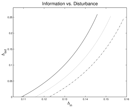
FIG. 2.: The tradeoff between information, $\Delta_{\rm\scriptscriptstyle in}$, and disturbance, $\Delta_{\rm\scriptscriptstyle out}$, is plotted here for $\alpha=1$, $b=0.9$ and three values of $a$. Solid line: $a=0.8$, dotted line: $a=0.79$ and dot-dash line: $a=0.78$ .

$\!\!\!\!\!\!\Delta_{\rm\scriptscriptstyle in}$ will always be maximized by choosing $z=1$ or $z=-1$. However, for $\alpha$ outside of either of those ranges, there will always be a nontrivial tradeoff relation: When Alice’s information gain $\Delta_{\rm\scriptscriptstyle in}$ is maximized, Bob’s information loss $\Delta_{\rm\scriptscriptstyle out}$ will be strictly greater than its minimal value.

The general tradeoff relation, when it exists, is found simply enough by eliminating the variable $z$ from the simultaneous equations (69) and (70). (Two examples of the tradeoff relation are given in figures 2 and 3.) This time—in contrast to what we did in Eq. (75) however—we leave finding the explicit expression as an exercise for the reader: Seeing it explicitly adds little to the analysis already given.

IV Discussion

Our conclusion is straightforward: There are regions in the space of finite-strength efficient measurements without feedback for which a nontrivial information tradeoff relation exists as one unitarily varies around any given fiducial measurement $\cal M$. In a way, it is a shame that we could not make a more unqualified assertion—for instance, that a nontrivial tradeoff relation held for all finite strength quantum measurements without feedback. Indeed the hope that such would be the case was a large part of the motivation for this work.

The question now arises as to the significance of the rather complicated regions defined by Eqs. (79) and (80). What trenchant physical property is implied of a measurement $\cal M$ that sits in the information-disturbance region of a given density operator $\rho$?

A toy idea is that the key distinction lies not in finite vs. infinite measurement strength, but in whether the measurement sits above or below a certain finite-strength

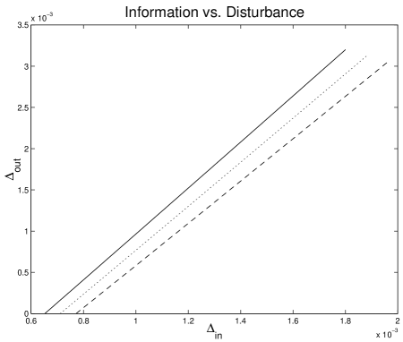
FIG. 3.: The tradeoff between information, $\Delta_{\rm\scriptscriptstyle in}$, and disturbance, $\Delta_{\rm\scriptscriptstyle out}$, is plotted here for $\alpha=1$, $b=0.1$ and three values of $a$. Solid line: $a=0.8$, dotted line: $a=0.79$ and dot-dash line: $a=0.78$ .

threshold. That is to say, in carrying out the program of this paper, we would imagine not only varying over unitary orbits for defining a tradeoff relation, but rather over any region of POVM space so long as a certain constraint on the measurement strength is obeyed. Unfortunately, if this is going to be the case, it is going to require some thinking more subtle than we have carried out so far. This is because for at least one natural definition of measurement strength we again find no nontrivial tradeoff relation. The failure of this program is described in Appendix B. So the question remains.

In general, this paper forms part of a larger effort to fully delimit the information-disturbance tradeoff properties of quantum mechanics.

Appendix A: Efficient Measurements Increase Alice’s Information

In this appendix, we prove that for any efficient quantum measurement, an observer aware of the outcomes will on average increase his “knowledge” of the measured quantum system. More precisely, when a measurement causes the observer to update his density operator from $\rho$ to $\rho_{b}$—as in Eq. (13)—it holds for any concave unitarily invariant function $F$ that

$$F(\rho)\geq\sum_{b}p_{b}F(\rho_{b})\;.$$ (81)

Along the way, and as something of an aside, we will also prove a stronger result that deals directly with relations between the eigenvalues of $\rho$ and all the $\rho_{b}$. This result is most conveniently couched in terms of the mathematical theory of majorization [52], and will require a little notation for its statement.

Let us define $\vec{\lambda}({\cal O})$ to be the vector of eigenvalues of a Hermitian operator $\cal O$ on ${\cal H}_{d}$, with the components arranged in terms of decreasing magnitude. That is to say, let the numbers $\lambda_{i}({\cal O})$ obey the ordering

$$\lambda_{1}({\cal O})\geq\lambda_{2}({\cal O})\geq\cdots\geq\lambda_{d}({\cal O})\;.$$ (82)

We say that a vector $\vec{\lambda}({\cal O})$ is majorized by a vector $\vec{\lambda}({\cal N})$, and write

$$\vec{\lambda}({\cal O})\prec\vec{\lambda}({\cal N})$$ (83)

when

$$\sum_{i=1}^{k}\lambda_{i}({\cal O})\leq\sum_{i=1}^{k}\lambda_{i}({\cal N})$$ (84)

for all $k=1,2,\ldots,d$, and

$$\sum_{i=1}^{d}\lambda_{i}({\cal O})=\sum_{i=1}^{d}\lambda_{i}({\cal N})\;.$$ (85)

One can also say that a Hermitian operator $\cal O$ is majorized by a Hermitian operator $\cal N$, and write ${\cal O}\prec{\cal N}$, when $\vec{\lambda}({\cal O})\prec\vec{\lambda}({\cal N})$, but we will not have any need for that terminology in this development.

Our main result is this:

$$\vec{\lambda}(\rho)\prec\sum_{b}p_{b}\vec{\lambda}(\rho_{b})$$ (86)

(As pointed out before, this result has also been obtained recently in Ref. [37].) The proof of this statement is not too difficult if we rely on some results from the mathematical literature [52], and a method of thought promoted by Ben Schumacher on several occasions to great result—see Refs. [53, 54], to name only a few.

The trick of Schumacher is this. Whenever we have a quantum system $Q$ and we say that it is in a (mixed) state $\rho$, there is nothing to prevent us from thinking that the situation has come about because $Q$ is part of a larger system $RQ$, which we happen to describe via some pure state $|\psi^{\rm\scriptscriptstyle RQ}\rangle$. The state $\rho$ then is just a partial trace over the larger pure state:

$$\rho={\rm tr}_{\rm\scriptscriptstyle R}|\psi^{\rm\scriptscriptstyle RQ}\rangle\langle\psi^{\rm\scriptscriptstyle RQ}|$$ (87)

There are times when such a conception can be quite useful for simplifying the mathematics of a problem. The problem at hand is one of them.

Let us now describe the measurement process on a system $Q$ from such a point of view. It will be useful to make explicit precisely which system we are referring to at any given time: therefore we shall add superscripts or subscripts, $R$, $Q$, or $RQ$ to all density operators to make that clear. In these new terms, the state change under measurement that we are interested in is given by

$$\rho^{\rm\scriptscriptstyle Q}\;\longrightarrow\;\rho^{\rm\scriptscriptstyle Q}_{b}=\frac{1}{p_{b}}U_{b}E_{b}^{1/2}\rho^{\rm\scriptscriptstyle Q}E_{b}^{1/2}U_{b}^{\dagger}$$ (88)

after an outcome $b$ is found. That same measurement, on the other hand, changes the state of the $RQ$ system according to:

$$|\psi^{\rm\scriptscriptstyle RQ}\rangle\;\longrightarrow\;|\psi^{\rm\scriptscriptstyle RQ}_{b}\rangle=\sqrt{\frac{1}{p_{b}}}\,\big{(}I_{\rm\scriptscriptstyle R}\!\otimes A_{b}\big{)}|\psi^{\rm\scriptscriptstyle RQ}\rangle\;,$$ (89)

where

$$A_{b}=U_{b}E_{b}^{1/2}$$ (90)

(Recall that pure states remain pure under an efficient measurement.) The operator $I_{\rm\scriptscriptstyle R}$ in this equation, of course, signifies the identity operator on the $R$ system.

Note that the initial density operators $\rho^{\rm\scriptscriptstyle R}$ and $\rho^{\rm\scriptscriptstyle Q}$ for the $R$ and $Q$ systems are unitarily equivalent. I.e.,

$$\rho^{\rm\scriptscriptstyle R}={\rm tr}_{\rm\scriptscriptstyle Q}|\psi^{\rm\scriptscriptstyle RQ}\rangle\langle\psi^{\rm\scriptscriptstyle RQ}|=V\rho^{Q}V^{\dagger}\;,$$ (91)

for some unitary operator $V$. In particular, it follows that $\rho^{\rm\scriptscriptstyle R}$ and $\rho^{\rm\scriptscriptstyle Q}$ have the same eigenvalues. We can also note, however, that since a measurement on $Q$ can have no overall effect on the $R$, it must be the case that

$$\rho^{\rm\scriptscriptstyle R}={\rm tr}_{\rm\scriptscriptstyle Q}\!\left(\sum_{b}p_{b}|\psi^{\rm\scriptscriptstyle RQ}_{b}\rangle\langle\psi^{\rm\scriptscriptstyle RQ}_{b}|\right).$$ (92)

One can see this more formally by choosing a Schmidt decomposition for $|\psi^{\rm\scriptscriptstyle RQ}\rangle$,

$$|\psi^{\rm\scriptscriptstyle RQ}\rangle=\sum_{k=1}^{d}\sqrt{\lambda_{k}}|r_{k}\rangle|q_{k}\rangle\;.$$ (93)

Then

$${\rm tr}_{\rm\scriptscriptstyle Q} \!\left(\sum_{b}p_{b}|\psi^{\rm\scriptscriptstyle RQ}_{b}\rangle\langle\psi^{\rm\scriptscriptstyle RQ}_{b}|\right)=$$ (101)

$$=\sum_{lb}\langle q_{l}|\big{(}I_{\rm\scriptscriptstyle R}\!\otimes A_{b}\big{)}|\psi^{\rm\scriptscriptstyle RQ}\rangle\langle\psi^{\rm\scriptscriptstyle RQ}|\big{(}I_{\rm\scriptscriptstyle R}\!\otimes A_{b}^{\dagger}\big{)}|q_{l}\rangle$$

$$=\sum_{kmlb}\sqrt{\lambda_{k}}\sqrt{\lambda_{m}}|r_{k}\rangle\langle r_{m}|\langle q_{l}|A_{b}|q_{k}\rangle\langle q_{m}|A_{b}^{\dagger}|q_{l}\rangle$$

$$=\sum_{kmlb}\sqrt{\lambda_{k}}\sqrt{\lambda_{m}}|r_{k}\rangle\langle r_{m}|\langle q_{m}|A_{b}^{\dagger}|q_{l}\rangle\langle q_{l}|A_{b}|q_{k}\rangle$$

$$=\sum_{kmb}\sqrt{\lambda_{k}}\sqrt{\lambda_{m}}|r_{k}\rangle\langle r_{m}|\langle q_{m}|A_{b}^{\dagger}A_{b}|q_{k}\rangle$$

$$=\sum_{km}\sqrt{\lambda_{k}}\sqrt{\lambda_{m}}|r_{k}\rangle\langle r_{m}|\delta_{mk}$$

$$=\sum_{k}\lambda_{k}|r_{k}\rangle\langle r_{k}|$$

$$=\rho^{\rm\scriptscriptstyle R}\;.$$

It follows from Eq. (92) and the statement preceding it that

$$\vec{\lambda}(\rho^{\rm\scriptscriptstyle Q})=\vec{\lambda}(\rho^{\rm\scriptscriptstyle R})=\vec{\lambda}\left({\rm tr}_{\rm\scriptscriptstyle Q}\!\left(\sum_{b}p_{b}|\psi^{\rm\scriptscriptstyle RQ}_{b}\rangle\langle\psi^{\rm\scriptscriptstyle RQ}_{b}|\right)\right).$$ (102)

But ${\rm tr}_{\rm\scriptscriptstyle Q}$ is a linear mapping. So defining

$$\rho^{\rm\scriptscriptstyle R}_{b}={\rm tr}_{\rm\scriptscriptstyle Q}|\psi^{\rm\scriptscriptstyle RQ}_{b}\rangle\langle\psi^{\rm\scriptscriptstyle RQ}_{b}|\;,$$ (103)

we have

$$\vec{\lambda}(\rho^{\rm\scriptscriptstyle Q})=\vec{\lambda}\left(\sum_{b}p_{b}\rho^{\rm\scriptscriptstyle R}_{b}\right)\;.$$ (104)

Now comes the point where we rely on the mathematical literature ever so slightly by using Ky Fan’s dominance theorem [52]. One can show that for any Hermitian operator $\cal O$,

$$\sum_{i=1}^{k}\lambda_{i}({\cal O})=\max_{P}\,{\rm tr}P{\cal O}\;,$$ (105)

where the maximization is taken over all rank-$k$ projectors. It follows from this almost immediately that

$$\vec{\lambda}({\cal O+N})\prec\vec{\lambda}({\cal O})+\vec{\lambda}({\cal N})\;$$ (106)

since

$$\max_{P}\,{\rm tr}P({\cal O+N})\leq\max_{P}\,{\rm tr}P{\cal O}+\max_{P}\,{\rm tr}P{\cal N}\;.$$ (107)

It follows from this that

$$\vec{\lambda}(\rho^{\rm\scriptscriptstyle Q})\prec\sum_{b}\vec{\lambda}(p_{b}\rho^{\rm\scriptscriptstyle R}_{b})=\sum_{b}p_{b}\vec{\lambda}(\rho^{\rm\scriptscriptstyle R}_{b})\;,$$ (108)

since $\vec{\lambda}(c{\cal O})=c\vec{\lambda}({\cal O})$ for any positive number $c$.

Noting finally that the eigenvalue spectrum of $\rho^{\rm\scriptscriptstyle R}_{b}$ is the same as that of $\rho^{\rm\scriptscriptstyle Q}_{b}$, we have ultimately

$$\vec{\lambda}(\rho^{\rm\scriptscriptstyle Q})\prec\sum_{b}p_{b}\vec{\lambda}(\rho^{\rm\scriptscriptstyle Q}_{b})\;.$$ (109)

Stripping off the superscript $Q$, we have the desired result Eq. (86), and the theorem is proved.

It comes about as a corollary to Eq. (86), through some theorems in Ref. [51] that our most desired result—namely Eq. (81)—holds for any concave unitarily invariant function $F$. However, there is a more direct way to see this, and it seems worthwhile to take that route. We need only back up to Eq. (104). From this it follows that

$$F(\rho^{\rm\scriptscriptstyle Q})=F\left(\sum_{b}p_{b}\rho^{\rm\scriptscriptstyle R}_{b}\right)\;.$$ (110)

But, $F$ is concave and so

$$F(\rho^{\rm\scriptscriptstyle Q}) \geq \sum_{b}p_{b}F(\rho^{\rm\scriptscriptstyle R}_{b})$$ (111)

$$= \sum_{b}p_{b}F(\rho^{\rm\scriptscriptstyle Q}_{b})\;.$$ (112)

Again, stripping off the superscript $Q$, we obtain the desired result.

Note Added in Proof: Instructive though it is to derive Eq. (86) by first extending the problem to an ancillary Hilbert space, there is an even shorter route to the result that is worth recording. The trick to note is this: With each efficient measurement ${\cal E}=(E_{b})=(A_{b}^{\dagger}A_{b})$, we can associate a canonical decomposition of the density operator starting from the fact that the $E_{b}$ form a resolution of the identity. Starting from the equation

$$I=\sum_{b}E_{b}\;,$$ (113)

one simply multiplies it from the left and right by $\rho^{1/2}$ to get

$$\rho=\sum_{b}p_{b}\omega_{b}$$ (114)

where

$$\omega_{b}=\frac{1}{p_{b}}\rho^{1/2}E_{b}\rho^{1/2}$$ (115)

and $p_{b}={\rm tr}\rho E_{b}$ as always.

Using the Ky Fan dominance theorem just as before, but now on Eq. (114), we have straight away that

$$\vec{\lambda}(\rho)\prec\sum_{b}p_{b}\vec{\lambda}(\omega_{b})\;.$$ (116)

However, it is an easy matter to see that the operators $\rho^{1/2}E_{b}\rho^{1/2}$ and $A_{b}\rho A_{b}^{\dagger}$ have precisely the same eigenvalue structure. Just start off with the eigenvalue equation

$$\big{(}\rho^{1/2}A_{b}^{\dagger}A_{b}\rho^{1/2}\big{)}|i\rangle=\mu_{i}|i\rangle\;.$$ (117)

Multiplying this from the left by $A_{b}\rho^{1/2}$ and regrouping terms, one gets

$$A_{b}\rho A_{b}^{\dagger}\big{(}A_{b}\rho^{1/2}|i\rangle\big{)}=\mu_{i}\big{(}A_{b}\rho^{1/2}|i\rangle\big{)}\;,$$ (118)

which means that $\rho^{1/2}E_{b}\rho^{1/2}$ and $A_{b}\rho A_{b}^{\dagger}$ have the same eigenvalues. Using this, Eq. (86) follows immediately.

Appendix B: Full Variation over Measurements of a Given Strength

For this Appendix, we drop the distinction of finite vs. infinite measurement strength and attempt to grade all measurements via a single finite number. One possible notion of such a measurement strength is the amount by which Alice’s purity would change if $\rho$ happened to be the maximally mixed state $\frac{1}{2}I$—that is, the measurement strength would be her change of knowledge if she starts out completely ignorant of the system. We can do this with respect to any of the functions $F$ in Eq. (27), but for convenience we will again adopt the impurity $P$ to be the main function of interest. Also for convenience, we will actually adopt two times the said quantity above, i.e., $2\Delta_{\rm\scriptscriptstyle in}(\frac{1}{2}I)$. This choice of pre-factor causes our notion of measurement strength to range in the full interval $[0,1]$.

Thus, using Eq. (69) and taking $a=0$, a given measurement strength $k$ for a two-outcome measurement $(E,I-E)$ is defined by

$$k=\frac{\alpha b^{2}}{2-\alpha}\;.$$ (119)

The question we shall pose in this Appendix is the following. For a given quantum state $\rho$ and a fixed measurement strength $k$, what is the maximum value of $\Delta_{\rm\scriptscriptstyle in}$ and what values of $z$ achieve that maximum? In particular, can we show that the optimal values for $z^{2}$ in this problem are strictly less than 1? Unfortunately, we will have to answer the latter question in the negative, regardless of the value $a$ defining the purity of the initial density operator.

This is seen as follows. Fix $k$ anywhere in the range between 0 and 1. For a fixed $b$ this means that $\alpha$ must take on the value

$$\alpha=\frac{2k}{b^{2}+k}\;.$$ (120)

Note that for a fixed value of $k$ we are not allowed to freely choose $b$ as we wish. This is because for a fixed $k$, the variable $b$ cannot be too small or we would never be able to satisfy Eq. (119). The valid range for $b$ turns out to be

$$k\leq b\leq 1\;.$$ (121)

The consideration leading to this is simple. The function $\frac{\alpha}{2-\alpha}$ is monotonically increasing in $\alpha$. So to find our smallest value of $b$, we should place the largest allowed value of $\alpha$, Eq. (54), into the right-hand side of Eq. (120). Doing this gives Eq. (121).

Plugging Eq. (120) into Eq. (69) gives a surprisingly simple expression

$$\Delta_{\rm\scriptscriptstyle in}=\frac{k(1-a^{2})(1-a^{2}z^{2})b}{2(1+azb)(b-akz)}\;.$$ (122)

Let us now examine the behavior of this as a function of $b$. Taking the partial derivative with respect to $b$, we obtain

$$\frac{2}{k(1-a^{2})(1-a^{2}z^{2})}\,\frac{\partial\Delta_{\rm\scriptscriptstyle in}}{\partial b}\,=\,-\frac{a(b^{2}+k)z}{(1+azb)^{2}(b-akz)^{2}}\;.$$ (123)

Therefore $\Delta_{\rm\scriptscriptstyle in}(b)$ toggles from being an increasing to a decreasing function depending upon the sign of $z$. Thus $\max_{b}\Delta_{\rm\scriptscriptstyle in}(b)$ takes on a piecewise form. If $z\geq 0$, we should choose $b=k$; if $z\leq 0$, we should choose $b=1$. The resultant of these choices is conveniently summarized as follows:

$$\Delta_{\rm\scriptscriptstyle in}^{\!\rm\scriptscriptstyle max}(z)=\frac{1}{2}k(1-a^{2})\frac{1+a|z|}{1+ak|z|}\;.$$ (124)

The function $\Delta_{\rm\scriptscriptstyle in}^{\!\rm\scriptscriptstyle max}(z)$ in Eq. (124) is increasing in $|z|$ since $k\leq 1$. Hence it finally follows that the very best strategy on Alice’s part for a given measurement strength $k$ is to take $z=1$ or $-1$. Doing so gives her an absolute maximum purity change of

$$\Delta_{\rm\scriptscriptstyle in}^{\!\rm\scriptscriptstyle max}=\frac{1}{2}k(1-a^{2})\frac{1+a}{1+ak}\;,$$ (125)

and that purity change is accompanied by a purity change of $\Delta_{\rm\scriptscriptstyle out}=0$ for Bob.

REFERENCES

- [1] A. Einstein, B. Podolsky, and N. Rosen, Phys. Rev. 47, 777–780 (1935).
- [2] N. Bohr, Phys. Rev. 48, 696–702 (1935).
-
[3]
We should point out that lately it has become fashionable to say
that Bohr dropped his rhetoric of “measurement causing
disturbance” soon after his reply to the EPR paper
[4]. We disagree with this as the counter-evidence
is easily exhibited in almost everything that Bohr wrote on the
subject thereafter. A prime example is this passage from
Ref. [5].
The very fact that quantum phenomena cannot be analysed on classical lines thus implies the impossibility of separating a behavior of atomic objects from the interaction of these objects with the measuring instruments which serve to specify the conditions under which the phenomena appear. In particular, the individuality of the typical quantum effects finds proper expression in the circumstance that any attempt at subdividing the phenomena will demand a change in the experimental arrangement, introducing new sources of uncontrollable interaction between objects and measuring instruments
- [4] N. D. Mermin, private communication, 19 May 2000.
- [5] N. Bohr, Dialectica 2, 312–318 (1948).
- [6] W. Pauli, Writings on Philosophy and Physics, edited by C. P. Enz and K. von Meyenn, (Springer-Verlag, Berlin, 1995), p. 132.
- [7] M. Jammer, The Philosophy of Quantum Mechanics: The Interpretations of Quantum Mechanics in Historical Perspective, (Wiley, New York, 1974).
- [8] M. Beller, Quantum Dialogue: The Making of a Revolution, (U. of Chicago Press, Chicago, 1999).
- [9] We pay no attention to variants of quantum mechanics, such as Bohmian mechanics, that incorporate nonlocal hidden variables.
- [10] For a clear discussion of this point, see N. D. Mermin, Boojums All the Way Through: Communicating Science in a Prosaic Age, (Cambridge U. Press, Cambridge, 1990), pp. 110–176.
- [11] A. Peres, Phys. Rev. A 61, 022116-1–022116-9 (2000).
- [12] C. A. Fuchs and A. Peres, Phys. Today 53(3), 70–71 (2000).
- [13] S. L. Braunstein and C. M. Caves, Found. Phys. Lett. 1, 3–12 (1988).
- [14] W. Heisenberg, in Quantum Theory and Measurement, edited by J. A. Wheeler and W. H. Zurek (Princeton U. Press, Princeton, NJ, 1983), pp. 62–84.
- [15] W. G. Unruh, Phys. Rev. D 18, 1764–1772 (1978); 19, 2888–2896 (1979).
- [16] K. Kraus, States, Effects, and Operations: Fundamental Notions of Quantum Theory, (Springer-Verlag, Berlin, 1983).
- [17] The first appearance of this idea seems to be in the work of Stephen Wiesner circa 1970, but remained unpublished until much later. See S. Wiesner, SIGACT News 15, 78–88 (1983).
- [18] C. H. Bennett and G. Brassard, in Proc. IEEE International Conference on Computers, Systems and Signal Processing, Bangalore, India, December 10-12, 1984, (IEEE Press, New York, 1984), pp. 175–179.
- [19] C. H. Bennett, G. Brassard, and N. D. Mermin, Phys. Rev. Lett. 68, 557–559 (1992).
- [20] C. H. Bennett, Phys. Rev. Lett. 68, 3121–3124 (1992).
- [21] C. A. Fuchs, Fort. der Phys. 46, 535–565 (1998).
- [22] C. A. Fuchs and A. Peres, Phys. Rev. A 53, 2038–2045 (1996).
- [23] C. A. Fuchs, N. Gisin, R. B. Griffiths, C.-S. Niu, and A. Peres, Phys. Rev. A 56, 1163–1172 (1997).
- [24] D. Bruss, Phys. Rev. Lett. 81, 2598–2601 (1998).
- [25] H. E. Kyburg, Jr. and H. E. Smokler, eds., Studies in Subjective Probability, Second Edition, (Robert E. Krieger Publishing, Huntington, NY, 1980).
- [26] J. M. Bernardo and A. F. M. Smith, Bayesian Theory, (Wiley, New York, 1994).
- [27] One of the authors (CAF) is tempted to speculate that this idea alone (suitably refined) captures the essence of quantum mechanics. The formalism of quantum theory, by this view, is simply the best agreement we can all come to in a world so sensitive to our experimental interventions. This contrasts with the defining property of the classical world, which, at the outset, is assumed describable by a set of variables stable enough that we can discover them or, at the very least, safely contemplate their supposed existence.
- [28] A. M. Gleason, J. Math. Mech. 6, 885–894 (1957).
- [29] R. B. Ash, Information Theory, (Dover, New York, 1965).
- [30] A. Wehrl, Rev. Mod. Phys. 50, 221–259 (1978).
- [31] W. K. Wootters and B. D. Fields, Ann. Phys. 191, 363–381 (1989).
- [32] W. K. Wootters, Found. Phys. 20, 1365–1378 (1990).
- [33] K. R. W. Jones, J. Phys. A 24, 1237–1244 (1991).
- [34] G. Lüders, Ann. der Phys. 8, 323–328 (1951).
- [35] P. Busch, P. Lahti, and P. Mittelstaedt, The Quantum Theory of Measurement, Second revised edition, (Springer-Verlag, Berlin, 1996).
- [36] P. Busch and J. Singh, Phys. Lett. A 249, 10–12 (1998).
- [37] M. A. Nielsen, “Characterizing Mixing and Measurement in Quantum Mechanics,” quant-ph/0008073.
- [38] A. Peres, Quantum Theory: Concepts and Methods, (Kluwer, Dordrecht, 1993).
- [39] H.M. Wiseman and G.J. Milburn, Phys. Rev. A 47, 642 (1993).
- [40] R. Schatten, Norm Ideals of Completely Continuous Operators, (Springer-Verlag, Berlin, 1960).
- [41] H. N. Barnum, Quantum Information Theory, Ph. D. Thesis, University of New Mexico, Albuquerque, NM, 1998, Chap. 4.
- [42] K. Banaszek, “Fidelity Tradeoff in Quantum Operations,” LANL e-print archive, quant-ph/0003123.
- [43] A. C. Doherty, K. Jacobs, and G. Jungman, “Information, Disturbance, and Hamiltonian Quantum Feedback Control,” quant-ph/0006013.
- [44] A. Fujiwara and H. Nagaoka, IEEE Trans. Inf. Theory 44, 1071–1086 (1998).
- [45] R. G. Gallager, Information Theory and Reliable Communication, (Wiley, New York, 1968).
- [46] R. Jozsa, D. Robb, and W. K. Wootters, Phys. Rev. A 49, 668-677 (1994).
- [47] C. M. Caves and C. A. Fuchs, in The Dilemma of Einstein, Podolsky and Rosen – 60 Years Later, Ann. Israel Phys. Soc. 12, edited by A. Mann and M. Revzen, 226–257 (1996).
- [48] E. T. Jaynes, Phys. Rev. 106, 620–630 (1957).
- [49] J. Aczél and Z. Daróczy, On Measures of Information and Their Characterizations, (Academic Press, New York, 1975).
- [50] M. A. Nielsen also makes a similar point in Ref. [37].
- [51] T. Ando, Lin. Alg. App. 118, 163–248 (1989).
- [52] A. W. Marshall and I. Olkin, Inequalities: Theory of Majorization and Its Applications, (Academic Press, New York, 1979).
- [53] B. W. Schumacher, Phys. Rev. A 54, 2614–2628 (1996).
- [54] N. Linden, S. Popescu, B. Schumacher, and M. Westmoreland, “Reversibility of Local Transformations of Multiparticle Entanglement,” quant-ph/9912039.