A Family of Grover’s Quantum Searching Algorithms

Abstract

We introduce the concepts of Grover operators and Grover kernels to systematically analyse Grover’s searching algorithms. Then, we investigate a one-parameter family of quantum searching algorithms of Grover’s type and we show that the standard Grover’s algorithm is a distinguished member of this family. We show that all the algorithms of this class solve the searching problem with an efficiency of order $O(\sqrt{N})$, with a coefficient which is class-dependent. The analysis of this dependence is a test of the stability and robustness of the algorithms. We show the stability of this constructions under perturbations of the initial conditions and extend them upon a very general class of Grover operators.

PACS number: 03.67.Lx, 03.67.-a

]

I Introduction

The problem of searching an element in a list of $N$ unsorted elements when this number becomes very large is known to be one of the basic problems in Computational Science. Classically, one may devise many strategies to perform that search, but if the elements in the list are distributed with equal probability, then we shall need to make $O(N)$ trials in order to have a high confidence of finding the desired element, also called marked element. The formulation of quantum computation as a well-stablished theoretical discipline for storing and processing information [1] has opened the possibility of designing new searching algorithms with no classical analogue. The familiar Grover quantum searching algorithm takes advantage of the quantum mechanical properties to perform the searching problem with an efficiency of order $O(\sqrt{N})$ [2], [3].

In classical computation there exist design techniques which provide general directions for algorithmic problem solving. In quantum computation however, the list of quantum algorithms is very short. It seems we are lacking the basic principles underlying the quantum algorithmic design. Under these circumstances it is a good choice to put to the test the currently known quantum algorithms. In this work our purpose is to follow this goal with Grover’s quantum searching algorithm by trying to understand the relevant pieces of this algorithm and wondering to what extent they allow for generalization [4], [5], [6], [7], [8], [9].

Let us state the searching problem in terms of a list ${\cal L}[0,1,\ldots,N-1]$ with a number $N$ of unsorted elements. We shall denote by $x_{0}$ the marked element in ${\cal L}$ that we are searching for. The quantum mechanical solution of this searching problem goes through the preparation of a quantum register in a quantum computer to store the $N$ items of our list. This is how quantum parallelism is realized. Thus, let us assume that our quantum registers are made of $n$ qubits so that the total elements we have are $N=2^{n}$. Let us denote by $|x\rangle$, $x=0,1,\ldots,N-1$ the ket states of the computational basis which are orthonormalized. Any state $|\Psi\rangle$ of the quantum register is a linear superposition of the computational states. In the beginning of the algorithm the quantum register is initialized to a given quantum state $|\Psi\rangle=|x_{\rm in}\rangle$.

The second component of the algorithm is to design a quantum operation which will be repeatedly applied to $|x_{\rm in}\rangle$ in order to find the marked element. This strategy is similar to the classical counterpart algorithm. The difference is the fact that the quantum operation is realized in terms of an unitary operator which implements the reversible quantum computation. It is this quantum operation what has been so neatly designed by Grover [2]. With Grover’s choice we may say that the quantum evolution is such that the constructive interference of quantum amplitudes is directed towards the marked state one looks for.

II Grover Operators

In order to set up our analysis we shall need to introduce some definitions.

Definition 1 A Grover operator $G$ is any unitary operator with at most two different eigenvalues; i.e., $G$ a linear superposition of two orthogonal projectors $P$ and $Q$:

$$G=\alpha P+\beta Q,\;\;P^{2}=P,\;Q^{2}=Q,\;\;P+Q=1$$ (1)

where $\alpha,\beta\in{\bf C}$ are complex numbers of unit norm.

Definition 2 A Grover kernel $K$ is the product of two Grover operators:

$$K=G_{2}G_{1}$$ (2)

Some elementary properties follow immediately from these definitions.

Property 1 Any Grover kernel $K$ is a unitary operator, and therefore, it can be used to implement the unitary evolution in a quantum computer.

Property 2 Let the Grover operators $G_{1},G_{2}$ be chosen such that

$$G_{1}=\alpha P_{x_{0}}+\beta Q_{x_{0}},\quad P_{x_{0}}=|x_{0}\rangle\langle x_{0}|,\;P_{x_{0}}+Q_{x_{0}}=1$$ (3)

$$G_{2}=\gamma\bar{P}+\delta\bar{Q},\quad\bar{P}+\bar{Q}=1$$ (4)

with $\bar{P}$ given by the rank 1 matrix

$$\bar{P}={1\over N}\left(\begin{array}[]{ccc}1&\ldots&1\\ \vdots&&\vdots\\ 1&\ldots&1\end{array}\right)$$ (5)

This is clearly a projector $\bar{P}=|k_{0}\rangle\langle k_{0}|$ on the subspace spanned by the state $|k_{0}\rangle={1\over\sqrt{N}}(1,\ldots,1)^{\rm t}$, where the superscript denotes the transpose. Then, if we take the following set of parameters,

$$\alpha=-1,\;\beta=1,\;\gamma=-1,\;\delta=1$$ (6)

the Grover kernel (2) reproduces the original Grover’s choice. This property follows inmediately by construction. In fact, we have in this case $G_{1}=1-2P_{x_{0}}=:G_{x_{0}}$ whilst the operator $G_{2}=1-2\bar{P}$ coincides with the diffusion operator introduced by Grover to implement the inversion about the average [2].

One can also show the following property which provides a geometrical meaning for the Grover kernels.

Property 3 Let ${\cal K}_{\rm G}$ denote the set of all the Grover kernels for fixed $\{|x_{0}\rangle,|k_{0}\rangle\}$. Then ${\cal K}_{\rm G}$ can be viewed as a 3D-subset of the group U(2) which is of the form $S^{1}\times{\cal K}_{\rm G}^{\prime}$, where ${\cal K}_{\rm G}^{\prime}$ is a 2D-submanifold of SU(2) (Fig.1).

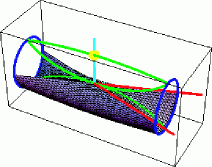
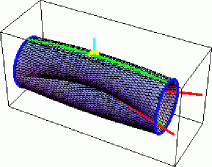
FIG. 1.: Left: half of the surface ${\cal K}_{\rm G}^{\prime}$ for $N=10$. Right: the whole surface ${\cal K}_{\rm G}^{\prime}$ for $N=10$. In red, the rotation axes corresponding to ${\rm i}G_{1,2}\in SU(2)$. In pale blue, the normal to their plane. The yellow dot signals the original Grover kernel. The blue curves are the border $\alpha=\pi,3\pi$, where $\alpha$ is the rotation angle. In green, the locus of kernels $K$ with factors ${\rm i}G_{1,2}$ with the same rotation angles mod $2\pi$.

The content of this property is illustrated in Fig.1. It follows from the fact that the two parameters of a Grover kernel in Definition 2 with the fixing (6) can be used to parametrize a subset of the unitary group $U(2)$ of complex $2\times 2$ matrices. This 3D-subset has a factorized form $S^{1}\times{\cal K}_{\rm G}^{\prime}$ where $S^{1}$ is the unit circle (the group U(1) and we call ${\cal K}_{\rm G}^{\prime}$ a certain 2D-submanifold of the group of special unitary matrices SU(2) whose construction we explain in the following and we plot in Fig.1. This figure is constructed by parametrizing the two elements $\pm{\rm i}G_{1,2}$ of SU(2) as follows, $\pm{\rm i}G_{1,2}={\rm e}^{{\rm i}\alpha_{1,2}{\bf n}_{1,2}\cdot\mathbf{\sigma}}$, where $\mathbf{\sigma}$ are the Pauli matrices and ${\bf n}_{1,2}$ are unit vectors which are kept fixed. Likewise, we parametrize the corresponding Grover kernel (2) as $K={\rm e}^{{\rm i}\alpha{\bf n}\cdot\mathbf{\sigma}}$. Then, upon varying the parameters $\alpha_{1,2}$ we obtain the surface depicted in Fig.1

Let us point out the following interpretation of the Grover operators. Let us think of the computational basis $\{|x\rangle\}$ as a coordinate basis in Quantum Mechanics and introduce the quantum discrete Fourier transform in the standard fashion, $|\hat{x}\rangle:=U_{\rm DFT}|x\rangle={1\over\sqrt{N}}\sum_{y=0}^{N-1}{\rm e}^{2\pi{\rm i}x\cdot y/N}|y\rangle$. The transformed basis $\{|\hat{x}\rangle\}$ can then be seen as the dual momentum basis. Then, it is easy to see that in such a basis the projector operator $\bar{P}$ takes the following form:

$$U_{\rm DFT}^{-1}\bar{P}U_{\rm DFT}=|0\rangle\langle 0|=:P_{0}$$ (7)

This means that the Grover operator $G_{2}$ takes the same matricial form in the momentum basis as the Grover operator $G_{1}$ in the coordinate basis. They are somehow dual of each other. The original Grover kernel takes then the form

$$K=U_{\rm DFT}G_{x=0}U_{\rm DFT}^{-1}G_{x_{0}}$$ (8)

which shows that a Grover kernel has a part local in coordinate space and anoter part which is local in momentum space.

This “momentum” interpretation of the search algorithm stems from a quantum mechanical analogy between the computational basis and its Fourier transformed states which enter the definition of the Grover operators. We would like to point out that similar analogies have been used in connection with alternative formulations of the quantum searching algorithm, namely, the analog analogue of a digital quantum computation with Grover’s algorithm [10] which is based in a Hamiltonian formulation.

III The Searching Algorithms

A The Basic Formalism

Next, the third part of the algorithms corresponds to applying the Grover kernel $K$ to the initial state $|x_{\rm in}\rangle$ a number of times $m$ seeking a final state $|x_{\rm f}\rangle$ given by

$$|x_{\rm f}(m)\rangle=K^{m}|x_{\rm in}\rangle$$ (9)

such that the probability ${\cal P}(x_{0})$ of finding the marked state is above a given threshold value. We shall take this value to be $1/2$, meaning that we choose a probability of success of $50\%$ or larger. Thus, we are seeking under which circumstances the following condition

$${\cal P}(x_{0})=|\langle x_{0}|K^{m}|x_{\rm in}\rangle|^{2}>1/2$$ (10)

holds true.

The analysis of this probability gets simplified if we realize that the evolution associated to the searching problem can be mapped onto a reduced 2D-space spanned by the vectors

$$\{|x_{0}\rangle,|x_{\perp}\rangle:={1\over{\sqrt{N-1}}}\sum_{x\neq x_{0}}|x\rangle\}$$ (11)

Then we can easily compute the projections of the Grover operators $G_{1},G_{2}$ in the reduced basis with the result

$$G_{1}=\left(\begin{array}[]{cc}\alpha&0\\ 0&\beta\end{array}\right)$$ (12)

$$G_{2}=\left(\begin{array}[]{cc}\delta&0\\ 0&\gamma\end{array}\right)+(\gamma-\delta)\left(\begin{array}[]{cc}{1\over N}&{\sqrt{N-1}\over N}\\ {\sqrt{N-1}\over N}&{-1\over N}\end{array}\right)$$ (13)

From now on, we shall fix two of the phase parameters using the freedom we have to define each Grover factor in (2) up to an overall phase. Then we decide to fix them as follows:

$$\alpha=\gamma=-1$$ (14)

With this choice, the Grover kernel (2) takes the following form in this basis:

$$K={1\over N}\left(\begin{array}[]{cc}1+\delta(1-N)&-\beta(1+\delta)\sqrt{N-1}\\ (1+\delta)\sqrt{N-1}&\beta(1+\delta-N)\end{array}\right)$$ (15)

We shall fix the initial conditions using the same initial state $|x_{\rm in}\rangle$ as in the original Grover’s algorithm [2], i.e., we choose the uniform state corresponding to zero momentum and find its components in the reduced basis to be

$$|x_{\rm in}\rangle={1\over{\sqrt{N}}}|x_{0}\rangle+\sqrt{{N-1\over N}}|x_{\perp}\rangle$$ (16)

In order to compute the probability amplitude in (10), we introduce the spectral decomposition of the Grover kernel $K$ in terms of its eigenvectors $\{|\kappa_{1}\rangle,|\kappa_{2}\rangle\}$, with eigenvalues ${\rm e}^{{\rm i}\omega_{1}},{\rm e}^{{\rm i}\omega_{2}}$. Thus we have

$$\begin{split}&{\cal A}(x_{0}):=\langle x_{0}|K^{m}|x_{\rm in}\rangle=\\ &{1\over\sqrt{N}}\sum_{j=1}^{2}\left\{|\langle x_{0}|\kappa_{j}\rangle|^{2}+{\sqrt{N-1}}\langle x_{0}|\kappa_{j}\rangle\langle\kappa_{j}|x_{\perp}\rangle\right\}{\rm e}^{{\rm i}m\omega_{j}}\end{split}$$ (17)

This in turn can be casted into the following closed form:

$$\begin{split}&\langle x_{0}|K^{m}|x_{\rm in}\rangle=\\ &{\rm e}^{{\rm i}m\omega_{1}}\left({1\over\sqrt{N}}+({\rm e}^{{\rm i}m\Delta\omega}-1)\langle x_{0}|\kappa_{2}\rangle\langle\kappa_{2}|x_{\rm in}\rangle\right)\end{split}$$ (18)

with $\Delta\omega=\omega_{2}-\omega_{1}$.

In terms of the matrix invariants

$${\rm Det}K=\beta\delta,\quad{\rm Tr}K=-(\beta+\delta)+(1+\beta)(1+\delta){1\over N}$$ (19)

the eigenvalues $\zeta_{1,2}={\rm e}^{{\rm i}\omega_{1,2}}$ are given by

$$\zeta_{1,2}=({\rm Tr}K)/2\mp\sqrt{-{\rm Det}K+({\rm Tr}K/2)^{2}}$$ (20)

The corresponding unnormalized eigenvectors are

$$|\kappa_{1,2}\rangle\propto\left(\begin{array}[]{c}{A\mp\sqrt{-4({\rm Det}K)N^{2}+A^{2}}\over 2(1+\delta)\sqrt{N-1}}\\ 1\end{array}\right)$$ (21)

with

$$A:=(\beta-\delta)N+(1-\beta)(1+\delta)$$ (22)

Although we could work out all the expressions for a generic value $N$ of elements in the list, we shall restrict our analysis to the case of a large number of elements, $N\rightarrow\infty$, and we shall leave for a numerical simulation the effect of arbitrary $N$. Thus, in this asymptotic limit we need to know the behaviour for $N\gg 1$ of the eigenvector $|\kappa_{2}\rangle$ which turns out to be

$$|\kappa_{2}\rangle\propto\left(\begin{array}[]{c}{\beta-\delta\over 1+\delta}\sqrt{N}+O({1\over\sqrt{N}})\\ 1\end{array}\right)$$ (23)

Thus, for generic values of $\beta,\delta$ we observe that the first component of the eigenvector dominates over the second one meaning that asymtoptically $|\kappa_{2}\rangle\sim|x_{0}\rangle$ and then $\langle x_{0}|\kappa_{2}\rangle\langle\kappa_{2}|x_{\rm in}\rangle=O({1\over\sqrt{N}})$. This implies that the probability of success in (18) will never reach the threshold value (10). Then we are forced to tune the values of the two parameters in order to have a well-defined and nontrivial algorithm and we demand

$$\beta=\delta\neq-1$$ (24)

Now the asymptotic behaviour of the eigenvector changes and is given by a balanced superposition of marked and unmarked states, as follows

$$|\kappa_{2}\rangle\sim{1\over\sqrt{2}}\left(\begin{array}[]{c}{\rm i}\delta^{1/2}\\ 1\end{array}\right)$$ (25)

This is normalized and we see that none of the components dominates. When we insert this expression into (18) we find

$$|\langle x_{0}|K^{m}|x_{\rm in}\rangle|\sim{|\delta|\over 2}|{\rm e}^{{\rm i}m\Delta\omega}-1|\sim\left|\sin({m\Delta\omega\over 2})\right|$$ (26)

This expression means that we have succeded in finding a class of algorithms which are apropriate for solving the quantum searching problem. Now we need to find out how efficient they are. To do this let us denote by $M$ the values of the time step $m$ at which the probability becomes maximum; then

$$M=\lfloor\left|\pi/\Delta\omega\right|\rfloor$$ (27)

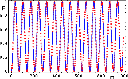
FIG. 2.: Probability of success ${\cal P}$ as a function of the time step for $N=1000$ and $\beta=\delta={\rm e}^{{\rm i}\pi/2}$.

As it happens, we are interested in the asymptotic behaviour of this optimal periods of time $M$. From the equation (20) we find the following behaviour as $N\rightarrow\infty$:

$$\Delta\omega\sim{4\over\sqrt{N}}{\rm Re}\sqrt{\delta}$$ (28)

Thus, if we parametrize $\delta={\rm e}^{{\rm i}\phi}$, then we finally obtain the expression,

$$M\sim\left\lfloor{\pi\over 4\cos{\phi\over 2}}\sqrt{N}\right\rfloor$$ (29)

Therefore, we conclude that the Grover algorithm of the class parametrized by $\phi$ is a well-defined quantum searching algorithm with an efficiency of order $O(\sqrt{N})$ and with a subdominant behaviour which depends on each element of the family. Within this class, the original Grover algorithm is a distinguished element for which the coefficient in (29) achieves its optimal value at $\phi=0$. Moreover, the worst value occurs for $\phi\to\pi$; in this limit $M$ is not well-defined, and it corresponds to trivial case where the Grover kernel is just the identity operator, $K=1$.

The expression (29) for $M$ can also be given another meaning regarding the stability of the Grover’s case $\phi=0$. It is plain that under a small perturbation $\delta\phi$ around this value, its optimal nature is not spoiled in first order for we find a behaviour which is quadratic in the perturbation, namely, $M\sim{\pi\over 4}(1+0.125(\delta\phi)^{2})\sqrt{N}$. This stability considered here is with respect to perturbations in eigenvalues (or eigenvectors) in the reduced 2-dimensional subspace specified by the quantum searching problem (11). We also require these type of perturbations to hold in all iterations.

Howewer, if we happen to choose a Grover kernel with a $\phi$ far from $0$ we may end up with a searching algorithm for which the leading behaviour order $O(\sqrt{N})$ is masqueraded by the big value of the coefficient and the time to achive a succedding probability becomes very large. For instance, we may have a Grover kernel with a behaviour $M\sim 10^{3}\sqrt{N}$ and for a value of $N=10^{6}$ it would turn out as efficient as a classical algorithm of order $O(N)=10^{6}$. Thus, the limit $\phi\rightarrow\pi$ behaves as a sort of classical limit where the quantum properties disappear.

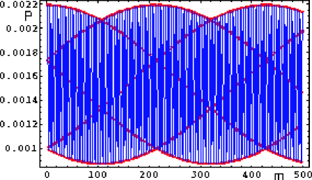
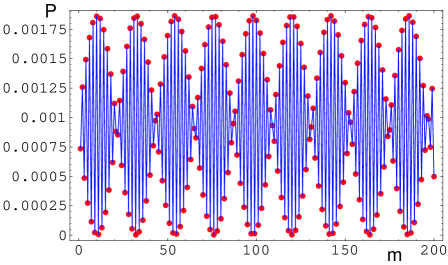
FIG. 3.: Probability of success ${\cal P}$ as a function of the time step for $N=1000$ and $\beta={\rm i},\delta={\rm i}{\rm e}^{{\rm i}5/4}$ (up), $\beta={\rm i},\delta={\rm i}{\rm e}^{{\rm i}3}$ (down).

In Fig. 2 we have plotted the probability of success as a function of the time step $m$ for a list of $N=1000$ elements and a choice of parameters $\beta=\delta={\rm e}^{{\rm i}\pi/2}$ satisfying condition (24). We observe how the algorithm is fully efficient in achieving the maximum probability possible. Despite $\phi=\pi/2$ is not close to Grover’s optimal value of $0$, we find an excellent behaviour. The main difference with the optimal case is that here the number of maxima is $14$ while for Grover’s it is $20$, as implied by (29). This looks like a pattern of fully constructive interference.

In Fig. 3 we have plotted the same function but with a choice of parameters $\beta={\rm i},\delta={\rm i}{\rm e}^{{\rm i}5/4}$ ($\beta={\rm i},\delta={\rm i}{\rm e}^{{\rm i}3}$) violating condition (24). We observe how the algorithm becomes inefficient and the maximum it takes is lesser than $0.0021923$ ($0.001864$) for any time step. This looks like a pattern of partially constructive interference.

We find this behaviour as reminiscent of a quantum phase transition where the transition is driven by quantum fluctuations instead of standard thermal fluctuations. In this type of transition each quantum phase is characterized by a ground state which is different in each phase. It is the variation of a coupling constant in the Hamiltonian of the quantum many-body problem which controls the occurrence of one quantum phase or another in the same manner as the temperature does the job in thermal transitions. In our case we may consider the two different asymptotic behaviours of the eigenvector $|\kappa_{2}\rangle$ as playing the role of two ground states. Following this analogy, we may see our family of algorithms parametrized by a torus ${\cal T}=S^{1}\times S^{1}$ where the parameters $\beta$ and $\delta$ take their values and the difference $g:=\beta-\delta$ is a sort of coupling constant which governs in which of the two phases we are. When $g\neq 0$ we fall into a sort of disordered phase where the efficiency of this class of Grover’s algorithms is spoiled. However, when $g=0$ we are located precisely at one equal superposition of the pricipal cycles of the torus which defines a one-parameter family of efficient algorithms.

B The Influence of Initial Conditions

Next we shall address the issue of to what extent this one-parameter family of algorithms depends on the choice of initial conditions for the initial state $|x_{\rm in}\rangle$. We would like to check that the stable behaviour we have found is not disturbed under perturbations of initial conditions.

Let us consider a more general initial state $|x_{\rm in}\rangle$ which is not the precise one used in the original Grover’s algorithm [2] but instead it is chosen as

$$|x_{\rm in}\rangle={a\over{\sqrt{N}}}|x_{0}\rangle+b\sqrt{{N-1\over N}}|x_{\perp}\rangle$$ (30)

where $a$ and $b$ are chosen to satisfy a normalization condition. Then, it is possible to go over the previous analysis and find that the probability amplitude is now given by

$$\begin{split}&\langle x_{0}|K^{m}|x_{\rm in}\rangle=\\ &{\rm e}^{{\rm i}m\omega_{1}}\left({a\over\sqrt{N}}+({\rm e}^{{\rm i}m\Delta\omega}-1)\langle x_{0}|\kappa_{2}\rangle\langle\kappa_{2}|x_{\rm in}\rangle\right)\end{split}$$ (31)

where now $|x_{\rm in}\rangle$ is the new initial state (30). We have to distinguish two cases: i) The coefficient $a$ of the marked state is order 1 and ii) it is order bigger than 1, say of order $O(\sqrt{N})$. In the latter case ii), it means that the initial state is so peaked around the marked state that we do not even need to resort to a searching algorithm, but instead measure directly on the initial state to find sucessfully the marked state. Thus, we shall restrict to case i) in the following. Now the key point is to realize that all the previous asymptotic analysis is dominated by the behaviour of the eigenvector $|\kappa_{2}\rangle$ given by expression (23) which is something intrinsic to the Grover kernel and independent of the initial conditions. Thus, if condition (24) is not satisfied, then as we are in case i) the first term in the RHS of (31) is not relevant and we are led again to the conclusion that the algorithm is not efficient. On the contrary, if condition (24) is satisfied the same mechanism based on (25) operates again and the algorithm has a probability of success measured by

$$|\langle x_{0}|K^{m}|x_{\rm in}\rangle|\sim|b|\sin({m\Delta\omega\over 2})$$ (32)

with $\Delta\omega$ also given by (28). Then we may conclude that the class of algorithms is stable under perturbations of the initial conditions.

C Extended Formalism

Finally, we would like to check how general is this construction in terms of projection operators of the type used in (5) for $\bar{P}$. To this end let us recall that $\bar{P}$ can be interpreted as the projector $|\hat{0}\rangle\langle\hat{0}|$. Thus a natural generalization is to consider a projector on a different momentum state, say $|\hat{y}_{0}\rangle$, with $y_{0}\neq 0$. The matrix elements of this projection operator in the coordinate basis are

$$(\bar{P})_{x,x^{\prime}}={1\over N}{\rm e}^{2\pi{\rm i}(x^{\prime}-x)\cdot y_{0}/N},\quad x,x^{\prime}=0,1,\ldots,N-1$$ (33)

We can go even further and consider a general form for the states $|x_{0}\rangle,|x_{\perp}\rangle,|k_{0}\rangle$ as follows,

$$\begin{split}&|x_{0}\rangle=(1,0,\ldots,0)^{\rm t}\\ &|x_{\perp}\rangle={1\over\sqrt{1-\alpha_{1}^{2}}}(0,\alpha_{2},\ldots,\alpha_{N})^{\rm t}\\ &|k_{0}\rangle=(\alpha_{1},\alpha_{2},\ldots,\alpha_{N})^{\rm t}\end{split}$$ (34)

where there is no loss of generality by chosing $|x_{0}\rangle$ in this way; $\alpha_{1},\ldots,\alpha_{N}$ is a given and normalized set of arbitrary complex amplitudes, with $\alpha_{1}>0$. We will assume that $||\alpha||^{2}>\alpha_{1}^{2}$.

The projector $\bar{P}$ is chosen to be

$$\bar{P}=|k_{0}\rangle\langle k_{0}|$$ (35)

and it admits (33) as a particular case.

Now in the reduced 2D-basis spanned by $\{|x_{0}\rangle,|x_{\perp}\rangle\}$ the Grover kernel has the following expression:

$$K=\left(\begin{array}[]{cc}-\delta+\Delta\alpha_{1}^{2}&-\beta\Delta\alpha_{1}\sqrt{1-\alpha_{1}^{2}}\\ \Delta\alpha_{1}\sqrt{1-\alpha_{1}^{2}}&\beta(\Delta\alpha_{1}^{2}-1)\end{array}\right)$$ (36)

with $\Delta:=1+\delta$. Thus all the dynamics depends on the relative strength of the real amplitude $\alpha_{1}$ with respect to the rest of the amplitudes. If we set $\alpha_{i}=1/\sqrt{N}$ $\forall i$, then we recover the same expression as in (15). Moreover, the initial condition is taken as

$$|x_{\rm in}\rangle=\alpha_{1}|x_{0}\rangle+\sqrt{1-\alpha_{1}^{2}}|x_{\perp}\rangle$$ (37)

In order to perform our analysis, we shall assume that the unknown amplitude $\alpha_{1}$ behaves generically as $\alpha_{1}\sim 1/\sqrt{N}$, and consequently $\sqrt{1-\alpha_{1}^{2}}\sim\sqrt{1-1/N}$. Under these circumstances, we find the following asymptotic behaviour for the eigenvector $|\kappa_{2}\rangle$ of the Grover kernel: if $\beta\neq\delta$ and $\delta\neq-1$,

$$|\kappa_{2}\rangle\propto\left(\begin{array}[]{c}{\beta-\delta\over 1+\delta}{1\over\alpha_{1}}\\ 1\end{array}\right)$$ (38)

and if $\beta=\delta$,

$$|\kappa_{2}\rangle\sim{1\over\sqrt{2}}\left(\begin{array}[]{c}{\rm i}\delta^{1/2}\\ 1\end{array}\right)$$ (39)

This latter case is again the only favorable to obtain an efficient algorithm and the behaviour of the time $M$ for achieving maximum probability of success takes the following form

$$M\sim{\pi\alpha_{1}^{-1}\over 4\cos{\phi\over 2}}$$ (40)

We conclude then that our construction of quantum searching algorithms of Grover’s type are general enough under different choices of Grover operators $G_{1},G_{2}$ and that the analyisis performed with the simplest choice of these operators captures the essential properties of the class of algorithms we have presented.

IV Conclusions

We have introduced the notion of Grover operators and Grover kernels which lead to a systematic study of Grover’s quantum searching algorithms. These notions facilitates the generalization of Grover’s algorithms in several direcctions. We have characterized the basic features of these algorithms in terms of these operarators whose main properties we have established in Sect. II. Using these operators we have investigated a family of Grover kernels whose qualities as efficient algorithms depend on the range of parameters entering the construction of their associated Grover operators. When the algorithms are efficient, they also perform the searching task with order $O(\sqrt{N})$, and the original Grover’s choice gives the optimum value in the one-paramater family of algorithms. Moreover, we have extended this study to incorporate initial conditions different than the standard uniform initial states and we have checked that letting aside exceptional cases, the basic algorithms of Sect. III maintain their efficiency. Finally, we have addressed also the issue of considering quite general Grover operators and found that the basic efficiency properties of the simplest choice’s for Grover’s algorithm remain unchanged.

Acknowledgements We would like to thank J.I. Cirac and L.K. Grover for carefully reading the manuscript and suggesting new references. We are partially supported by the CICYT project AEN97-1693 (A.G.) and by the DGES spanish grant PB97-1190 (M.A.M.-D.).

REFERENCES

- [1] D. Deutsch, Proc. Royal. Soc. London A400, 97 (1985). P. Benioff, Phys. Rev. Lett. 48, 1581 (1982). R.P. Feynman, Int. J. Theor. Phys. 21, 467 (1982); Optics News 11, 11 (1985). A. Yao, IEEE Comp. Soc. Press 352 (1993). P. Shor,Proc. 35th IEEE, Los Alamitos CA, 352 (1994).
- [2] L. K. Grover, Phys. Rev. Lett. 78, 325 (1997).
- [3] L. K. Grover, Proceedings of the 30th Annual ACM Symposium on Theory of Computing, ACM Press, NY (1998), 53-68.
- [4] M. Boyer, G. Brassard, P. Hoyer, A. Tapp, Fortstch. Phys. 46, 493 (1998); quant-ph/9605034.
- [5] C. Zalka, Phys. Rev. A60, 2746 (1999), quant-ph/9711070.
- [6] D. Biron, O. Biham, E. Biham, M. Grassl, D.A. Lidar, quant-ph/9801066.
- [7] O. Biham, E. Biham, D. Biron, M. Grassl, D.A. Lidar, quant-ph/9801066.
- [8] R. Jozsa, quant-ph/9901021.
- [9] M. Mussinger, A. Delgado and A. Alber, quant-ph/0003141.
- [10] E. Farhi and S. Gutmann, Phys. Rev. A57, 2403 (1998), quant-ph/9612026.