Abstract

An effective maximum likelihood method is suggested to characterize the absorption/amplification properties of active optical media through homodyne detection.

Homodyne characterization
of active optical media The quantum characterization of optical media is an important issue in modern optical technology, since the noise in optical communications and measurements is ultimately of quantum origin. For negligible saturation effects, the propagation of an optical signal in an active media is governed by the master equation

$$\dot{\varrho}=G_{1}\,L[a]\,\varrho+G_{2}\,L[a^{\dagger}]\,\varrho\;,$$ (1)

where $\varrho$ is the density matrix describing the quantum state of the signal mode $a$ and $L[O]$ denotes the Lindblad superoperator $L[O]A=O\,A\,O^{\dagger}-\frac{1}{2}O^{\dagger}O\,A-\frac{1}{2}\,A\,O^{\dagger}O$. If we model the propagation as the interaction of a traveling wave single-mode $a$ with a system of N identical two-level atoms, then the absorption $G_{1}=\gamma N_{1}$ and amplification $G_{2}=\gamma N_{2}$ parameters are related to the number $N_{1}$ and $N_{2}$ of atoms in the lower and upper level respectively. The quantity $\gamma$ is a rate of the order of the atomic linewidth [1], and the propagation gain (or deamplification) is given by ${\cal G}=\exp[(G_{2}-G_{1})\>t]$.

An active medium described by the master equation (1) represents a kind of phase-insensitive optical device. In this paper, we want to evaluate the parameters $G_{1}$ and $G_{2}$ by the maximum-likelihood (ML) estimation applied to data coming from random phase homodyne detection on the signal exiting the medium. The present investigation is motivated by the fact that ML approach has been already successfully applied to estimation of the whole quantum state [2] as well as to determination of some parameters of interest in quantum optics [3].

Let us start by reviewing the ML approach. Let $p(x|\lambda)$ the probability density of a random variable $x$, conditioned to the value of the parameter $\lambda$. The analytical form of $p$ is known, but the true value of the parameter $\lambda$ is unknown, and should be estimated from the result of a measurement of $x$. In our case $\lambda$ is the couple of parameters $G_{1}$ and $G_{2}$, and $p$ is the probability density of (random phase) homodyne data. Let $x_{1},x_{2},...,x_{N}$ be a random sample of size $N$. The joint probability density of the independent random variable $x_{1},x_{2},...,x_{N}$ (the global probability of the sample) is given by

$${\cal L}(\lambda)=\Pi_{k=1}^{N}\>p(x_{k}|\lambda)\;,$$ (2)

and is called the likelihood function of the given data sample. The maximum-likelihood estimator of the parameter $\lambda$ is defined as the quantity $\lambda_{ml}$ that maximizes ${\cal L}(\lambda)$ for variations of $\lambda$. Since the likelihood is positive this is equivalent to maximize

$$L(\lambda)=\log{\cal L}(\lambda)=\sum_{k=1}^{N}\log p(x_{k}|\lambda)\;$$ (3)

which is the so-called log-likelihood function.

Using the Wigner representation of Eq. (1) one can easily solve the corresponding Fokker-Plank equation for the Wigner function $W(\alpha,\alpha^{*};t)$. One obtains [4]

$$W(\alpha,\alpha^{*};t)=\int{\mbox{d}^{2}\beta\over\pi\delta^{2}}\exp\left(-{|\alpha-g\beta|^{2}\over\delta^{2}}\right)W(\beta,\beta^{*};0)\;$$ (4)

with $g=e^{-Qt}$, $2Q=(G_{1}-G_{2})$, and $\delta^{2}=(G_{1}+G_{2})(1-g^{2})/(4Q)$. The theoretical homodyne probability at phase $\phi$ is simply obtained as the following marginal distribution

$$p(x;\phi)=\int\mbox{d}\hbox{Im}\alpha\,W(\alpha e^{i\phi},\alpha^{*}e^{-i\phi})\qquad x=\hbox{Re}(\alpha)\;.$$ (5)

For input coherent state with amplitude $\alpha_{0}$, one has $W(\beta,\beta^{*};0)=\frac{2}{\pi}\exp(-2|\beta-\alpha_{0}|^{2})$ and the convolution in Eq. (4) gives

$$W(\alpha,\alpha^{*};t)=\frac{1}{\pi(\delta^{2}+g^{2}/2)}\exp\left(-{|\alpha-g\alpha_{0}|^{2}\over\delta^{2}+g^{2}/2}\right)\;.$$ (6)

The corresponding theoretical homodyne distribution is then given by

$$p(x;\phi)=\frac{1}{\sqrt{\pi(\delta^{2}+g^{2}/2)}}\exp\left\{-\frac{1}{\delta^{2}+g^{2}/2}\left[x-g\hbox{Re}(\alpha_{0}\,e^{-i\phi})\right]^{2}\right\}\;.$$ (7)

For non-unit quantum efficiency $\eta<1$, one has the replacement

$$\delta^{2}+\frac{g^{2}}{2}\longrightarrow\delta^{2}+\frac{g^{2}}{2}+\frac{1-\eta}{2\eta}\;.$$ (8)

We applied the ML approach to determine $G_{1}$ and $G_{2}$ starting from random phase homodyne detection [$\phi$ in Eq. (7) randomly distributed in $(0,\pi)$]. As a input reference signal we used coherent state of fixed known amplitude. Notice that the use of coherent states is not simply a matter of computational and experimental convenience. In fact, there is no advantage in using e.g. squeezed states, because of the phase-insensitive character of the device. Compare, on the contrary, the case of phase estimation in Ref. [3]. Some results from Monte Carlo simulated experiments for both the absorption ($G_{1}>G_{2}$) and the amplification ($G_{1}<G_{2}$) regime are shown in Table 1. Notice also that the case $G_{1}=G_{2}$ corresponds to the estimation of Gaussian noise, since one has the solution of Eq. (1) in the form

$$\varrho(t)=\int\frac{\mbox{d}^{2}\beta}{\pi G_{1}t}\,e^{-\frac{|\beta|^{2}}{G_{1}t}}\,D(\beta)\varrho D^{\dagger}(\beta)\;,$$ (9)

where $D(\beta)=e^{\beta a^{\dagger}-\beta^{*}a}$ denotes the displacement operator.

$G_{1}$	$G_{2}$	$(G_{1})_{ML}$	$(\delta G_{1})_{ML}$	$(G_{2})_{ML}$	$(\delta G_{2})_{ML}$
3.	1.	2.97250576	0.03489146	0.96966708	0.03299910
3.	2.	2.93669546	0.04629955	1.94330199	0.04412476
3.	3.	3.03023643	0.07376747	3.03199992	0.07122468
3.	4.	2.98543015	0.09926873	3.98150430	0.09763157
3.	5.	3.16888784	0.06556872	5.15783291	0.06240839

Table 1: Maximum likelihood estimation of loss ($G_{1}$) and gain ($G_{2}$) parameters of master equation (1). Input coherent state with amplitude $\alpha_{0}=4$ has been used, along with $N=10^{4}$ homodyne data with quantum efficiency $\eta=0.6$, collected after an effective time $t=1$. $\delta G_{1}$ and $\delta G_{2}$ represent the statistical error of the estimation.

In Fig. 1 we show the behavior of the statistical errors on the maxlik determination of the parameters as a function of the number of homodyne data and the quantum efficiency of photodetectors.

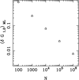
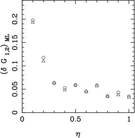
Figure 1: Behaviour of the statistical error $(\delta G_{1})_{ML}$ (circle) and $(\delta G_{2})_{ML}$ (triangle) versus number of homodyne data $N$ (left, notice the scaling $\delta G\propto N^{-0.509}$) and quantum efficiency of homodyne detector (right) in the maximum likelihood estimation of $G_{1}$ and $G_{2}$ in the master equation (1). Parameters (left): $G_{1}=3$, $G_{2}=5$, $\eta=0.6$, $\alpha_{0}=5$, $t=1$. Parameters (right): number of data $N=5\times 10^{3}$, $G_{1}=2$, $G_{2}=1$, $\alpha_{0}=8$, $t=1$.

The robustness of the method to low quantum efficiency $\eta$ is a feature of the maximum-likelihood technique [2, 3]. In the present case, however, it is not surprising [see Fig. (1)], because quantum efficiency itself can be described by master equation (1) [4]. Notice the inverse square root behaviour of the statistical errors versus the number $N$ of data in the sample, according to the central limit theorem.

In conclusion, we applied the maximum-likelihood estimation approach to the characterization of linear active optical media through homodyne detection. The resulting method is efficient and provides a precise determination of the absorption and amplification parameters of the master equation using small homodyne data sample.

This work has been supported by the Italian Ministero dell’Università e della Ricerca Scientifica e Tecnologica (MURST) under the co-sponsored project 1999 Quantum Information Transmission And Processing: Quantum Teleportation And Error Correction. 1

References

- [1] L. Mandel and E. Wolf, Optical Coherence and Quantum Optics, (Cambridge Univ. Press, 1995).
- [2] K. Banaszek, G. M. D’Ariano, M. G. A. Paris, and M. F. Sacchi, Phys. Rev. A 61 10304(R) (2000).
- [3] G. M. D’Ariano, M. G. A. Paris, and M. F. Sacchi, Phys. Rev. A 62 023815 (2000).
- [4] G. M. D’Ariano, C. Macchiavello, and N. A. Sterpi, Quantum Semiclass. Opt. 9, 929 (1997).