On the Number of Elements Needed in a POVM Attaining the Accessible Information

Abstract

We investigate an symmetric set of three quantum states in three dimensions with interesting properties, which we call the lifted trine states. We show that for the ensemble consisting of the three lifted trine states taken with equal probabilities, the POVM measurement realizing the accessible information must contain six projectors, giving a counter-example to a conjecture of Levitin.

Keywords: Quantum measurement; Accessible information; POVM’s

Accessible information was one of the first information-theoretic quantities investigated with respect to quantum systems. The accessible information of an ensemble of quantum states is the maximum mutual information obtainable between the states of the ensemble and the outcomes of a POVM (positive operator valued measurement) on these states. In this paper, we investigate how complicated a measurement which achieves the accessible information must be. Davies’ theorem gives a maximum on the number of elements of the POVM needed to attain the accessible information; namely, if the ensemble being considered is contained in a $d$-dimensional Hilbert space, then at most $d^{2}$ elements are needed in an optimal POVM. When all the states are real, this bound can be improved to $d(d-1)/2$ [7]. C. Fuchs and A. Peres [2] have done numerical studies on ensembles containing only two elements. They found no examples where more than $d$ states were needed; that is, they found that the optimal measurement could always be a von Neumann measurement. In two dimensions, this was proved by Levitin [5], who also conjectured that in $d$ dimensions, if the number of quantum states in the ensemble is at most $d$, a von Neumann measurement is sufficient to attain the accessible information. In this paper, we give an ensemble of three real quantum states in three dimensions, where a POVM attaining the accessible information must contain at least six elements, the maximum by Davies’ theorem.

We investigate the accessible information of an ensemble consisting of three quantum states we call the lifted trine states, with equal probabilities on these states. The lifted trine states are obtained by starting with the two-dimensional quantum trine states: $(1,0)$, $(-1/2,\sqrt{3}/2)$, $(-1/2,-\sqrt{3}/2)$, introduced by Holevo [3] and later studied by Peres and Wootters [6]. We add a third dimension to the Hilbert space of the trine states, and lift all of the trine states out the plane into this dimension by an angle of $\arcsin\sqrt{\alpha}$, so the states become $(\sqrt{1-\alpha},0,\sqrt{\alpha})$, and so forth. We will be dealing with small $\alpha$ (roughly, $\alpha<.1$), so that they are close to being planar. This is the most interesting regime. When the trine states are lifted further out of the plane, they start behaving in relatively uninteresting ways until they are close to being vertical; then they start being interesting again, but this second regime is beyond the scope of this paper. The lifted trine states are thus:

$$T_{0}(\alpha) = (\sqrt{1-\alpha},0,\sqrt{\alpha})$$

$$T_{1}(\alpha) = (-{\textstyle{\frac{1}{2}}}\sqrt{1-\alpha},{\textstyle{\frac{\sqrt{3}}{2}}}\sqrt{1-\alpha},\sqrt{\alpha})$$ (1)

$$T_{2}(\alpha) = (-{\textstyle{\frac{1}{2}}}\sqrt{1-\alpha},-{\textstyle{\frac{\sqrt{3}}{2}}}\sqrt{1-\alpha},\sqrt{\alpha})$$

When it is clear what $\alpha$ is, we may drop it from the notation and use $T_{0}$, $T_{1}$, and $T_{2}$.

In this section, we find the accessible information for this ensemble of lifted trine states. The accessible information is defined as the maximal mutual information between the trine states (with probabilities $\frac{1}{3}$ each) and the elements of a POVM measuring these states. Because the lifted trine states are real vectors, it follows from the version of Davies’ theorem for real states [7] that there is an optimal POVM with at most six elements, all the components of which are real. The lifted trine states are three-fold symmetric, so by symmetrizing we can assume that the optimal POVM is three-fold symmetric (possibly at the cost of introducing extra POVM elements). Also, the optimal POVM can be taken to have one-dimensional elements $E$, so the elements can be described as vectors $\left|\,v_{i}\right\rangle$ where $E_{i}=\left|\,v_{i}\right\rangle\left\langle v_{i}\,\right|$. This means that there is an optimal POVM whose vectors come in triples of the form: $\sqrt{p}P_{0}(\phi,\theta)$, $\sqrt{p}P_{1}(\phi,\theta)$, $\sqrt{p}P_{2}(\phi,\theta)$, where $p$ is a scalar probability and

$$P_{0}(\phi,\theta) = (\cos\phi\cos\theta,\cos\phi\sin\theta,\sin\phi)$$

$$P_{1}(\phi,\theta) = (\cos\phi\cos(\theta+2\pi/3),\cos\phi\sin(\theta+2\pi/3),\sin\phi)$$ (2)

$$P_{2}(\phi,\theta) = (\cos\phi\cos(\theta-2\pi/3),\cos\phi\sin(\theta-2\pi/3),\sin\phi).$$

Suppose that the optimal POVM has several such triples, which we call $\sqrt{p_{1}}\,P_{b}(\phi_{1},\theta_{1})$, $\sqrt{p_{2}}\,P_{b}(\phi_{2},\theta_{2})$, $\ldots$, $\sqrt{p_{m}}\,P_{b}(\phi_{m},\theta_{m})$. It is easily seen that the conditions for this set of vectors to be a POVM are that

$$\sum_{i=1}^{m}p_{i}\sin^{2}(\phi_{i})=1/3{\mathrm{\quad and\quad}}\sum_{i=1}^{m}p_{i}=1.$$ (3)

The formula for accessible information $I_{A}$ can be broken into pieces so that each triple contributes a linear amount to $I_{A}$. That is, $I_{A}$ is the weighted average (weighted according to $p_{i}$) of some contribution $I(\phi,\theta)$ from each $(\phi,\theta)$. To show this, recall that $I_{A}$ is the mutual information between the input and the output, and this can be expressed as the entropy of the input less the entropy of the input given the output, $H(X_{\mathrm{in}})-H(X_{\mathrm{in}}|X_{\mathrm{out}})$. The term $H(X_{\mathrm{in}}|X_{\mathrm{out}})$ naturally decomposes into terms corresponding to the various POVM outcomes, and there are several ways of assigning the entropy of the input $H(X_{\mathrm{in}})$ to the various POVM elements in order to complete this decomposition. Following this analysis eventually gives the same answer as is obtained below (and is in fact how I arrived at it). I briefly sketch this analysis so as to give the intuition behind it, and then go into detail in a second analysis, which is superior in that it explains the form of the answer.

For each $\phi$, and each $\alpha$, there is a $\theta$ that optimizes $I(\phi,\theta)$. This $\theta$ starts out at $\pi/6$ for $\phi=0$, decreases until it hits 0 at some value of $\phi$ (which depends on $\alpha$), and stays at $0$ until $\phi$ reaches its maximum value of $\pi/2$. For a fixed $\alpha$, by finding (numerically) the optimal value of $\theta$ for each $\phi$ and using it to obtain the contribution to $I_{A}$ attributable to that $\phi$, we get a curve giving the optimal contribution to $I_{A}$ for each $\phi$. If this curve is plotted, with the $x$-value being $\sin^{2}\phi$ and the $y$-value being the contribution to $I_{A}$, an optimal POVM is obtained from the set of points on this curve whose average $x$-value is $1/3$ (from Eq. 3), and whose average $y$-value is as large as possible given this constraint on the $x$-values. A simple convexity argument shows that we only need at most two points from the curve to obtain this optimum, and that we will need one or two points depending on whether the relevant part of the curve is concave or convex. For small $\alpha$, it turns out that the relevant piece of the curve is convex, and we need two $\phi$’s to achieve the maximum. Each of these $\phi$’s corresponds to a triple of POVM elements. One of the $(\phi,\theta)$ pairs is $(0,\pi/6)$, and the other is $(\phi_{\alpha},0)$ for some $\phi_{\alpha}>\arcsin(1/\sqrt{3})$. The formula for this $\phi_{\alpha}$ will be derived later.

The analysis in the remainder of this section shows that this six-outcome optimal POVM can be described in a different way, which unifies the optimal measurements for the different $\alpha$’s. For small $\alpha$ ($\alpha<\gamma_{1}$ for some constant $\gamma_{1}$), we first take the trine $T_{b}(\alpha)$ and make a partial measurement which either projects it down to the $x,y$ plane or lifts it further out of the plane so that it becomes the trine $T_{b}(\gamma_{1})$. (Note that $\gamma_{1}$ is independent of $\alpha$.) If the trine was projected into the $x,y$ plane, we make a second measurement using the POVM with outcome vectors $\sqrt{2/3}(0,1)$ and $\sqrt{2/3}(\pm\sqrt{3}/2,-1/2)$. This is the optimal POVM for trines in the $x,y$-plane. If the trine was lifted up, we use the von Neumann measurement that projects onto the basis containing $(\sqrt{2/3},0,\sqrt{1/3})$ and $(-\sqrt{1/6},\pm\sqrt{1/2},\sqrt{1/3})$. If $\alpha$ is larger than $\gamma_{1}$ (but still smaller than $8/9$) we skip the first partial measurement, and just use the above von Neumann measurement. Here, $\gamma_{1}$ is obtained by numerically solving a fairly complicated equation; we suspect that no closed form expression for $\gamma_{1}$ exists. The value of $\gamma_{1}$ is .061367, which is $\sin^{2}\phi$ for $\phi=.25033$ radians ($14.343^{\circ}$).

We now give more details on this decomposition of the POVM into a two-step process. We first apply a partial measurement which does not extract all of the quantum information, i.e., it leaves a quantum residual state that is not completely determined by the measurement outcome. Formally, we apply one of a set of matrices $A_{i}$ satisfying $\sum_{i}A_{i}^{\dagger}A_{i}=I$. If we start with a pure state $\left|\,v\right\rangle$, we observe the $i$’th outcome with probability $\left\langle v\,\right|A_{i}^{\dagger}A_{i}\left|\,v\right\rangle$, and in this case the state $\left|\,v\right\rangle$ is taken to the state $A_{i}\left|\,v\right\rangle$. For our purposes, we choose as the $A_{i}$’s the matrices $\sqrt{p_{i}}\,M(\phi_{i})$ where

$$M(\phi)=\left(\begin{array}[]{ccc}\sqrt{\frac{3}{2}}\cos\phi&0&0\\ 0&\sqrt{\frac{3}{2}}\cos\phi&0\\ 0&0&\sqrt{3}\sin\phi\end{array}\right)$$ (4)

The $\sqrt{p_{i}}\,M(\phi_{i})$ will form a valid partial measurement if and only if $\sum_{i}p_{i}\sin^{2}(\phi_{i})$ $=$ $1/3$ and $\sum_{i}p_{i}=1$, the same conditions [Eq. (3)] as for the $P_{b}(\phi_{i},\theta_{i})$. By first applying the above $\sqrt{p_{i}}\,M(\phi_{i})$, and then applying the von Neumann measurement with the three basis vectors

$$V_{0}(\theta) = \textstyle\Big{(}\sqrt{\frac{2}{3}}\cos(\theta),\sqrt{\frac{2}{3}}\sin(\theta),\frac{1}{\sqrt{3}}\Big{)}$$

$$V_{1}(\theta) = \textstyle\Big{(}\sqrt{\frac{2}{3}}\cos(\theta+2\pi/3),\sqrt{\frac{2}{3}}\sin(\theta+2\pi/3),\frac{1}{\sqrt{3}}\Big{)}$$ (5)

$$V_{2}(\theta) = \textstyle\Big{(}\sqrt{\frac{2}{3}}\cos(\theta-2\pi/3),\sqrt{\frac{2}{3}}\sin(\theta-2\pi/3),\frac{1}{\sqrt{3}}\Big{)}$$

we obtain the POVM given by the vectors $\sqrt{p_{i}}\,P_{b}(\theta_{i},\phi_{i})$; checking this is simply a matter of verifying that $V_{b}(\theta)M(\phi)=P_{b}(\theta,\phi)$. Now, after applying $\sqrt{p_{i}}\,M(\phi_{i})$ to the trine $T_{0}(\alpha)$, we get the vector

$$\big{(}\sqrt{3/2}\sqrt{1-\alpha}\sqrt{p_{i}}\cos\phi_{i},0,\sqrt{3}\sqrt{\alpha}\sqrt{p_{i}}\sin\phi_{i}\big{)}.$$ (6)

This is just the state $\sqrt{p_{i}^{\prime}}\,T_{0}(\alpha_{i}^{\prime})$ where $T_{0}(\alpha_{i}^{\prime})$ is the trine state with

$$\alpha_{i}^{\prime}=\frac{\alpha\sin^{2}\phi_{i}}{\alpha\sin^{2}\phi_{i}+\frac{1}{2}(1-\alpha)\cos^{2}\phi_{i}}$$ (7)

and

$$p_{i}^{\prime}=3p_{i}\left[\alpha\sin^{2}\phi+{\textstyle{\frac{1}{2}}}(1-\alpha)\cos^{2}\phi\right]$$ (8)

is the probability that we observe this trine state, given that we started with $T_{0}(\alpha)$. Similar formulae hold for the trine states $T_{1}$ and $T_{2}$. We compute that

$$\sum_{i}p_{i}^{\prime}\alpha_{i}^{\prime}=\sum_{i}3p_{i}\alpha\sin^{2}(\phi_{i})=\alpha.$$ (9)

Also notice that the first stage of this process, the partial measurement which applies the matrices $\sqrt{p_{i}}\,M(\phi_{i})$, reveals no information about which of $T_{0}$, $T_{1}$, $T_{2}$ that we started with. Thus, by the chain rule for classical Shannon information [1], the accessible information obtained by our two-stage measurement is just the weighted average (the weights being $p^{\prime}_{i}$) of the maximum over $\theta$ of the Shannon mutual information $I_{\alpha_{i}^{\prime}}(\theta)$ between the outcome of the von Neumann measurement $V(\theta)$ and the trines $T(\alpha_{i}^{\prime})$. By convexity, it suffices to use only two values of $\alpha_{i}^{\prime}$ to obtain this maximum. In fact, the optimum is obtained using either one or two values of $\alpha_{i}^{\prime}$ depending on whether the function

$$I_{\alpha^{\prime}}=\max_{\theta}I_{\alpha^{\prime}}(\theta)$$

is concave or convex over the appropriate region. In the remainder of this section, we give the results of computing (numerically) the values of this function $I_{\alpha^{\prime}}$, and we show that for small enough $\alpha$ it is convex, so that we need two values of $\alpha^{\prime}$. We will then show that obtaining this maximum requires a POVM with six outcomes.

Figure 1: The value of $\theta$ maximizing $I_{\alpha}$ for $\alpha$ between $0$ and $.07$. This function starts at $\pi/6$ at $\alpha=0$, decreases until it hits $0$ at $\alpha=.056651$ and stays at $0$ for larger $\alpha$.

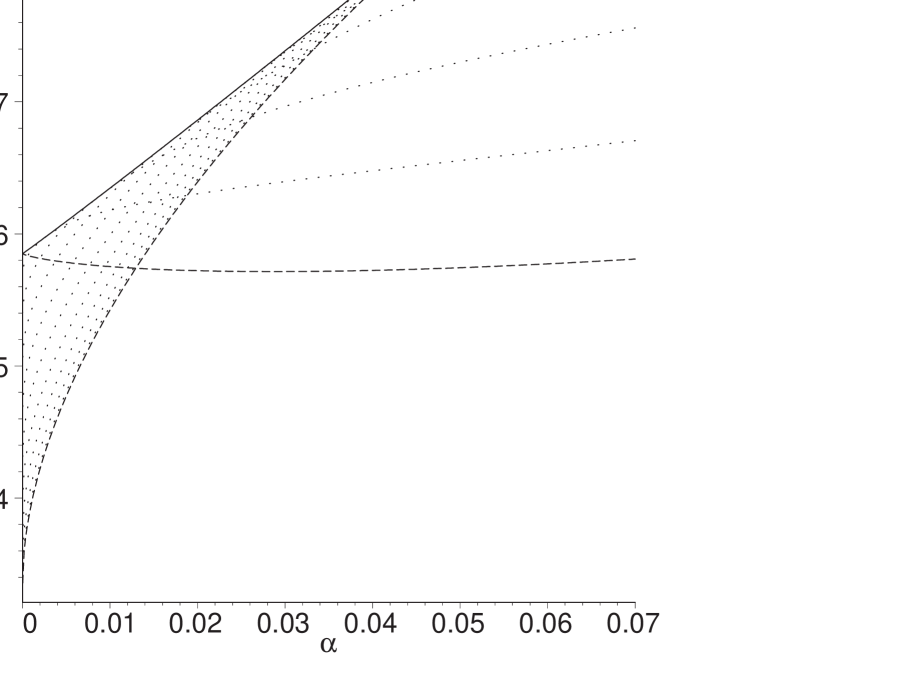
Figure 2: This plot shows $I_{\alpha}(\theta)$ for various $\theta$. The dashed curves are $I_{\alpha}(0)$ and $I_{\alpha}(\pi/6)$. Note that $\theta=0$ is optimal for $\alpha>.056651$ and $\theta=\pi/6$ is optimal for $\alpha=0$. The dotted curves show $I_{\alpha}(\theta)$ for $\theta$ at intervals of $3^{\circ}$ between $0$ and $\pi/6=30^{\circ}$. The solid curve shows $I_{\alpha}(\theta_{\rm opt})$ for those $\alpha$ where neither $0$ nor $\pi/6$ is the optimal $\theta$. The solid curve is slightly convex; this is clearer in Fig. 3.

We need to calculate the Shannon capacity of the channel whose input is one of the three trine states $T(\alpha^{\prime})$, and whose output is determined by the von Neumann measurement $V(\theta)$. Because of the symmetry, we can calculate this using only the first projector $V_{0}$. The Shannon mutual information between the input and the output is $H(X_{\mathrm{in}})-H(X_{\mathrm{in}}|X_{\mathrm{out}})$, which is

$$I_{\alpha^{\prime}}=\log_{2}3+\sum_{b=0}^{2}\langle V_{0}(\theta)|T_{b}(\alpha^{\prime})\rangle^{2}\log\left(\langle V_{0}(\theta)|T_{b}(\alpha^{\prime})\rangle^{2}\right).$$ (10)

We compute that the $\theta$ giving the maximum $I_{\alpha}^{\prime}$ is $\pi/6$ when $\alpha^{\prime}=0$, decreases continuously to 0 at $\alpha^{\prime}=.056651$ and remains 0 for larger $\alpha^{\prime}$. (See Fig. 1.) This value $.056651$ corresponds to an angle of .24032 radians ($13.769^{\circ}$). This $\theta$ was determined by using the computer package Maple to numerically find the point at which $dI_{\alpha}(\theta)/d\theta=0$.

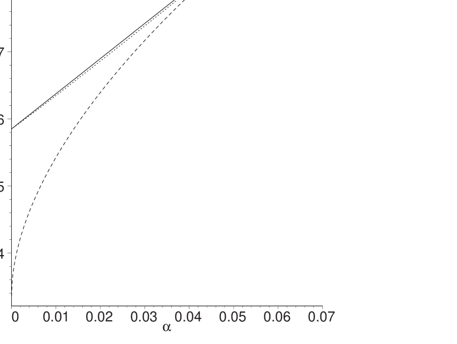
Figure 3: This graph contains three curves. The dashed curve is $I_{\alpha}(0)$ and the dotted curve is the maximum over $\theta$ of $I_{\alpha}(\theta)$ for $\alpha<.056651$. The solid curve is the convex envelope of the other two curves. This solid curve is a linear interpolation between $\alpha=0$ and $\alpha=.061367$ and corresponds to a POVM having six elements. It gives the accessible information for the lifted trine states $T(\alpha)$ when $0\leq\alpha\leq.061367$.

By plugging this optimum $\theta$ into the formula for $I_{\alpha^{\prime}}$, we obtain the optimum von Neumann measurement of the form $V$ above. We believe that this is also the optimal generic von Neumann measurement, but we have not proved this. The maximum of $I_{\alpha^{\prime}}(\theta)$ over $\theta$, and curves that show the behavior of $I_{\alpha^{\prime}}(\theta)$ for constant $\theta$, are plotted in Fig. 2. We can now observe that the first part of the curve is convex, and thus that for small $\alpha$ the best POVM will have six projectors, corresponding to two values of $\alpha^{\prime}$. We calculate that for trine states with $\alpha<.061367$, the two values of $\alpha^{\prime}$ giving the maximum accessible information are $0$ and $.061367$; we will let $\gamma_{1}=.061367$ be this second value. The trine states $T(\gamma_{1})$ make an angle of .25033 radians ($14.343^{\circ}$) with the $x$-$y$ plane. The accessible information thus obtained is plotted in Fig. 3.

We can now invert the formula for $\alpha^{\prime}$ (Eq. 7) to obtain a formula for $\sin^{2}(\phi)$, and substitute the value of $\alpha^{\prime}=\gamma_{1}$ back into the formula to obtain the optimal POVM. We find

$$\sin^{2}(\phi_{\alpha}) = \frac{1-\alpha}{1+\alpha\left(\frac{2-3\gamma_{1}}{\gamma_{1}}\right)}$$ (11)

$$= \frac{1-\alpha}{1+29.591\alpha}$$

where $\gamma_{1}=.061367$ as above. Thus, the elements in the optimal POVM we have found for the trines $T(\alpha)$, when $\alpha<\gamma_{1}$, are the six vectors $P_{b}(\phi_{\alpha},0)$ and $P_{b}(0,\pi/6)$, where $\phi_{\alpha}$ is given by Eq. 11 and $b=0,1,2$. We must also prove there are no other POVM’s which attain the same accessible information. The argument above shows that any optimal POVM must contain only projectors chosen from these six vectors: only those two values of $\alpha^{\prime}$ can give the maximum capacity, and for each of these values of $\alpha^{\prime}$ there are only three projectors in $V(\theta)$ which can maximize $I_{\alpha^{\prime}}$ for these $\alpha^{\prime}$. It is easy to check that there is only one set of probabilities $p_{i}$ which make the above six vectors into a POVM, and that none of these probabilities are 0 for $0<\alpha<\gamma_{1}$. Thus, for the lifted trine states with $0<\alpha<.061367$, there is only one POVM maximizing accessible information, and it contains six elements, the maximum possible for real states by a generalization of Davies’ theorem [7].

References

- [1] T. M. Cover and J. A. Thomas, Elements of Information Theory, Wiley, New York, 1991.
- [2] C. Fuchs, personal communication.
- [3] A. S. Holevo, “Information-theoretical aspects of quantum measurement,” Problemy Peredachi Informatsii vol. 9, no. 2, pp. 31–42 1973 (in Russian); English translation: A. S. Kholevo, Problems of Information Transmission, vol. 9, pp. 110-118, 1973.
- [4] A. S. Holevo, “Coding theorems for quantum channels,” Russian Math Surveys, vol. 53, pp. 1295–1331, 1998; LANL e-print quant-ph/9809023.
- [5] L. B. Levitin, “Optimal quantum measurements for two pure and mixed states,” in Quantum Communications and Measurement (V. P. Belavkin, O. Hirota and R. L. Hudson, eds.), Plenum Press, New York, 1995, pp. 439–448.
- [6] A. Peres and W. K. Wootters, “Optimal Detection of Quantum Information,” Phys. Rev. Lett., vol. 66, pp. 1119–1122 (1991).
- [7] M. Sasaki, S. M. Barnett, R. Jozsa, M. Osaki and O. Hirota, “Accessible information and optimal strategies for real symmetrical quantum sources,” Phys. Rev. A, vol. 59, 3325–3335, 1999, LANL e-print quant-ph/9812062.
- [8] C. E. Shannon, “A mathematical theory of communication,” The Bell System Tech. J., vol. 27, pp. 379–423, 623–656, 1948.