Classical wave-optics analogy of quantum information processing

Abstract

An analogous model system for quantum information processing is discussed, based on classical wave optics. The model system is applied to three examples that involve three qubits: (i) three-particle Greenberger-Horne-Zeilinger entanglement, (ii) quantum teleportation, and (iii) a simple quantum error correction network. It is found that the model system can successfully simulate most features of entanglement, but fails to simulate quantum nonlocality. Investigations of how far the classical simulation can be pushed show that quantum nonlocality is the essential ingredient of a quantum computer, even more so than entanglement. The well known problem of exponential resources required for a classical simulation of a quantum computer, is also linked to the nonlocal nature of entanglement, rather than to the nonfactorizability of the state vector.

03.67.Lx, 03.65.Bz, 42.50.-p, 42.79.Ta

I Introduction

The processing of quantum information is under intense investigation because it enables applications which are either impossible or much less efficient without the use of quantum mechanics [1, 2, 3, 4]. For example, secret keys for encrypted communication can be distributed in ways that do not allow an eavesdropper to gain information about the key [5, 6, 7, 8, 9]. A formidable challenge still remains in the development of a universal quantum computer, which should be able to solve certain problems in a polynomial time where a classical computer requires exponential time.

In this paper we explore an analogy of quantum information processing, based on classical (optical) waves [10, 11, 12]. This approach is inspired by the observation that some of the essential properties of quantum information are in fact wave properties, where the wave need not be a quantum wave. By exploring the limits to where the classical analogy can be pushed, we aim to obtain information about the subtle but profound differences between the quantum system and the classical wave system. In addition, the classical systems may serve as model systems for the corresponding quantum systems, e.g. elucidating the mathematical structure of a problem.

Quantum bits, or “qubits” [13] are different from classical bits in several important ways. A first important difference is that qubits can exist in a superposition of the two binary states $\{|0\rangle,|1\rangle\}$. A second crucial difference is that qubits can be entangled. Superpositions are of course well known for classical waves, so they are not exclusively quantum mechanical. Entanglement, on the other hand, is commonly regarded as a quintessential quantum phenomenon. It typically plays a role whenever quantum physics defies “common sense” and produces counterintuitive effects. Famous examples are Schrödinger’s cat [14, 15, 16], the Einstein-Podolsky-Rosen paradox [17], Bell’s inequality [18, 19], and, more recently, in quantum cryptography [5, 6, 7, 8, 9], teleportation [20, 21, 22, 23] and quantum computation [2, 3].

A classical analogy of entanglement has previously been constructed on the basis of classical (light) waves [10, 11]. The analogy captures most features typically associated with entanglement, such as a nonfactorizable state vector. However, the analogy fails to produce effects of quantum nonlocality, thus signaling a profound difference between two types of entanglement: (i) “true,” multiparticle entanglement and (ii) a weaker form of entanglement between different degrees of freedom of a single particle. Although these two types look deceptively similar in many respects, only type (i) can yield nonlocal correlations. Only the type (ii) entanglement has a classical analogy.

In this paper the analogy is applied to concepts from quantum information processing, such as elementary quantum gates and simple quantum networks. We extend previous work on optical analogies, concentrating here in particular on three-bit examples. We explore how far we can push the classical analogy and to what extent the classical system may be useful.

We start in Sec. II by briefly reviewing the concepts outlined in Ref. [10], introducing the “cebit” as the classical counterpart of the qubit. The next three sections, III–V, are each devoted to one specific application of the classical analogy. In Sec. III three-cebit entanglement, or so-called Greenberger-Horne-Zeilinger states, is discussed. In Sec. IV the teleportation of a cebit is discussed. In Sec. V a simple error correction network is described, which can correct either bit flips or phase errors. Finally, in Sec. VI we discuss how the resources required by the analogy scale with the number of cebits. Conclusions are given in Sec. VII.

II A classical Hilbert space of cebits

We briefly review the classical analogy as described by Spreeuw [10] and which is closely similar to that described by Cerf et al. [11]. The state vector of a qubit, $|\psi\rangle=q_{0}|0\rangle+q_{1}|1\rangle$, is specified by two complex probability amplitudes, $(q_{0},q_{1})$. We replace these by two complex classical wave amplitudes, the argument of the complex amplitudes representing the phase. The resulting two-component complex vector $(c_{0},c_{1})$ is the classical counterpart of a qubit and will be called a cebit. The amplitudes $(c_{0},c_{1})$ may be macroscopic and can in principle be measured directly. It should be noted that the choice of optical waves is not essential for the analogy. Other classical waves such as sound, water waves, or even coupled pendula could be used in principle.

We write the cebits in a notation which is a slightly modified version of the familiar bra-ket notation of quantum mechanics. We use parentheses for the cebits, instead of brackets, so that it is always evident whether we are dealing with cebits or qubits. Similar to the bra and ket pair, we use a parent $(\theta|$ and thesis $|\theta)$, which are Hermitian conjugate to each other,

$$|\theta) = c_{0}|0)+c_{1}|1)$$ (1)

$$(\theta| = c^{\ast}_{0}(0|+c^{\ast}_{1}(1|$$ (2)

The cebits form a Hilbert space where the Hermite product is given by “parentheses,” e.g. $(\theta|\theta)=|c_{0}|^{2}+|c_{1}|^{2}$.

As an example of a cebit, we can take the pair of complex amplitudes describing the horizontal and vertical polarization components of a laser beam. This two-component complex vector is known as a Jones vector [24]. Here we will call it the polarization cebit. Alternatively we can take the complex amplitudes of two spatially separate laser beams (spatial modes). The two amplitudes now being associated with position rather than polarization, we will call this pair a position cebit.

A Measurements and unitary operations on a cebit

Measurements on a cebit can be performed using photodetectors. For the measurement of a polarization cebit we place photodetectors at the outputs of a polarizing beam splitter, which transmits the horizontal and reflects the vertical component, see Fig. 1(a). Identifying the transmitted and reflected components with the amplitudes $c_{0}$ and $c_{1}$, respectively, the photodetector signals are proportional to $|c_{0}|^{2}$ and $|c_{1}|^{2}$.

Instead of the intensities, one could in principle also measure the amplitude and phase of the classical wave. Depending on the frequency, the complex amplitudes could be measured either directly, or by mixing them with a strong local oscillator in a homo- or heterodyne measurement. Here we restrict ourselves to intensity measurements, which also give access to complete information about the complex amplitudes. The reason is that one can first produce two identical copies of a classical light beam using a beam splitter, and perform measurements on the copies in different bases of measurement. With qubits this is of course impossible, since they cannot be copied.

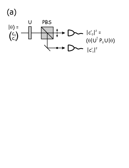
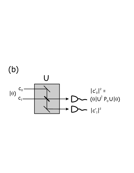
FIG. 1.: (a) Measurement of a polarization cebit $|\theta)$ using a polarizing beamsplitter PBS and photodetectors. The signals are “expectation values” of projection operators, $P_{i}=|i)(i|$. Measurements in a different basis can be performed by first performing a unitary operation $U$ on the polarization. (b) Measurement of a position cebit. In this case the unitary operation consists of a beamsplitter with variable splitting ratio and phase.

A measurement can be performed in a different basis by first performing a unitary operation on the cebit, $|\theta)\rightarrow|\theta^{\prime})=U|\theta)$. Writing $(c^{\prime}_{0},c^{\prime}_{1})$ for the amplitudes of $|\theta^{\prime})$, the measured signals are

$$|c^{\prime}_{i}|^{2}=(\theta^{\prime}|P_{i}|\theta^{\prime})=(\theta|U^{{\dagger}}P_{i}U|\theta),$$ (3)

where $P_{i}=|i)(i|$ are projection operators. For the polarization cebit the transformation $U$ is performed using polarization optics, such as quarter-wave plates (QWP), polarization rotators, etc. For example, a Hadamard gate can be realized by a half-wave plate (HWP), its fast axis oriented at $22.5^{\circ}$ with respect to the vertical direction, see also Fig. 5(a). More general, a universal SU(2) operator can be realized by a sequence of three rotatable retarders, QWP-HWP-QWP [25].

For a measurement on a position cebit we simply place photodetectors in each beam of the beam pair to measure two intensities proportional to $|c_{0}|^{2}$ and $|c_{1}|^{2}$. A different measurement basis can again be obtained by first performing a unitary operation, see Fig. 1(b). This operation should now mix the two spatially separated amplitudes, using beam splitters. The Hadamard gate can be realized by a 50/50 beam splitter, with properly adjusted phases of the inputs and outputs, see Fig. 5(b). A universal SU(2) operator can be realized by a Mach-Zehnder interferometer, consisting of two 50/50 beam splitters and three adjustable phase delays: in one of the inputs, in one of the interferometer arms, and in one of the outputs [26]. In fact it has been shown that any unitary $N\times N$ matrix can be realized as an optical multiport [27].

B Multiple cebits

We can generalize this procedure and construct the Hilbert space of multiple cebits, which should be spanned by the tensor products of basis states of the Hilbert spaces of the individual cebits. We concentrate here on a system of three cebits. Since the quantum state of three qubits is described by eight probability amplitudes,

$$|\Psi\rangle=q_{000}|000\rangle+q_{001}|001\rangle+\ldots+q_{111}|111\rangle,$$ (4)

the corresponding cebit version should also contain eight amplitudes. This can be accomplished using four laser beams with polarization.

We label the amplitudes $c_{000}\ldots c_{111}$ as shown in Fig. 2. Each pair of amplitudes $(c_{ij0},c_{ij1})$ constitutes the Jones polarization vector of one of the four beams. One might thus easily, though wrongly, identify each of the four Jones vectors with one cebit. In fact the four Jones vectors constitute only three cebits. Four amplitudes are associated with any bit value of a given cebit. For example, the subspace where the polarization cebit has value 0 is specified by four amplitudes that vanish, $c_{ij1}=0$.

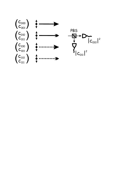
FIG. 2.: Eight classical wave amplitudes of four polarized beams, together encoding three cebits. The first cebit is here depicted by line style (solid for 0, dotted for 1), the second by arrow style (single for 0, double for 1), the third by polarization (vertical for 0, horizontal for 1).

The remaining two cebits are position cebits. The “most significant cebit” (MSC), associated with the first index $i$ of $c_{ijk}$, describes coarse position, bit value 0 meaning that the lower beam pair is dark. The middle bit $j$ describes the fine position, within a pair of beams, bit value 0 now meaning that the lower beam within each beam pair is dark. In Fig. 2 the bit values for the MSC are indicated by line style (solid vs. dashed), for the middle cebit by arrow head style (single vs. double) and for the least significant cebit by polarization direction (arrow vs. dot.)

III Greenberger-Horne-Zeilinger states

As a first example of three-bit states we construct the optical analog of the three-particle entangled state introduced by Greenberger, Horne, and Zeilinger (GHZ) [28, 29],

$$|\Psi_{\rm GHZ}\rangle=\frac{1}{\sqrt{2}}\left(|000\rangle+|111\rangle\right).$$ (5)

Let us first briefly recall the remarkable properties of this quantum state. These become apparent by measuring the four different observables $\sigma_{x}^{2}\sigma_{y}^{1}\sigma_{y}^{0}$, $\sigma_{y}^{2}\sigma_{x}^{1}\sigma_{y}^{0}$, $\sigma_{y}^{2}\sigma_{y}^{1}\sigma_{x}^{0}$, and $\sigma_{x}^{2}\sigma_{x}^{1}\sigma_{x}^{0}$, (in short: “$xyy$”, “$yxy$”, “$yyx$”, and “$xxx$”, respectively). Here, $\sigma_{j}^{i}\,(j=x,y,z)$ are the Pauli matrices for qubit $i$,

$$\sigma_{x}=\left(\begin{array}[]{cc}0&1\\ 1&0\end{array}\right),\,\sigma_{y}=\left(\begin{array}[]{cc}0&-i\\ i&0\end{array}\right),\,\sigma_{z}=\left(\begin{array}[]{cc}1&0\\ 0&-1\end{array}\right)$$ (6)

The first three measurements, on $xyy$, $yxy$, and $yyx$, all yield the value $-1$, since $|\Psi_{\rm GHZ}\rangle$ is an eigenstate with eigenvalue $-1$. We could now attempt to predict the outcome of the fourth measurement, on $xxx$, by assigning values $+1$ or $-1$ to the individual spin components. For example, we could assign $\sigma_{x}^{2}=\sigma_{y}^{1}=\sigma_{x}^{0}=+1$ and $\sigma_{y}^{2}=\sigma_{x}^{1}=\sigma_{y}^{0}=-1$. This would predict a value $-1$ for the $xxx$ measurement. There are eight possible combinations of such assignments, predicting unanimously the value $-1$ for $xxx$. On the other hand, the quantum prediction is $+1$, since $|\Psi_{\rm GHZ}\rangle$ is an eigenstate of $\sigma_{x}^{2}\sigma_{x}^{1}\sigma_{x}^{0}$ with eigenvalue $+1$. The quantum prediction has recently been confirmed experimentally, providing a dramatic demonstration of quantum nonlocality [30, 31].

The optical version, $|\Theta_{\rm GHZ})$, consists of two laser beams with orthogonal polarization (plus two beams which are dark), see Fig. 3. We now pose the obvious question of what will be the outcome of the equivalent cebit measurements for this “classical GHZ state”? We thus have to perform joint measurements on three cebits.

A Joint cebit measurements on the GHZ state

For any three-cebit state $|\theta)$ a measurement on the cebits can be performed by placing polarizing beam splitters (PBS) into each beam plus a photodetector at each output, as shown in Fig. 2. This makes eight photodetectors in total, corresponding to the eight basis states of the three-cebit Hilbert space. The signal of a particular photodetector is proportional to $|c_{ijk}|^{2}$. Note that any given detector is associated with three bit values at once, one for each cebit. The choice of the measurement basis is again done by a unitary operation on the three-cebit state. For example this may consist of a sequence of three unitary operations for each cebit separately, as in Fig. 1.

The GHZ measurement thus translates into a classical interferometer, shown in Fig. 3. It is straightforward to calculate the signals that will be measured at the eight output ports of this interferometer. If we set the measurement basis to $xyy$, we find that four out of eight outputs are dark and that the remaining four have equal intensity. The dark outputs are those labeled by 000, 011, 101, and 110. The remaining, bright, outputs are just the ones corresponding to a measurement result $-1$, if we identify bit values 0 and 1 by spin values $+1$ and $-1$, respectively.

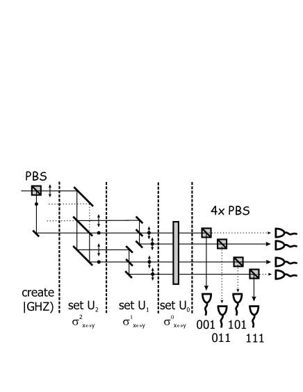
FIG. 3.: Interferometer representing measurements on a three-cebit entangled “GHZ” state. For each cebit $i$, the unitary operation $U_{i}$ sets the measurement basis to $x$ or $y$ (in spin-1/2 space). For $U_{1,2}$ this is done by adjusting the phases of the mirrors and beam splitters. For $U_{0}$ the polarization element is switched between a $45^{\circ}$ rotator ($x$ basis) and a quarter-wave plate oriented at $45^{\circ}$ ($y$ basis). The solid and dashed lines identify the bright and dark outputs for either of the settings $xyy$, $yxy$, or $yyx$. For the setting $xxx$ the bright ports become dark and vice versa. Note that the $U_{i}$ commute, so their order is arbitrary.

The fact that four outputs carry equal intensity shows that the GHZ state is not an eigenstate of any individual cebit operator. Instead, it is an eigenstate of the three-cebit observable $xyy$. In other words, we have not obtained a definite value for any cebit, but instead found that the three cebits are correlated. If we change the measurement basis to $yxy$ or $yyx$, we find that the same four outputs are dark and the same four are bright. So again the measurement result is $-1$, as formulated in GHZ language. The fact that each of the three measurements yields four dark and four bright outputs is a striking demonstration of the failure of any attempts to assign definite values $+1$ or $-1$ to the individual cebit components.

Finally, we change the measurement basis to $xxx$ and find that in this case the four dark outputs have now become the bright ones and vice versa. Apparently the measurement result is now $+1$, in complete correspondence with the quantum result for the real GHZ experiment.

B Discussion

The cebit version of the GHZ experiment thus shows that in general it is impossible to assign definite values to different degrees of freedom of a single particle. The cebit analogy is described by the same mathematics and may thus be used to elucidate the mathematical structure of the problem. On the other hand, the underlying physics is different in a very subtle way.

The measurements on different degrees of freedom (cebits) of a single particle are correlated, but the correlations will never be of a nonlocal nature. The three cebits are by construction always chained together. It is impossible to spatially separate them and perform separate measurements on the three cebits in different locations. Therefore no statements about local realism can be made on the basis of the cebit experiment.

Since the three-cebit GHZ state is a classical state of light, it would of course be possible to make three identical copies and send these to different locations to be analyzed. For example, one could measure $\sigma_{x}^{2}$ in location 2, $\sigma_{y}^{1}$ in location 1, and $\sigma_{y}^{0}$ in location 0. However there will be no correlations between the measurements in different locations. The correlations exist only between the degrees of freedom of each local copy, not between different copies.

Nevertheless it is remarkable that the classical analogy reproduces exactly the quantum correlations, since in the quantum case the nonlocal correlations are commonly associated with the collapse of the wavefunction due to a measurement. In the classical case, the correlations are due to classical wave interference. A choice of measurement basis leads to destructive interference in some output channels, which then appears as correlations of cebit values.

Finally, it should be noted that this GHZ experiment with cebits has not actually been performed experimentally. However, we have described essentially an interferometer for classical light, so there is no reason to doubt these predictions.

IV Teleportation of a cebit

A Teleportation of a qubit

Quantum teleportation allows the transmission of the quantum state of a qubit between a sender and a receiver, usually called Alice and Bob. Alice destroys the qubit by making a measurement, gaining however no information on the qubit. The result of the measurement enables Bob to recreate the qubit. We follow here the concept as introduced by Bennett et al. [20], which has recently been realized experimentally by Bouwmeester et al. [21]. Alternative teleportation schemes have also been demonstrated [22, 23]. The Rome experiment [22] may in fact be considered as a hybrid version, using in addition to the entanglement between two separate photons, also the different degrees of freedom of one photon. For a detailed comparison between the different teleportation schemes, see Ref. [4]. Briefly, the Bennett procedure works as follows.

First Alice and Bob share an EPR pair of qubits, in the entangled state $|\Psi_{\rm EPR}\rangle=(|01\rangle-|10\rangle)/\sqrt{2}$. Alice now performs a Bell state measurement on her part of the EPR pair plus the qubit whose state $|\psi\rangle$ she wants to teleport. This means she performs a measurement on the two-qubit state in the basis of the four Bell states:

$$|\Psi^{\pm}\rangle = \frac{1}{\sqrt{2}}\left(|01\rangle\pm|10\rangle\right)$$ (7)

$$|\Phi^{\pm}\rangle = \frac{1}{\sqrt{2}}\left(|00\rangle\pm|11\rangle\right)$$ (8)

Alice then informs Bob which of the four Bell states she found, by sending him two bits of classical information. Finally, Bob performs one out of four unitary operations on his half of the EPR pair, following the two-bit instruction received from Alice. This leaves Bob’s qubit in the state $|\psi\rangle$.

B Optical implementation

The optical analogy of this protocol is sketched in Fig. 4. A somewhat different implementation has been described in Ref. [11]. The implementation discussed here starts by generating the “EPR pair,” a two-cebit state $|\Theta_{\rm EPR})=[|01)-|10)]/\sqrt{2}$ of entangled position and polarization. This is done using a polarizing beam splitter. In the next step an additional position cebit $|\theta_{2})$ is created. This is the cebit that is to be “teleported”. This additional cebit is created by splitting the EPR pair into two copies with relative amplitudes $c_{0}$ and $c_{1}$. This is done using a Mach-Zehnder interferometer consisting of two 50/50 beam splitters and two adjustable phase delays, $\phi_{1}$ in one of the arms and $\phi_{2}$ in one of the output ports. The to-be-teleported cebit, $|\theta_{2})=c_{0}|0)+c_{1}|1)$, apart from an overall phase, is selected by setting the two phase delays $\phi_{1,2}$.

If we want to teleport position cebit $|\theta_{2})$ into the polarization cebit, we must now perform a Bell state analysis on the two position cebits. In fact it is not necessary to do any photodetection. It is sufficient to perform a basis transformation to the Bell basis, using a set of beam splitters. These mix the $00$ with the $11$ amplitudes and the $01$ with the $10$ amplitudes. After this unitary transformation, the four beams correspond to the four Bell states, i.e. the four possible outcomes of Alice’s measurements.

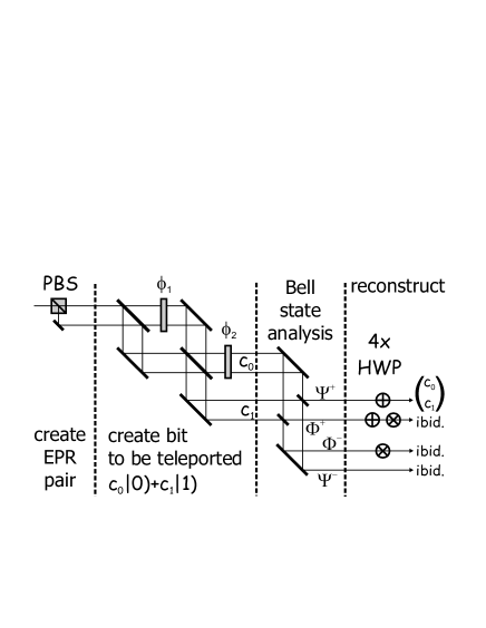
FIG. 4.: Optical network to “teleport” a position cebit to the polarization cebit. In the final state all four beams have the same polarization, with coefficients $(c_{0},c_{1})$ equal to that of the position cebit created earlier.

Finally, depending on the Bell state, one out of four operations is performed on the polarization cebit. This means that a different polarization operation is performed on each of the four beams. The operations are the identity and three different spin rotations by $\pi/2$ about the axes $x$, $y$, and $z$. The optical implementations for the three rotations are respectively: a QWP with its axes rotated by $\pi/4$, a $\pi/2$ optical rotator, and a QWP with its fast axis in the vertical direction. Note that in Fig. 4 the rotator has been replaced by two HWP’s with a relative orientation of $45^{\circ}$.

This optical system teleports the position cebit $|\theta_{2})$ into the polarization cebit. This means that now the four beams carry equal polarization, for every possible setting of the phase delays $\phi_{1,2}$ of the Mach-Zehnder interferometer. Furthermore the polarization is given by the Jones vector $(c_{0},c_{1})$, as determined by the phase delays.

C Discussion

By transforming to the Bell basis and post-processing the polarization, the three-cebit state $[c_{0}|0)+c_{1}|1)]\otimes|\Theta_{\rm EPR})$ has been transformed into the three-cebit state $|\theta_{21})\otimes[c_{0}|0)+c_{1}|1)]$. Here we denote by $|\theta_{21})$ the final state of the two position cebits, 2 and 1. If desired, the two position cebits contained in $|\theta_{21})$ can now be discarded. The four beams have well defined phase relationships, which do not depend on $(c_{0},c_{1})$. Therefore the four beams can be combined into a single beam using beam splitters.

In the end, what we have accomplished is to combine the amplitudes of two different beams into the polarization components of a single beam. Of course, this is a rather trivial optical task that could have been accomplished in a much simpler way. However, by following the teleportation protocol, several subtle differences become clear between qubits and cebits.

In the quantum version, the Bell state analysis seems impossible without a nonlinear process, i.e. interaction between the qubits [32]. In contrast, in the cebit version, the Bell state analysis is easily performed using passive linear components. Again, like in the GHZ example, the inseparability of the cebits in space poses a limitation. Rather than teleporting a qubit state over some distance in space, the state of one cebit is transferred to another cebit. In this case a position cebit was “teleported” to the polarization cebit. However, the source and target cebits are necessarily always part of the same composite multiple-beam system. Bob’s half of the EPR pair and Alice’s classical information cannot be transmitted separately.

V Error correction networks

As a third application of the optical analogy of qubits, we consider a simple error correction network [33, 34], correcting either for bit flip errors or phase errors. In principle, a network that corrects both bit flips and phase flips may also be constructed optically. However, this would require at least five cebits [35, 36], i.e. 16 beams of polarized light. A quantum logic network that corrects bit flips is shown in Fig. 6(a). The correction network for phase errors is obtained by applying a Hadamard gate to each qubit, both before and after the bit flip region. The network makes use of controlled NOT (c-NOT) gates and a Toffoli gate. These are described first.

A Controlled NOT and Toffoli gates

The c-NOT gate for cebits takes several shapes, depending on which cebit is the control bit and which the target. For simplicity, we describe here the c-NOT gates for the situation of two cebits, one position and one polarization cebit.

The simplest situation occurs when the position is the control cebit and the polarization the target. The gate should thus flip the polarization if the position cebit has the value 1, i.e. if the light is in the lower beam. The polarization flip between horizontal and vertical is obtained using a HWP oriented at $45^{\circ}$ with respect to vertical. We simply place the HWP in the lower beam to obtain a c-NOT gate, see Fig. 5(c).

By a simple extension a Toffoli gate is obtained, where both control cebits are position cebits, the target polarization. In this case we have four beams and the subspace where both position cebits have value 1 is formed by the lowermost beam of the four. Therefore the Toffoli gate is implemented by placing the half-wave plate in the lower beam, see Fig. 5(e).

If the roles of target and control bits in the c-NOT gate are reversed, polarization becoming the control and position the target bit, the c-NOT gate becomes somewhat more complicated. Conditioned on the polarization, the gate should reverse the upper and lower beams. This can be accomplished using the optical arrangement shown in Fig. 5(d).

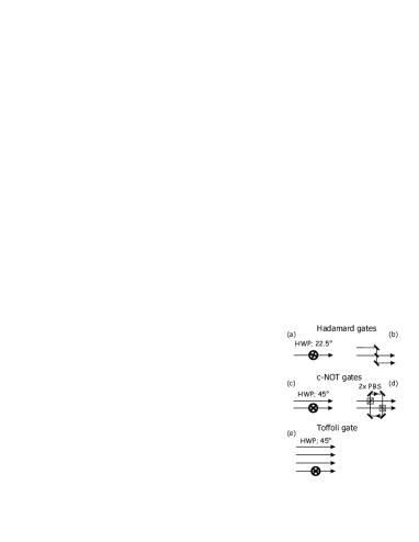
FIG. 5.: Examples of elementary gates for cebits. (a) Hadamard gate for a polarization cebit, consisting of a HWP oriented at $22.5^{\circ}$. (b) Hadamard gate for a position cebit, consisting of a 50/50 beamsplitter. (c) c-NOT gate where the position cebit is the control, the polarization the target. The polarization bit is flipped by means of a half-wave plate (HWP). (d) c-NOT gate, polarization controls position. Polarizing beam splitters (PBS) reroute the beams in such a way that the two beams exchange position, conditioned on the polarization. (e) Toffoli gate, flipping the polarization cebit, conditioned on two position cebits.

B Cebit-flip error correction network

The optical cebit version of the bit-flip correction network is shown in Fig. 6(b). In the qubit version, Fig. 6(a), the first two c-NOT gates serve to store a single qubit into a three-cebit entangled state: $q_{0}|0\rangle+q_{1}|1\rangle\rightarrow q_{0}|000\rangle+q_{1}|111\rangle$.

In the optical cebit version this can be accomplished using a single polarizing beam splitter (PBS), acting on the incident polarization cebit $c_{0}|0)+c_{1}|1)$. The component $c_{1}|1)$ is split off and moved into the fourth beam, whereas the component $c_{0}|0)$ forms the first beam. Thus we obtain the three-cebit state $c_{0}|000)+c_{1}|111)$. The next section in the optical diagram is the region where possible bit flips can occur. The bit flip is corrected using two c-NOT gates and a Toffoli gate. The c-NOT gates are a generalized version of those shown in Fig. 5(d). Both have the polarization as the control cebit and a position cebit as the target. Finally, the Toffoli gate is formed by placing a half-wave plate in the fourth beam, just as in Fig. 5(e).

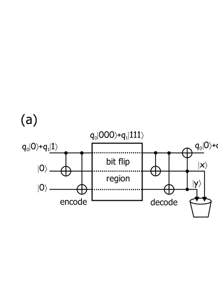
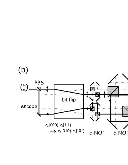
FIG. 6.: (a) Quantum logic network correcting for bit flip errors. (b) The cebit version. The incident polarization is restored and comes out in one of the four output beams, depending on which cebit was flipped. The solid line traces the optical beam path in the case that the middle cebit is flipped. Note that networks correcting for phase errors may be obtained by applying a Hadamard gate on each qubit/cebit, both before and after the bit flip region.

Let us now suppose that the middle cebit flips,

$$c_{0}|000)+c_{1}|111)\rightarrow c_{0}|010)+c_{1}|101).$$ (9)

Optically, this bit flip entails swapping the beams within each pair, i.e. swapping beams 1 and 2 and likewise beams 3 and 4, see Fig. 6(b). In the same Figure we also see how the network corrects the error, by tracing the optical path through the sequence of polarizing beam splitters. Eventually, the two components are recombined so that the original input polarization $c_{0}|0)+c_{1}|1)$ is restored. The port where this restored polarization exits (i.e. the values of the two position cebits) is determined by which cebit was erroneously flipped.

Just like in the qubit version, the entire three-bit state at the output of the error-correction network is uncertain. However, unlike in the qubit version, the two cebits whose state is uncertain cannot easily be discarded. Whereas in the qubit version the two unused bits are separate particles and can be removed, this is no longer possible in the cebit version. Removing the two uncertain cebits would mean recombining the four beams into one. This cannot be done without loss of intensity, because the relative phases and amplitudes are uncertain. The fact that we cannot discard the two unknown cebits can be seen as another failure to simulate the nonlocality in the quantum system. Again this feature is lost in the translation to the cebit version.

VI Scaling and resources

The optical analogy discussed in this paper is based on replacing $n$ two-state particles by a single particle (photon) with $n$ two-state degrees of freedom. Since in both cases we deal with a $2^{n}$-dimensional Hilbert space, the two situations may seem rather similar. However the difference is profound. It is well known that for this simulation procedure one pays the price of exponential resources [1, 37]. Here, each extra cebit doubles the required number of light beams. The amount of optical hardware required also grows exponentially with the number of cebits.

This difference in scaling behavior poses more than merely a technical problem. One can easily see that this is in fact a dramatic limitation by examining how far the classical system could be scaled up. We can attempt to stack light beams as densely as possible. The cross section of a single beam is limited by optical diffraction to the order of the square of the wavelength, or $\lambda^{2}\sim 10^{-12}$ m² in the optical region. In a stretch of the imagination, let us assume that the stack of beams can be made to fill the entire universe, with a diameter $D\sim 10^{26}$ m. The number of beams can then be increased to approximately $(D/\lambda)^{2}\sim 10^{64}$. Although this is a huge number, the number of cebits (using two polarizations) is still only $n=1+\log_{2}10^{64}\approx 214$. Even if we use a wavelength $\lambda\sim 10^{-10}$ m, the number of cebits is no larger than 240.

Another resource that may pose a limitation is the total optical power. Since the light is distributed over an exponentially growing number of light beams, the intensity per beam decreases exponentially. This becomes important if one is interested to eavesdrop on the information processing, i.e. if one wishes to measure the intermediate state. This possibility should in principle exist in a classical system. However, as a result of the exponential scaling behavior the possibility to eavesdrop on the classical system is lost.

Thus the most important difference between qubits and cebits becomes clear by looking at the scaling behavior while increasing the number of bits. Obviously, the amount of required resources like beam splitters and such will also increase exponentially and quickly deplete the available matter in the known universe.

VII Conclusion

In summary, the optical analogy of quantum information, as introduced in Ref. [10] has been applied to three examples involving three qubits/cebits.

The three-cebit “GHZ” entangled state shows that it is impossible to assign values $\pm 1$ to the $x$ and $y$ component of all three cebits, in such a way that all joint measurements are correctly predicted. The predicted results are formally identical to the quantum predictions for the qubit version of the experiment. Thus the optical analogy is a useful tool to visualize and elucidate the mathematical structure of the problem. The crucial difference is that the three cebits cannot be spatially separated, so that the optical system cannot be used for testing local realism.

Like in the GHZ example, in the example of teleportation the unseparability of the cebits in space again poses a limitation. Rather than teleporting a qubit state over a distance in space, the state of one cebit is transferred to another cebit. In the example, a position cebit was “teleported” to the polarization cebit. However, the source and target cebits are always part of the same composite multiple-beam system.

In the third example we considered a simple error correction network that corrects for either bit flips or phase errors. The limitation encountered here was that the extra two cebits required for the correction network cannot be easily disposed of after finishing the protocol. This limitation can again be seen as a consequence of the lack of nonlocality.

The analogy is based on replacing the $2^{n}$-dimensional Hilbert space of $n$ two-state particles (qubits) by the $2^{n}$-dimensional Hilbert space of a single particle (photon) with $n$ two-state degrees of freedom. It is well known that by doing so, one pays the price of exponential resources. In the present examples the number of light beams and optical components grows exponentially with the number of cebits. This scaling behavior has been previously been attributed to a consequence of entanglement [37].

Nevertheless, the classical analogy is able to simulate most features of entanglement, in particular the nonfactorizability of the state vector. Nonlocality, on the other hand, has defied all attempts at classical simulation so far. The limitations of the simulations encountered in the examples above, could be traced back to a lack of (quantum) nonlocality. It seems therefore that it is the nonlocal nature of the entanglement which is intimately linked to the exponential scaling behavior.

Apart from the scaling issue, it would superficially seem that one could build a quantum computer without the need for nonlocality. After all, if one is not interested in sending qubits/cebits to spatially separate locations, one could hope to perform the computation locally. However, even in the simplest error correction network as discussed above, the classical simulation encountered the limitation that the unused bits could not easily be disposed of. This can again be seen as a consequence of a lack of nonlocality in the classical case. The debate about whether entanglement is the essential ingredient of a quantum computer is still going on. The classical simulations as discussed here strongly suggest that, quantum nonlocality is the essential ingredient of a quantum computer, even more so than entanglement.

REFERENCES

- [1] R. P. Feynman, Int. J. Theor. Phys. 21, 467 (1982).
- [2] D. Deutsch, Proc. R. Soc. Lond. A 400, 97 (1985).
- [3] C. H. Bennett and D. P. DiVincenzo, Nature 404, 247 (2000).
- [4] D. Bouwmeester, A. K. Ekert, and A. Zeilinger (Eds.), The Physics of Quantum Information (Springer, Berlin, 2000).
- [5] C. H. Bennett and G. Brassard, in Proc. IEEE Int. Conference on Computers, Systems and Signal Processing, Bangalore, India (IEEE, New York, 1984), p. 175; C. H. Bennett, G. Brassard, and A. Ekert, Sci. Am. 267, 26 (1992).
- [6] A. K. Ekert, Phys. Rev. Lett. 67, 661 (1991).
- [7] W. Tittel, J. Brendel, H. Zbinden, and N. Gisin, Phys. Rev. Lett. 84, 4737 (2000).
- [8] D. S. Naik et al., Phys. Rev. Lett. 84, 4733 (2000).
- [9] T. Jennewein et al., Phys. Rev. Lett. 84, 4729 (2000).
- [10] R. J. C. Spreeuw, Found. of Phys. 28, 361 (1998).
- [11] N. J. Cerf, C. Adami, and P. G. Kwiat, Phys. Rev. A 57, R1477 (1998).
- [12] P. Kwiat, J. Mitchell, P. Schwindt, and A. White, J. Mod. Opt. 47, 257 (2000).
- [13] B. Schumacher, Phys. Rev. A 51, 2738 (1995).
- [14] E. Schrödinger, Naturwiss. 23, 807,823,844 (1935).
- [15] C. Monroe, D. Meekhof, B. King, and D. Wineland, Science 272, 1131 (1996).
- [16] M. Brune et al., Phys. Rev. Lett. 77, 4887 (1996).
- [17] A. Einstein, B. Podolsky, and N. Rosen, Phys. Rev. 47, 777 (1935).
- [18] J. Bell, Physics (N.Y.) 1, 195 (1965).
- [19] A. Aspect, P. Grangier, and G. Roger, Phys. Rev. Lett. 49, 91 (1982).
- [20] C. H. Bennett et al., Phys. Rev. Lett. 70, 1895 (1993).
- [21] D. Bouwmeester et al., Nature 390, 575 (1997).
- [22] D. Boschi et al., Phys. Rev. Lett. 80, 1121 (1998).
- [23] A. Furusawa et al., Science 282, 706 (1998).
- [24] R. C. Jones, J. Opt. Soc. Am. 31, 488 (1941).
- [25] R. Bhandari, Phys. Lett. A 138, 469 (1989).
- [26] B. Yurke, S. L. McCall, and J. R. Klauder, Phys. Rev. A 33, 4033 (1986).
- [27] M. Reck, A. Zeilinger, H. J. Bernstein, and P. Bertani, Phys. Rev. Lett. 73, 58 (1994).
- [28] D. Greenberger, M. Horne, and A. Zeilinger, in Bell’s Theorem, Quantum Theory, and Conceptions of the Universe, edited by M. Kafatos (Kluwer Academic, Dordrecht, 1989), p. 73.
- [29] D. Greenberger, M. Horne, A. Shimony, and A. Zeilinger, Am. J. Phys. 58, 1131 (1990).
- [30] D. Bouwmeester et al., Phys. Rev. Lett. 82, 1345 (1999).
- [31] J.-W. Pan et al., Nature 403, 515 (2000).
- [32] P. G. Kwiat and H. Weinfurter, Phys. Rev. A 58, R2623 (1998).
- [33] P. W. Shor, Phys. Rev. A 52, R2493 (1995).
- [34] A. M. Steane, Proc. R. Soc. London A 452, 2551 (1996).
- [35] R. Laflamme, C. Miquel, J. P. Paz, and W. H. Zurek, Phys. Rev. Lett. 77, 198 (1996).
- [36] C. H. Bennett, D. P. DiVincenzo, J. A. Smolin, and W. K. Wootters, Phys. Rev. A 54, 3824 (1996).
- [37] A. Ekert and R. Jozsa, Phil. Trans. R. Soc. Lond. A 356, 1769 (1998).