Performance of a deterministic source of entangled photonic qubits

Abstract

We study the possible limitations and sources of decoherence in the scheme for the deterministic generation of polarization-entangled photons, recently proposed by Gheri et al. [K. M. Gheri et al., Phys. Rev. A 58, R2627 (1998)], based on an appropriately driven single atom trapped within an optical cavity. We consider in particular the effects of laser intensity fluctuations, photon losses, and atomic motion.

I Introduction

The efficient implementation of most quantum communication protocols needs a controlled source of entangled qubits. Presently, the most common choice is using polarization-entangled photons, since they are able to freely propagate maintaining the quantum coherence between the different polarization components for long distances. Significant demonstrations of this fact are the recent achievements in experimental quantum cryptography [1] and quantum teleportation [2].

The presently used source of polarization-entangled photons is parametric downconversion in $\chi^{(2)}$ nonlinear crystals (see, for example, [3]), which however presents many disadvantages. The entangled photons are in fact generated at random times, with a very low efficiency, and many photon properties are largely untailorable. Moreover, the number of entangled qubits that can be produced directly with down-conversion is intrinsically limited. In fact, even if a maximally entangled state of three photons, the so-called GHZ state [4], has been recently conditionally generated using two pairs of twin photons and the detection of one of them [5], in this cases one generally needs higher order nonlinear processes, which are however extremely inefficient. For this reason, the search for new photonic sources, able to generate single-photon wave packets on demand, as for example photon guns [6], or turnstile devices [7], either entangled or not, is still very active.

Recently, Gheri et al. have proposed a controlled source of entangled photons based on a cavity-QED scheme [8], which essentially generalizes the Law and Kimble photon pistol scheme of Ref. [6] in such a way as to be able to produce polarization-entangled states of temporally separated single-photon wave packets. This proposal is very interesting because it is able to produce entangled states of up to tens of photons, relying on presently available laboratory equipment. In this paper we shall reconsider the scheme of Gheri et al. in order to make a detailed study of all the possible experimental limitations and sources of decoherence. We shall see that all the undesired decoherence effects can be efficiently reduced using state-of-the-art technology, confirming therefore the preliminary results of Ref. [8].

In Sec. II we shall review the scheme of Ref. [8]; in Sec. III we shall analyze its possible experimental limitations, and we shall focus in particular on the effects of the intensity fluctuations of the driving lasers, of the various photon loss mechanisms, and of the motion of the atom trapped within the cavity. Sec. IV is for concluding remarks.

II The deterministic source of entangled photons of Gheri et al.

The scheme consists, in its simpest implementation, of an optical cavity containing an atom (or ion) with a multi-level structure. As noticed in Ref. [8], the same scheme could be however applied to a generic nonclassical medium in a superposition state replacing the atom (a quantum dot, for example). The cavity field is coupled through the mirrors to the continuum of modes outside the resonator, which will sustain the desired entangled single-photon wave packets. The relevant atomic level structure is a double three-level $\Lambda$ scheme (see Fig. 1). The levels $|i_{\alpha}\rangle$ and $|f_{\alpha}\rangle$ ($\alpha=0,1$), may be, for example, hyperfine sublevels of the ground state, which are coupled to the upper level $|r_{\alpha}\rangle$ via, respectively, the classical field $\Omega_{\alpha}(t)e^{-i(\omega_{\alpha}t+\phi_{\alpha}(t))}$, and the cavity mode with annihilation operator $a_{\alpha}$, with coupling constant $g_{\alpha}$. The index $\alpha$ referring to the two distinct $\Lambda$ systems actually corresponds to the two orthogonal polarizations of the cavity field. The lasers’ amplitudes $\Omega_{\alpha}(t)$, their phases $\phi_{\alpha}$, and their center frequencies $\omega_{\alpha}$ are therefore the external control parameters. Both the laser fields and the two cavity modes are highly detuned ($\delta\gg\Omega_{\alpha}(t),g_{\alpha},\Gamma_{\alpha}$, where $\Gamma_{\alpha}$ are the spontaneous emission rates from $r_{\alpha}$) from the corresponding atomic transitions. Moreover their center frequency satisfies the condition $\delta\equiv\omega_{ri}^{\alpha}-\omega_{\alpha}=\omega_{rf}^{\alpha}-\omega_{c}$. The large detuning serves the purpose of making the system insensitive to the spontaneous emission from the excited levels $r_{\alpha}$, because in this case they are practically never populated. In such conditions, the excited levels can be adiabatically eliminated and the two $\Lambda$ systems becomes equivalent to two effective two-level systems each coupled to a cavity mode with given polarization. If we denote with $b_{\alpha}(\omega)$ the annihilation operator of the external electromagnetic field mode with frequency $\omega$ and polarization $\alpha$, with the standard bosonic commutation rule

$$[b_{\alpha}(\omega),b^{\dagger}_{\beta}(\nu)]=\delta_{\alpha\beta}\delta(\omega-\nu),$$ (1)

the total Hamiltonian of the system in the interaction picture with respect to the free dynamics of the compound system, and after the adiabatic elimination of the $r$ levels, is ($\hbar=1$)

$$H=\sum_{\alpha}\frac{\Omega_{\alpha}^{2}(t)}{4\delta}|i\rangle_{\alpha\alpha}\langle i|+\frac{g_{\alpha}^{2}}{\delta}a_{\alpha}^{\dagger}a_{\alpha}|f\rangle_{\alpha\alpha}\langle f|+i\frac{g_{\alpha}\Omega_{\alpha}(t)}{2\delta}e^{i\phi_{\alpha}(t)}a_{\alpha}|i\rangle_{\alpha\alpha}\langle f|$$ (2)

$$-i\frac{g_{\alpha}\Omega_{\alpha}(t)}{2\delta}e^{-i\phi_{\alpha}(t)}a_{\alpha}^{\dagger}|f\rangle_{\alpha\alpha}\langle i|+i\sqrt{\frac{k_{c\alpha}}{\pi}}\int d\omega(a_{\alpha}b_{\alpha}^{\dagger}(\bar{\omega})e^{i\omega t}-(a_{\alpha}^{\dagger}b_{\alpha}(\bar{\omega})e^{-i\omega t}).$$ (3)

The first and second term are the ac Stark shifts due to the classical field and to the cavity field respectively; the third and the fourth term describe the Raman transition and the last term describes the interaction between the cavity modes and the external continuum of modes, for which we have assumed, as usual [9], a frequency-independent distribution of coupling constants around the cavity mode frequency, $\sqrt{k_{c\alpha}/\pi}$ ($k_{c\alpha}$ is the damping rate of the cavity field with polarization $\alpha$ and $\bar{\omega}=\omega+\omega_{c}$).

Let us now see how the scheme works. The main idea is to transfer an initial coherent superposition of the atomic levels into a superposition of continuum excitations, by applying suitable laser pulses realizing the Raman transition between $i$ and $f$. It is reasonable to assume that all the fields are initially in the vacuum state, so that the initial state of the system is:

$$|\psi(0)\rangle=\left(c_{0}|i\rangle_{0}+c_{1}|i\rangle_{1}\right)|0\rangle_{c0}|0\rangle_{c1}|0\rangle_{r}$$ (4)

(the subscript $r$ now denotes the state of the continuum). There are no polarization mixing term and therefore the two branches corresponding to $\alpha=0$ and $\alpha=1$ will evolve independently. The state $|i\rangle_{\alpha}$ plays the role of the excited state and therefore, for each $\alpha$, the total excitation number is one. The Hamiltonian (3) preserves the total excitation number and therefore the state at a generic time $t$ will be a coherent superposition of three terms, one in which the excitation is still in the atom, one corresponding to the excitation stored in the cavity mode and one where the excitation has been transferred to the continuum of modes outside the cavity. The excitation transfer is turned on and off by the laser pulses, and if the laser pulse duration $T$ is much larger than the cavity decay time, $T\gg 1/k_{c\alpha}$, the amplitude corresponding to the excitation stored in the cavity mode will be completely negligible, so that one has the state

$$|\psi_{1}\rangle=|0\rangle_{c0}|0\rangle_{c1}\otimes\sum_{\alpha}c_{\alpha}\left[e^{-\mu_{\alpha}(T)-i\theta_{\alpha}(T)}|i\rangle_{\alpha}|0\rangle_{r}+|f\rangle_{\alpha}\int d\omega G_{\alpha}(\omega,T)b_{\alpha}^{\dagger}(\bar{\omega})|0\rangle_{r}\right],$$ (5)

where

$$\mu_{\alpha}(T) = \frac{g_{\alpha}^{2}}{4\delta^{2}k_{c\alpha}}\int_{0}^{T}dt\Omega_{\alpha}^{2}(t)$$ (6)

$$\theta_{\alpha}(T) = \int_{0}^{T}dt\frac{\Omega_{\alpha}^{2}(t)}{4\delta}$$ (7)

$$G_{\alpha}(\omega,T) = \sqrt{\frac{k_{c\alpha}}{\pi}}\int_{0}^{T}dte^{i\omega t}\frac{g_{\alpha}\Omega_{\alpha}(t)}{2\delta k_{c\alpha}}e^{-\mu_{\alpha}(t)-i(\theta_{\alpha}(t)+\phi_{\alpha}(t))}.$$ (8)

The function $G_{\alpha}(\omega,T)$ determines the spectral envelope of the single photon wave packet. An efficient transfer of the excitation to the external field is obtained when $\mu_{\alpha}(T)\gg 1$ (which fixes a lower bound for the pulse area of the applied laser field), and in this case the state of Eq. (5) becomes

$$|\psi_{1}\rangle=|0\rangle_{c0}|0\rangle_{c1}\otimes\sum_{\alpha}c_{\alpha}\int d\omega G_{\alpha}(\omega,T)b_{\alpha}^{\dagger}(\bar{\omega})|0\rangle_{r}|f\rangle_{\alpha}.$$ (9)

This means that the generated wave packet is entangled with the atom. This entanglement can be transferred to a second photon which is subsequently created, by suitably recycling the system and performing a conditional measurement on the atomic levels. For the recycling one has to apply first of all two $\pi$ pulses (one for each $\alpha$) in order to induce the transition from $|f\rangle_{\alpha}$ to $|i\rangle_{\alpha}$. Moreover the continuum of modes outside the cavity has to be “ready” to receive a second, independent, photon wave packet. From an intuitive point of view, it is clear that if two successive wave packets do not temporally overlap, i.e., the first wave packet is well far from the cavity when the second wave packet is generated, the two photons can be safely considered as individual qubits. From a formal point of view however this is not obvious since what one really has is just a continuum of e.m modes in a two-photon state. The independency of two successive photon wave packets can be however seen if we define the creation operator $B^{\dagger}(t_{j},T)$ of the wave-packet generated during the time window $[t_{j},t_{j}+T]$ as

$$B_{\alpha}^{\dagger}(t_{j},T)=\int d\omega e^{i\omega t_{j}}G_{\alpha}(\omega,T)b_{\alpha}^{\dagger}(\bar{\omega})$$ (10)

and notice that, when the two wave packets do not temporally overlap ($|t_{j}-t_{k}|\gg T$), the bosonic commutation relation

$$[B_{\alpha}(t_{k},T),B_{\beta}^{\dagger}(t_{j},T)]\approx\delta_{\alpha\beta}\delta_{jk}$$ (11)

holds. This allows us to regard each wave packet creation operator as acting on its own vacuum state and to define the following, independent, one photon states, with polarization $\alpha$ and generated in the $j$-th generation sequence, $|\alpha\rangle_{j}=B_{\alpha}^{\dagger}(t_{j},T)|0\rangle_{r}$ ($t_{1}=0$). In this way, the state after the first sequence of Eq. (9) can be rewritten in the more compact form

$$|\psi_{1}\rangle=|0\rangle_{c0}|0\rangle_{c1}\otimes\left(c_{0}|0\rangle_{1}|f\rangle_{0}+c_{1}|1\rangle_{1}|f\rangle_{1}\right).$$ (12)

If we recycle, i.e., $|f\rangle_{\alpha}\rightarrow|i\rangle_{\alpha}$, and restart the same procedure at the time $t_{2}\gg t_{1}+T$, we get

$$|\psi_{2}\rangle=|0\rangle_{c0}|0\rangle_{c1}\otimes\left(c_{0}|0\rangle_{1}|0\rangle_{2}|f\rangle_{0}+c_{1}|1\rangle_{1}|1\rangle_{2}|f\rangle_{1}\right).$$ (13)

More in general, the state of the system after $n$ generation cycles can be written as:

$$|\psi_{n}\rangle=|0\rangle_{c0}|0\rangle_{c1}\otimes\sum_{\alpha=0}^{1}c_{\alpha}|\alpha\rangle_{1}|\alpha\rangle_{2}\ldots|\alpha\rangle_{n}|f\rangle_{\alpha}.$$ (14)

The residual entanglement with the atom inside the cavity can eventually be broken up by making a measurement of the internal atomic state in an appropriate basis. For example, if one makes a projection measurement to etablish if the atom is in the $\left(|f\rangle_{0}+|f\rangle_{1}\right)/\sqrt{2}$ state or in the $\left(|f\rangle_{0}-|f\rangle_{1}\right)/\sqrt{2}$ state, the state of the e.m. continuum is correspondingly projected into the $n$-photons polarization-entangled state $c_{0}|0\rangle_{1}|0\rangle_{2}\ldots|0\rangle_{n}\pm c_{1}|1\rangle_{1}|1\rangle_{2}\ldots|1\rangle_{n}$. This shows that many interesting entangled states, as the four Bell states, the GHZ state, and its higher-dimensional generalization $\left(|\alpha_{1},\alpha_{2},\ldots,\alpha_{n}\rangle+|1-\alpha_{1},1-\alpha_{2},\ldots,1-\alpha_{n}\rangle\right)/\sqrt{2}$ can be generated with this scheme. As mentioned in [8], by coupling the levels $|f\rangle_{\alpha}$ with appropriate microwave pulses in between the generation sequence, one can also partially engineer the entanglement and create a wider (even though not complete) set of $n$-photons entangled states.

III Possible decoherence sources

In the preceding section we have seen how the scheme for the generation of polarization-entangled, time-separated, single photon wave packet works in the ideal case. In typical experimental situations there are however many physical mechanisms and technical imperfections which may seriously limit the performance of the scheme. These are: (i) laser phase and amplitude fluctuations; (ii) spontaneous emission from the excited levels $r_{\alpha}$ during the laser pulses; (iii) the effect of atomic motion; (iv) random photon losses due to the absorption within the mirror or scattering; (v) systematic and random errors in the $\pi$ laser pulses used in the recycling process.

We have already seen that choosing a sufficiently large detuning $\delta$ of the optical frequencies from the atomic transitions connecting the excited levels $r_{\alpha}$ makes the scheme essentially immune from the effect of atomic spontaneous emission (see also [8]). Laser phase fluctuations also are not a problem because the state produced after each cycle depends only on the phase difference between the two laser fields. This means that it is sufficient to derive the two beams from the same source, so that the fluctuations of the phase difference are essentially suppressed [8]. The effect of imperfections in the recycling process $|f\rangle_{\alpha}\rightarrow|i\rangle_{\alpha}$ is studied in detail in Ref. [8] assuming a random distribution of timings for the $\pi$ pulses and also the possibility of a dephasing angle between the two components. It is found that the process is robust against dephasing, while the correct timing of the $\pi$ pulses is a critical parameter.

Here we shall analyze in more detail the other three possible sources of decoherence, i.e., laser amplitude fluctuations, photon losses, and atomic motion, which have been discussed only briefly in Ref. [8]. In the next subsections we shall study the effect of these processes independently from each other.

A Intensity fluctuations of the laser pulses

Amplitude fluctuations of the laser pulse mean fluctuations of the real parameters $\Omega_{\alpha}(t)$ which, as we can see from the Hamiltonian (3), in turn imply fluctuations of both the Stark shift term and the Raman coupling. Here we consider intensity fluctuations, i.e., we assume that the quantity $\Omega_{\alpha}^{2}(t)$ is the sum of a deterministic signal and of a stochastic term,

$$\Omega_{\alpha}^{2}(t)=\Omega_{s\alpha}^{2}(t)+\sqrt{D_{\alpha}}\xi(t),$$ (15)

where $\xi(t)$ is a zero-mean Gaussian white noise with $\langle\xi(t)\xi(t^{\prime})\rangle=\delta(t-t^{\prime})$ and $D_{\alpha}$ is a diffusion coefficient quantifying the strength of the fluctuations.

In the description of the ideal scheme of the preceding section, we have considered the optimal case $\mu_{\alpha}(T)\gg 1$, so that the probability of the initial excitation be still retained by the atom is zero. However, when we consider the repeated generation of single-photon wave packets, we cannot neglect this small probability and the correct state of the system after the first cycle has to described by Eq. (5) rather than its ideal limit Eq. (9). By comparing the two states, it is evident that the fidelity of the preparation scheme, i.e., the probability to have the desired state of Eq. (9) after the first cycle is

$$P(1)=\sum_{\alpha}|c_{\alpha}|^{2}\int d\omega|G_{\alpha}(\omega,T)|^{2}.$$ (16)

However, using the normalization condition for the state (5), one has

$$\int|G_{\alpha}(\omega,T)|^{2}d\omega=1-e^{-2\mu_{\alpha}(T)},$$ (17)

and iterating to the situation after $n$ cycles, one finds the fidelity for the generation of $n$ entangled photons

$$P(n)=\sum_{\alpha}|c_{\alpha}|^{2}\left[1-e^{-2\mu_{\alpha}(T)}\right]^{n}.$$ (18)

This expression shows that the laser intensity fluctuations affect the efficiency of the process only through their effect on the quantity $\mu_{\alpha}(T)$. This effect can be determined by differentiating Eq. (6) and using Eq. (15); in this way one gets the following stochastic differential equation

$$d\mu_{\alpha}(t)=\frac{g_{\alpha}^{2}}{4\delta^{2}k_{c\alpha}}[\Omega_{s\alpha}^{2}(t)dt+\sqrt{D_{\alpha}}dW(t))],$$ (19)

where $W(t)\equiv\xi(t)dt$ is a Wiener process. This equation can be straighforwardly integrated so to get ($\mu_{\alpha}(0)=0)$

$$\mu_{\alpha}(T)=\frac{g_{\alpha}^{2}}{4\delta^{2}k_{c\alpha}}\left[\int_{0}^{T}\Omega_{s\alpha}^{2}(t)dt+\sqrt{D_{\alpha}}\int_{0}^{T}dW(t)\right].$$ (20)

This shows that $\mu_{\alpha}(T)$ is a Gaussian stochastic variable, with mean value

$$\langle\mu_{\alpha}(T)\rangle=\frac{g_{\alpha}^{2}}{4\delta^{2}k_{c\alpha}}\int_{0}^{T}\Omega_{s\alpha}^{2}(t)dt,$$ (21)

and variance

$$\sigma^{2}_{\alpha}(T)=\langle\mu_{\alpha}(T)^{2}\rangle-\langle\mu_{\alpha}(T)\rangle^{2}=\frac{g_{\alpha}^{4}D_{\alpha}T}{16\delta^{4}k_{c\alpha}^{2}}.$$ (22)

In the presence of intensity fluctuations we have therefore to perform a Gaussian average of the fidelity of Eq. (18), yielding

$$\langle 1-e^{-2\mu_{\alpha}(T)}\rangle=1-\exp\left\{-2\langle\mu_{\alpha}(T)\rangle-\frac{g_{\alpha}^{4}}{8\delta^{4}k_{c\alpha}^{2}}D_{\alpha}T\right\};$$ (23)

it is then reasonable to assume that the fluctuations in each pulse are independent, so that after the generation of $n$ wave packets, the average value of the fidelity is simply the product of terms of the form of Eq. (23). Finally one has

$$\langle P(n)\rangle=\sum_{\alpha}|c_{\alpha}|^{2}\left(1-\exp\left\{-2\langle\mu_{\alpha}(T)\rangle-\frac{g_{\alpha}^{4}}{8\delta^{4}k_{c\alpha}^{2}}D_{\alpha}T\right\}\right)^{n}.$$ (24)

In the case of square laser pulses with exact duration $T$ and intensity $I$, one has $\langle\mu_{\alpha}(T)\rangle=g_{\alpha}^{2}IT/4\delta^{2}k_{c\alpha}$, and considering the simple case in which the parameters are the same for the two orthogonal polarizations, the fidelity of preparation of the $n$-photons entangled state assumes the simple form

$$\langle P(n)\rangle=\left(1-\exp\left\{-\frac{g^{2}IT}{2\delta^{2}k_{c}}-\frac{g^{4}DT}{8\delta^{4}k_{c}^{2}}\right\}\right)^{n}.$$ (25)

Usually the intensity fluctuations are characterized in terms of the relative error of the intensity pulse area, i.e.,

$$F_{r}=\frac{\sqrt{DT}}{\int_{0}^{T}\Omega_{s}^{2}(t)dt},$$ (26)

which, in the case of the square pulse, becomes $F_{r}=\sqrt{D/I^{2}T}$. The dependence of the fidelity upon the laser intensity fluctuations is shown in Figs. 2 and 3. In Fig. 2 $P(n)$ is shown as a function of the number of entangled photons $n$, for different values of $F_{r}$, while in Fig. 3 $P(n)$ is plotted versus $F_{r}$ for three different values of $n$ ($n=3,5,10$). The case of a square pulse and identical parameters for the two polarizations is considered (see the captions for parameter values). These figures, and Fig. 3 in particular, show that laser intensity fluctuations do not significantly affect the performance of the scheme, even at quite large relative fluctuations.

B Photon losses

An important source of errors is the fact that, in the generation scheme of the output wave packet, the photon can be lost. To be specific, the photon can be absorbed by the cavity mirrors, or it can be transferred to “undesired” external electromagnetic modes of the continuum, different from the monitored, output modes. This may happen due to scattering losses, or due to the transmission through the other (imperfect) cavity mirror, different from the output coupling mirror. It is quite reasonable to assume that both the “undesired” electromagnetic modes of the continuum outside the cavity, and the internal degrees of freedom of the mirrors which can be excited by the cavity mode, can be represented by a continuum of harmonic oscillators with annihilation operator $m_{\alpha}(\omega)$, satisfying the usual bosonic commutation relations $\left[m_{\alpha}(\omega),m_{\beta}^{\dagger}(\nu)\right]=\delta_{\alpha\beta}\delta(\omega-\nu)$, as it is done for the monitored, output electromagnetic modes, described by the bosonic operators $b_{\alpha}(\omega)$. It is also reasonable to assume that the coupling between the two cavity modes and the “environmental” modes can be described in the same way as in Eq. (3), so that the total Hamiltonian of the system, in the interaction picture with respect to the free Hamiltonian of the compound system (which now includes also these environmental modes), becomes

$$H_{tot}=H+\sum_{\alpha}i\sqrt{\frac{k_{a\alpha}}{\pi}}\int d\omega(a_{\alpha}m_{\alpha}^{\dagger}(\bar{\omega})e^{i\omega t}-a_{\alpha}^{\dagger}m_{\alpha}(\bar{\omega})e^{-i\omega t}),$$ (27)

where $H$ is the Hamiltonian of Eq. (3). As in Eq. (3), we have considered a frequency-independent (but polarization-dependent) coupling constant $\sqrt{k_{a\alpha}/\pi}$ centered around the cavity mode frequency $\omega_{c}$, where $k_{a\alpha}$ is the decay rate into the undesired modes for the photons with polarization $\alpha$.

At this point one could generalize the calculations already developed in [8] for the model Hamiltonian (3) to the more general Hamiltonian of Eq. (27), and derive the fidelity of the $n$ entangled photons generation process in the presence of photon losses. However, one can easily understand that the results of Ref. [8] can be immediately adapted to the present case, thanks to the simplicity of the above modelization of the various absorption processes. In fact, the interaction term added in Eq. (27) implies adding a supplementary decay channel for the cavity photons, in addition to the standard channel provided by the output mirror. Since, for a cavity photon with polarization $\alpha$, $k_{c\alpha}$ is the probability to be transmitted to the desired output e.m. modes per unit time, and $k_{a\alpha}$ is the loss probability per unit time, it is evident that the probability to produce the correct single photon wave packet of Eq. (9) in a given cycle has to be corrected by the factor $k_{c\alpha}/\left(k_{c\alpha}+k_{a\alpha}\right)$ for each $\alpha$. As we have seen in the preceding section, two successive single-photon wave packets have to be well separated in time (and therefore in space) in order to be safely considered as independent qubits, and therefore it is reasonable to assume that the eventual photon absorption processes taking place in two generation cycles are independent. This implies that in the general case of the generation of an $n$-photons entangled state, the correction factor to the fidelity $P(n)$ due to the photon losses is $\left[k_{c\alpha}/\left(k_{c\alpha}+k_{a\alpha}\right)\right]^{n}$. Therefore, using the general expression (18) for the fidelity, and taking into account that in the presence of photon absorption, the decay rate $k_{c\alpha}$ has to be replaced by the total photon decay rate $k_{c\alpha}+k_{a\alpha}$ in the expression (6) for $\mu_{\alpha}(T)$, one finally arrives at the following expression of the fidelity of generation of an $n$-photons entangled state in the presence of photon losses

$$P(n)=\sum_{\alpha}|c_{\alpha}|^{2}\left(\frac{k_{c\alpha}}{k_{c\alpha}+k_{a\alpha}}\right)^{n}\left(1-\exp\left\{-\frac{g_{\alpha}^{2}}{2\delta^{2}(k_{c\alpha}+k_{a\alpha})}\int_{0}^{T}dt\Omega_{\alpha}^{2}(t)\right\}\right)^{n}$$ (28)

In the case of square pulses with intensity $I$ and duration $T$, and identical parameters for both polarizations, the above equation becomes

$$P(n)=\left(\frac{k_{c}}{k_{c}+k_{a}}\right)^{n}\left(1-\exp\left\{-\frac{g^{2}IT}{2\delta^{2}(k_{c}+k_{a})}\right\}\right)^{n}.$$ (29)

The behaviour of the fidelity of preparation of $n$ entangled photons in the presence of photon losses is shown in Figs. 4 and 5: in Fig. 4 $P(n)$ is plotted versus $n$ for different values of the ratio $k_{a}/k_{c}$, while in Fig. 5 $P(n)$ is plotted as a function of $k_{a}/k_{c}$, for $n=3,5,10$ (from the upper to the lower curve). The case of square laser pulses and identical parameter for the two polarizations is again considered. One can see that photon losses, differently from laser intensity fluctuations, can seriously limit the performance of the scheme and that the fidelity of preparation rapidly decays for increasing photon losses.

In Ref. [8] the limitations due to photon losses are briefly discussed and it is proposed that they can be avoided using postselection schemes, that is, detecting the photons and discarding the cases corresponding to a number of detected photons smaller than $n$. In this way, however, the scheme ceases to be a deterministic source, able to produce entangled photons on demand. It becomes instead a conditional source, in which the entangled photons are no more available after detection, and in which the quality of the state is established only a posteriori. The fidelity of Eqs. (28) and (29) instead refers to the more general case in which no conditional measurements are made, and all the events are considered. In such a case the proposed source remains a deterministic source of entangled photons even in the presence of photon losses, even though with a lower fidelity.

C Atomic motion

Up to now we have assumed the atom to be in a fixed position within the cavity. However, the atomic center-of-mass motion may affect the performance of the scheme, by inducing fluctuations and dephasing of the internal atomic states. To state it in an equivalent way, the atomic motional degrees of freedom will generally get entangled with the internal ones and, in turn, with the cavity modes, and this may lead to decoherence and quantum information loss.

It is evident that the optimal way to minimize the effect of atomic motion is to trap and cool the atom, possibly to the motional ground state of the trapping potential. Cooling to the motional ground state has been already achieved both with ions in rf-traps [10], and with neutral atoms in optical lattices [11] using resolved sideband cooling, which requires operating in the Lamb-Dicke regime, where the size of the atomic wave packet $L$ is much smaller than the optical wavelength $\lambda=2\pi c/\omega_{c}$, and strong confinement. The effect of spatial variation is minimized if the minimum of the trapping potential coincides with an antinode of both the cavity mode and of the laser field. This implies that also the two classical lasers have to be in a standing wave configuration.

Therefore we shall assume that the atom is trapped in some way (ion in a rf-trap, or neutral atom in a far off resonance dipole trap) in a harmonic potential with frequency $\omega_{0}$, near an antinode of the cavity field, which we choose as the origin for the spatial coordinates. Taking into account the spatial dependence of both the laser and the cavity field, and considering for simplicity only the one-dimensional motion along the cavity axis $\hat{x}$, the Hamiltonian of the system becomes

$$H^{\prime}=\frac{\hat{p}^{2}}{2m}+\frac{1}{2}m\omega_{0}^{2}\hat{x}^{2}+\sum_{\alpha}\frac{\Omega_{\alpha}^{2}(t)}{4\delta}\cos^{2}k_{L}\hat{x}|i\rangle_{\alpha\alpha}\langle i|+\frac{g_{\alpha}^{2}}{\delta}\cos^{2}k_{r}\hat{x}a_{\alpha}^{\dagger}a_{\alpha}|f\rangle_{\alpha\alpha}\langle f|$$ (30)

$$+i\frac{g_{\alpha}\Omega_{\alpha}(t)}{2\delta}\cos k_{L}\hat{x}\cos k_{r}\hat{x}\left(e^{i\phi_{\alpha}(t)}a_{\alpha}|i\rangle_{\alpha\alpha}\langle f|-e^{-i\phi_{\alpha}(t)}a_{\alpha}^{\dagger}|f\rangle_{\alpha\alpha}\langle i|\right)+i\sqrt{\frac{k_{c\alpha}}{\pi}}\int d\omega(a_{\alpha}b_{\alpha}^{\dagger}(\bar{\omega})e^{i\omega t}-(a_{\alpha}^{\dagger}b_{\alpha}(\bar{\omega})e^{-i\omega t}),$$ (31)

where $k_{L}$ and $k_{r}$ are the laser field and cavity mode field wave vector respectively, $m$ is the mass of the atom and $\hat{p}$ its momentum. As discussed above, optimal conditions for the generation scheme are obtained in the Lamb-Dicke limit, which implies approximating the cosine terms in the Hamiltonian (31) at second order, i.e.,

$$\cos^{2}k_{L}\hat{x}\simeq 1-\eta_{L}^{2}\left(l+l^{\dagger}\right)^{2}$$ (32)

$$\cos^{2}k_{r}\hat{x}\simeq 1-\eta_{r}^{2}\left(l+l^{\dagger}\right)^{2}$$ (33)

$$\cos k_{L}\hat{x}\cos k_{r}\hat{x}\simeq 1-\left(\frac{\eta_{L}^{2}+\eta_{r}^{2}}{2}\right)\left(l+l^{\dagger}\right)^{2},$$ (34)

where $\eta_{j}=k_{j}\sqrt{\hbar/2m\omega_{0}}$ ($j=L,r$), are the two Lamb-Dicke parameters and $l$ is the annihilation operator for the vibrational quanta.

In general, besides the Hamiltonian evolution driven by (31), the atomic center-of-mass motion is also affected by non-unitary processes such as the cooling, the recoil due to the spontaneous emission, and heating processes caused by technical imperfections such as fluctuating electric potentials in the trapped ion case [12], or intensity fluctuations of the laser used in the case of optical dipole traps [13]. The atomic recoil is negligible in the Lamb-Dicke limit; moreover it is in principle possible to turn the laser cooling on whenever needed, and therefore in this case it is reasonable to neglect the heating processes. This means that the atomic vibrational motion can be satisfactorily described by the Hamiltonian (31) (supplemented with (32)-(34)). However, it is realistic to assume that the cooling process will not be perfect and leave some residual vibrational excitation, which can be described as an effective thermal state $\rho_{N}^{vib}$ with mean vibrational number $N$ for the initial state of the atomic center-of-mass motion at every generation cycle. Therefore, the state of the whole system at the beginning of a cycle will be

$$\rho_{tot}(0)=|\psi(0)\rangle\langle\psi(0)|\otimes\rho_{N}^{vib},$$ (35)

where $|\psi(0)\rangle$ is given by Eq. (4). The probability to generate the right entangled state after the first cycle is

$$P(1)={\rm Tr}_{vib}\left\{\langle\psi_{1}|\rho_{tot}(T)|\psi_{1}\rangle\right\},$$ (36)

where $|\psi_{1}\rangle$ is the desired state to generate of Eq. (9), $\rho_{tot}(T)$ is the state of the total system (including the atomic center-of-mass) at the end of the cycle, and ${\rm Tr}_{vib}$ denotes the trace over the vibrational degree of freedom. This fidelity after the first cycle has been calculated numerically using the Hamiltonian of Eq. (31) (in the Lamb-Dicke limit) and the initial condition (35). This calculation is simplified by the fact that the excitation number operator for a given polarization,

$${\cal N}=|i\rangle\langle i|+a^{\dagger}a+\int d\bar{\omega}b^{\dagger}(\bar{\omega})b(\bar{\omega})$$ (37)

is a constant of motion even when the atomic motion is considered. Since the initial excitation number is ${\cal N}=1$, the evolution will always be confined within the subspace with only one excitation. In the general case of $n$ generation cycles, the temporal separation of two successive wave packets guarantees that the preparation fidelity of $n$ entangled photons will be simply the $n$-th power of $P(1)$,

$$P(n)=\left[{\rm Tr}_{vib}\left\{\langle\psi_{1}|\rho_{tot}(T)|\psi_{1}\rangle\right\}\right]^{n}.$$ (38)

The numerical results for the fidelity $P(n)$ are plotted as a function of the number of entangled photons in Fig. 6, for increasing values of the initial effective mean vibrational number $N$ (from the upper to the lower curve). One can see that if the residual vibrational excitation left by the cooling process is appreciable ($N\simeq 1$, the lower curve of Fig. 6), the fidelity of preparation can be seriously affected, while the effect of atomic motion is modest when the cooling process is efficient ($N<0.1$).

IV Conclusions

In this paper we have studied the sensitivity to the various possible sources of decoherence of a recently proposed scheme [8] for the deterministic generation of polarization-entangled single photon wave packets. The scheme employs a trapped and laser-cooled atom within a cavity in a double three level $\Lambda$ scheme. The successively generated single-photon wave packets remain entangled with the atom and an appropriate conditional measurement on the atomic internal levels transfers the entanglement to the set of photons. These wave packets can be considered as independent qubits as long as they are well separated in time. The scheme of Ref. [8] can be particularly suited for the implementation of recently proposed multi-party quantum communication schemes based on quantum information sharing [14, 15]. Here we have focused in particular on the limiting effects which may be caused by laser intensity fluctuations, photon losses, and by the atomic motion, which have been discussed only briefly in [8]. Photon losses prove to be the predominant limiting factor, while the scheme is robust against the effect of laser intensity fluctuations. Atomic motion does not seriously limit the performance of the scheme, but only if the atom is sufficiently cooled close to the ground state of the trapping potential, otherwise the residual vibrational excitation can significantly lower the fidelity of preparation.

V Acknowledgments

This work has been partially supported by INFM through the PAIS “Entanglement and decoherence”.

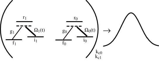
FIG. 1.: Schematic description of the cavity QED scheme proposed by Gheri et al. for the generation of polarization-entangled photon wave packets. The cavity and the relevant level structure of the atom trapped in it are shown.

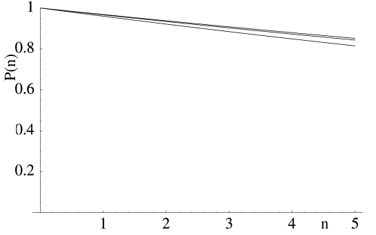
FIG. 2.: Fidelity of preparation $P(n)$ versus the number of entangled photons $n$ for different values of the relative fluctuations of the laser intensity $F_{r}$ (see Eq. (26)). The three curves refer, starting from the upper one, to $F_{r}=0,0.1,0.2$. Square laser pulses and identical parameters for the two polarizations have been considered. The other parameter values are: $g=\sqrt{I}=60$ MHz; $\delta=1500$ MHz; $k_{c}=25$ MHz; $T=30$ $\mu$sec.

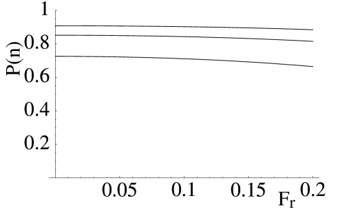
FIG. 3.: Fidelity of preparation $P(n)$ versus the the relative fluctuations of the laser intensity $F_{r}$ for different values of the number of generated entangled wavepackets $n$. The three curves refer, starting from the upper one, to $n=3,5,10$. Square laser pulses and identical parameters for the two polarizations have been considered. The other parameter values are the same as those of Fig. 2.

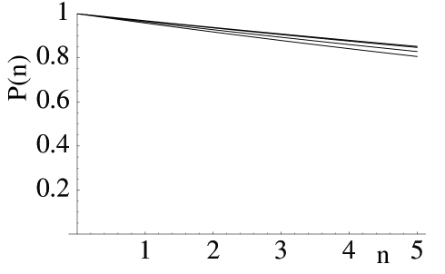
FIG. 4.: Fidelity of preparation $P(n)$ versus the number of photon wavepackets $n$ in the case of no laser intensity fluctuations but in the presence of photon losses with a rate $k_{a}$. The four curves refer to different values of the ratio of decay rates $k_{a}/k_{c}$: starting from the upper one, $k_{a}/k_{c}=0,0.001,0.005,0.01$. Square laser pulses and identical parameters for the two polarizations have been considered. The other parameter values are as in Fig. 2.

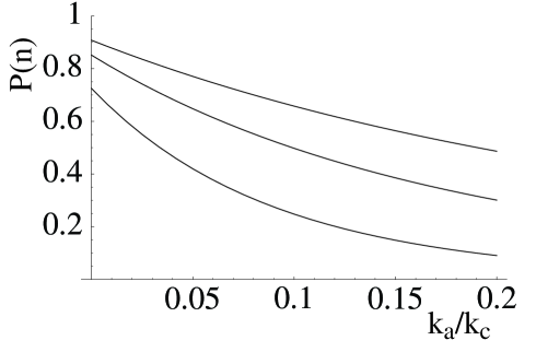
FIG. 5.: Fidelity of preparation $P(n)$ versus the ratio of decay rates $k_{a}/k_{c}$ for three different number of generated entangled wavepackets $n$. The three curves refer, starting from the upper one, to $n=3,5,10$. Square laser pulses and identical parameters for the two polarizations have been considered. The other parameter values are the same as those of Fig. 2.

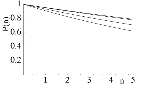
FIG. 6.: Fidelity of preparation $P(n)$ versus the number of photon wavepackets $n$ for different values of the effective initial mean vibrational thermal number $N$. The four curves refer, starting from the upper one, to $N=0.01,0.1,0.5,1$. The other parameters for the atomic motion are $\omega_{0}=1$ MHz and $\eta_{r}=\eta_{l}=0.07$, while the other parameter values are the same as those of Fig. 2. Square laser pulses and identical parameters for the two polarizations have been considered.

REFERENCES

- [1] A. Muller, H. Zbinden, and N. Gisin, Europhys. Lett. 33, 335 (1996); W.T. Buttler et al., Phys. Rev. Lett. 81, 3283 (1998).
- [2] D. Bouwmeester, J.-V. Pan, K. Mattle, M. Eibl, H. Weinfurter, and A. Zeilinger, Nature (London) 390, 575 (1997); D. Boschi, S. Branca, F. De Martini, L. Hardy, and S. Popescu, Phys. Rev. Lett. 80, 1121 (1998); A. Furusawa et al., Science 282, 706 (1998).
- [3] P. G. Kwiat, K. Mattle, H. Weinfurter, A. Zeilinger, A. V. Sergienko, Y. H. Shih, Phys. Rev. Lett. 75, 4337 (1995); P. G. Kwiat, E. Waks, A. G. White, I. Appelbaum, and P. H. Eberhard, Phys. Rev. A 60, R773 (1999).
- [4] D. M. Greenberger, M. A. Horne, and A. Zeilinger, Phys. Today 46, No. 8, 22 (1993).
- [5] D. Bouwmeester, J-W. Pan, M. Daniell, H. Weinfurter, and A. Zeilinger, Phys. Rev. Lett. 82, 1345 (1999).
- [6] C. K. Law and H. J. Kimble, J. Mod. Opt. 44, 2067 (1997).
- [7] A. Imamoğlu and Y. Yamamoto, Phys. Rev. Lett. 72, 210 (1994).
- [8] K. M. Gheri, C. Saavedra, P. Törma, J. I. Cirac, and P. Zoller, Phys. Rev. A 58, R2627 (1998).
- [9] C. W. Gardiner, Quantum Noise (Springer, Berlin, 1991).
- [10] F. Diedrich et al., Phys. Rev. Lett. 62, 403 (1989); C. Monroe et al., Phys. Rev. Lett. 75, 4011 (1995); E. Peik et al., Phys. Rev. A 60, 439 (1999); Ch. Roos et al., Phys. Rev. Lett. 83, 4713 (1999).
- [11] S.E. Hamann et al., Phys. Rev. Lett. 80, 4149 (1998); H. Perrin et al., Europhys. Lett. 42, 95 (1998).
- [12] D.J. Wineland, C. Monroe, W.M. Itano, D. Leibfried, B.E. King, D.M. Meekhof, J. Res. Natl. Inst. Stand. Technol. 103, 259 (1998).
- [13] T.A. Savard, K.M. O’Hara, and J.E. Thomas, Phys. Rev. A 56, R1095 (1997).
- [14] M. Hillery, V. Bužek, and A. Berthiaume, Phys. Rev. A 59,1829 (1999).
- [15] S. Bose, V. Vedral, and P. L. Knight, Phys. Rev. A 57, 822 (1998).