Quantum information processing in semiconductor nanostructures

Abstract

A major question for condensed matter physics is whether a solid-state quantum computer can ever be built. Here we discuss two different schemes for quantum information processing using semiconductor nanostructures. First, we show how optically driven coupled quantum dots can be used to prepare maximally entangled Bell and Greenberger-Horne-Zeilinger states by varying the strength and duration of selective light pulses. The setup allows us to perform an all-optical generation of the quantum teleportation of an excitonic state in an array of coupled quantum dots. Second, we give a proposal for reliable implementation of quantum logic gates and long decoherence times in a quantum dots system based on nuclear magnetic resonance (NMR), where the nuclear resonance is controlled by the ground state transitions of few-electron QDs in an external magnetic field. The dynamical evolution of these systems in the presence of environmentally-induced decoherence effects is also discussed.

	Phone	Fax
∗j.reina-estupinan@physics.ox.ac.uk	(44 1865) 272257	272400
†luis@anacaona.uniandes.edu.co	(57 1) 2839514	2839514
‡n.johnson@physics.ox.ac.uk	(44 1865) 272287	272400

1 Introduction

It has become increasingly clear that quantum mechanical principles are not just exotic theoretical statements but fundamental for a new technology of practical information processing [1]. Quantum computation, quantum cryptography and quantum teleportation represent exciting new arenas which exploit intrinsic quantum mechanical correlations.

The discovery of algorithms for which a computer based on the principles of quantum mechanics [2] should beat any traditional computer, has triggered intense research into realistic controllable quantum systems. Among the main areas involved in this active research field are ion traps [3], quantum electrodynamics cavities [4], nuclear magnetic resonance (NMR) [5], Josephson junctions [6] and semiconductor quantum dots (QDs) [7]. The main challenge now is to identify a physical system with an appropriate internal dynamics and corresponding external driving forces which enables one to selectively manipulate quantum superpositions and entanglements. A fundamental requirement for the experimental realization of such proposals is the successful generation of highly entangled quantum states. In particular, coherent evolution of two quantum bits (qubits) in an entangled state of the Bell type is fundamental to both quantum cryptography and quantum teleportation. Maximally entangled states of three qubits, such as the so-called Greenberger-Horne-Zeilinger (GHZ) states [8], are not only of intrinsic interest but are also of great practical importance in such proposals. Besides the capability to control and manipulate entanglement a great level of isolation from the environment is required to reach a full unitary evolution. Quantum information processing will be a reality when optimal control of quantum coherence in noisy environments can be achieved. The various communities typically rely on different hardware methodologies. Therefore, it is extremely important to clarify the underlying physics and limits for each type of physical realization of quantum information processing systems.

In this chapter we discuss two possible strategies using semiconductor QDs [9]. First, we review our main results on the optical generation and control of exciton entangled states in coupled QDs by using a state-of-the-art semiconductor setup that enables us to generate reliable maximally entangled states of $N$ qubits, starting from suitably initialized states. As an application of these exciton maximally entangled states, a true solid-state teleportation protocol is proposed. We show that the role of phonons, at low temperatures, in the driven QD system does not necessarily amount to the loss of control over the system due to destruction of coherence. Second, we address the implementation of a solid state NMR-based quantum switch. We discuss how the so-called “magic-number” transitions in few-electron QDs containing a nuclear spin impurity inside can be used to implement single qubit rotations and controlled$-$NOT (C$-$NOT) quantum gates. The basic setup consists of a nuclear spin-$\frac{1}{2}$ impurity placed at the center of a 2 electrons QD in the presence of an external perpendicular magnetic field $B$. In such a system, the nuclear magnetic resonance is controlled by the ground state transitions that arise as the $B$-field is changed: we show that the hyperfine coupling between the electrons and the nucleus can be changed and hence provide a mechanism for tuning the nuclear resonance frequency. Decoherence effects in systems of spin $\frac{1}{2}$ nuclei are expected to be minimal as nuclear spins are weakly coupled to their environment. Therefore, such spin systems are natural qubits for quantum information processing since they offer long decoherence times. Indeed they have been used in bulk liquid NMR experiments to perform some basic quantum algorithms like those of Deutsch [10] and Grover [11]. They have already been employed in some solid-state proposals, for example that of Ref. [12] where a set of donor atoms (like P) is embedded in pure silicon. Here, the qubit is represented by the nuclear spin of the donor atom and single qubit and C$-$NOT operations might then be achieved between neighbor nuclei by attaching electric gates on top and between the donor atoms [12]. Another proposal [13] suggests controlling the hyperfine electron-nuclear interaction via the excitation of the electron gas in quantum Hall systems. Both of these proposals, however, require the attachment of electrodes or gates to the sample in order to manipulate the nuclear spin qubit. Such electrodes are likely to have an invasive effect on the coherent evolution of the qubit, thereby destroying quantum information. In the second part of this chapter, we propose a NMR solid-state based mechanism for quantum computation free from these shortcomings. The outline of this chapter is as follows: In Section 2 we give a detailed prescription for producing maximally entangled exciton states of two and three semiconductor QDs. Section 3 considers the effects of decoherence on the optical generation of such entangled states. In Section 4, a protocol for teleporting the excitonic state of a quantum dot is proposed. In Section 5 we give a novel model for quantum logic with an NMR$-$based nanostructure switch. Concluding remarks are given in Section 6.

2 Generation of maximally entangled exciton states in optically driven quantum dots

When two quantum dots are sufficiently close, there is a resonant energy transfer process originating from the Coulomb interaction whereby an exciton can hop between dots [14]. Experimental evidence of such energy transfers between quantum dots was reported recently [15]; the resonant process also plays a fundamental role in biological and organic systems, and is commonly called the Förster process [16]. Unlike usual single-particle transport measurements, the Förster process does not require the physical transfer of the electron and the hole, just their energy. Hence it is relatively insensitive to the effects of impurities which lie between the dots.

Here we show how the resonant transfer (Förster) interaction between spatially separated excitons can be exploited to produce maximally entangled states of two (Bell) and three (GHZ) optically driven QDs, starting from suitably initialized states. Previous experiments have studied entangled states of trapped ions [3], photons [17], and particle spins in bulk liquid NMR [18], but to our knowledge, there is not such an scheme for producing deterministic entanglement in a semiconductor nanostructures setup. In the proposal given here we exploit recent experimental results involving coherent wavefunction control of excitons in semiconductor quantum dots on the nanometer and femtosecond scales [15, 19, 20, 21], i.e, the system requirements can be realized with current experiments employing both ultrafast and near-field optical spectroscopy of quantum dots.

We denote by 0 (1) a zero-exciton (single exciton) QD. We consider a system of $N$ identical and equispaced QDs, containing no net charge, which are radiated by long-wavelength classical light (see Figure 1) in order to produce reliable generation of the maximally entangled states $\left|\Psi_{Bell}(\varphi)\right\rangle={\textstyle{1\over\sqrt{2}}}(\left|00\right\rangle+e^{i\varphi}\left|11\right\rangle)\;$and $\left|\Psi_{GHZ}(\varphi)\right\rangle={\textstyle{1\over\sqrt{2}}}(\left|000\right\rangle+e^{i\varphi}\left|111\right\rangle)$, for several different values of the phase factor $\varphi$. The formation of single excitons within the individual QDs and their inter-dot hopping can be described in the frame of the rotating wave approximation (RWA) by the Hamiltonian ($\hbar=1$) [22]:

$$H_{{}_{\Lambda}}=\Delta_{\omega}J_{z}+A(J_{+}+J_{-})+W(J^{2}-J_{z}^{2})\ \ .$$ (1)

Here $\Delta_{\omega}\equiv\epsilon-\omega$ is the detuning parameter, $\epsilon$ is the QD band gap, $W$ represents the interdot Coulomb interaction (Förster process), the subscript $\Lambda$ refers to the rotating frame (see below), and the operators $J_{+}=\sum_{n=1}^{N}{e_{n}^{{\dagger}}h_{n}^{{\dagger}}}$, $J_{-}=\sum_{n=1}^{N}{h_{n}e_{n}}$, $J_{z}=\frac{1}{2}\sum_{n=1}^{N}{(e_{n}^{{\dagger}}e_{n}-h_{n}h_{n}^{{\dagger}})}$, with $e_{n}^{{\dagger}}$ ($h_{n}^{{\dagger}}$) describing the electron (hole) creation operator in the $n$’th QD. The  $J_{i}-$operators obey the usual angular momentum commutation relations $\left[J_{z},J_{\pm}\right]=\pm J_{\pm},\;\left[J_{+},J_{-}\right]=2J_{z},\;$and$\;[J^{2},J_{+}]=[J^{2},J_{-}]=[J^{2},J_{z}]=0,$ where $J^{2}\equiv{\textstyle{1\over 2}}[J_{+}J_{-}+J_{-}J_{+}]+J_{z}^{{}^{2}}$.  We consider the situation of a laser pulse with central frequency $\omega$ given by $\xi(t)=Ae^{-i\omega t}$, where $A$ gives the electron-photon coupling and the incident electric field strength. From a practical point of view, parameters $A\;$and $\Delta_{\omega}$ are adjustable in the experiment to give control over the system of QDs.

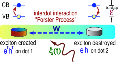
Figure 1: Schematic of the optical setup for the $N=2$ QDs system. The identical QDs, containing no net charge, are radiated with long-wavelength classical light of central frequency $\omega$, $\xi(t)=Ae^{-i\omega t}$. Formation of single excitons within the individual QDs and their inter-dot hopping in the presence of the Förster interaction are illustrated schematically. The bandgap $\epsilon$ as well as the conduction band (CB) and the valence band (VB) of the system are also shown.

Next, we discuss the main results obtained from the computation of both analytical and numerical solutions for the time evolution of $H_{{}_{\Lambda}}$ [22]. The solution to the quantum dynamical equation of motion of the system is equivalently given in terms of both the wave function and the density matrix formalisms, enabling us the strength and the length of the laser pulses required for reliably generation of maximally entangled exciton states of two and three QDs.

2.1 Unitary evolution and the wave function

The total wave function of the excitonic system considered here, starting with the initial condition $\left|\Psi(t=0)\right\rangle=\left|\Psi_{0}\right\rangle$ (for any $N$), can be expressed as $\left|\Psi(t)\right\rangle_{\Lambda}=\mathop{\textstyle\sum}_{k}C_{k}e^{-iE_{k}t}\left|\psi_{k}\right\rangle$, where $H\left|\psi_{k}\right\rangle=E_{k}\left|\psi_{k}\right\rangle$ ($H$ is the Hamiltonian in the laboratory frame), and $\left|\psi_{k}\right\rangle=\mathop{\textstyle\sum}_{j}A_{kj}\left|M_{j}\right\rangle.$ As mentioned before, the subscript $\Lambda$ refers to the unitary transformation which leads us from the laboratory frame to the rotating frame by using the rule $\left|\Psi(t)\right\rangle_{\Lambda}=\Lambda^{\dagger}(t)\left|\Psi(t)\right\rangle_{S}$, with $\Lambda=e^{-i\omega J_{Z}t}$ (subscript $S$ denotes Schrödinger picture). The normalization coefficients $C_{k}$ depend on the chosen initial condition $\left|\Psi_{0}\right\rangle$: by writing $\left|\Psi(0)\right\rangle=\mathop{\textstyle\sum}_{k}\beta_{k}\left|M_{k}\right\rangle$ $\left(\beta_{k}=\left\langle M_{k}\right.\left|\Psi(0)\right\rangle\right)$ we see, from the above expansion given for $\left|\Psi(t)\right\rangle_{\Lambda},$ that $\left|\Psi(0)\right\rangle=\mathop{\textstyle\sum}_{k}C_{k}\left|\psi_{k}\right\rangle.$ Hence, the general expression for the coefficients $C_{k}$ becomes $C_{k}=\left\langle\psi_{k}\right.\left|\Psi(0)\right\rangle=\mathop{\textstyle\sum}_{j}\beta_{j}\left\langle\psi_{k}\right.\left|M_{j}\right\rangle=\mathop{\textstyle\sum}_{j}\beta_{j}A_{kj}^{\ast}.$ The matrix elements $A_{kj}$ must be determined for each particular value of $N$, and $\left|M_{j}\right\rangle\equiv\left|J,M_{j};q\right\rangle$, where $J$ can take the values $\frac{N}{2},\frac{N}{2}-1,...,\frac{1}{2}\;$or$\;0$, and for each $J-$fixed value, we have the $2J+1$ different values $\;M=-\frac{N}{2},-\frac{N}{2}+1,...,\frac{N}{2}-1,\frac{N}{2}.$ The label $q\;$is introduced to further distinguish the states: $\ q=1,2,...,D_{J}$, where the multiplicity $D_{J}$, i.e. the number of states having angular momentum $J$ and $M=J$, is given by $D_{J}=\frac{2J+1}{J+\frac{N}{2}+1}{N\choose\frac{N}{2}+J}$. Hence, the total wave function in the rotating frame can be written as

$$\left|\Psi(t)\right\rangle_{\Lambda}=\sum_{k}{\sum_{j}C_{k}A_{kj}e^{-iE_{k}t}\left|M_{j}\right\rangle}\ \ .$$ (2)

The eigenfunction given in Eq. (2) describes any number of QDs. We only need to diagonalize a square matrix of side $2J+1$ for each $J$. Every eigenvalue so obtained occurs $D_{J}$ times in the entire spectrum. Next, we show how to generate highly excitonic entangled states by solving the quantum equation of motion associated with Eq. (2) for the cases $N=2$ and 3.

2.1.1 Two coupled QDs and Bell states

Here we give the light excitation procedure to obtain the maximally entangled Bell states $|\Psi_{Bell}(\varphi)\rangle=|00\rangle+e^{i\varphi}|11\rangle$. The phase $\varphi$ determines the type of entangled state generated in the optical process. We choose the basis of eigenstates of $J^{2}$ and $J_{z}$, $\{\left|M_{1}\right\rangle\equiv\left|J=1,M=-1\right\rangle\equiv\left|0\right\rangle$, $\left|M_{2}\right\rangle\equiv\left|J=1,M=0\right\rangle\equiv\left|1\right\rangle$, $\left|M_{3}\right\rangle\equiv\left|J=1,M=1\right\rangle\equiv\left|2\right\rangle\}$, as an appropriate representation for this problem. Here $|0\rangle$ represents the vacuum for excitons, $|1\rangle$ denotes the single-exciton state while $|2\rangle$ represents the biexciton state. In the absence of light, we have that $E(J,M)=\Delta_{\omega}M+W[J(J+1)-M^{2}]$, so the energy levels of the system are $E_{0}\equiv E(1,-1)=W-\Delta_{\omega}$, $E_{1}\equiv E(1,0)=2W$, and $E_{2}\equiv E(1,1)=W+\Delta_{\omega}$. Next, consider the action of the radiation pulse of light $\xi(t)$ over this pair of qubits at resonance, i.e. $\Delta_{\omega}=0$. In this case, the new eigen-energies of the coupled system are: $E_{0}=W,\;$and$\;E_{1,2}={\textstyle{1\over 2}}\Big{(}3W\pm\sqrt{16\left|A\right|^{2}+W^{2}}\Big{)}.$ Here we have assumed that the decoherence processes are negligibly small over the time scale of the evolution (see next section). It is a straightforward exercise to compute the explicit coefficients of Eq. (2) for both of the $J-$subspaces that span the Hilbert space $SU(2)\otimes SU(2)$ ($N=2$) [22]. Hence, the density of probability $\wp(Bell)\;$for finding the entangled Bell state between vacuum and biexciton states as a function of time for the initial condition $\left|\Psi_{0}\right\rangle=\left|0\right\rangle$ can be calculated as

$$\wp(Bell)={\textstyle{1\over 2}}\left|\mathop{\displaystyle\sum}_{k}C_{k}\left(A_{k1}+e^{i\varphi}A_{k3}\right)e^{-iE_{k}t}\right|^{2}.$$ (3)

Results of the computation of Eq. (3) are shown in Fig. 2. Here we show several different selective pulses of light $\tau_{{}_{B}}$ that produce the entangled state $|\Psi_{Bell}(\varphi=0)\rangle$. In these figures, energies are given in terms of the band gap $\epsilon$: $W=0.1$, and (a)$\;A={\textstyle{1\over 25}}$, (b)$\;A={\textstyle{1\over 50}}$, (c)$\;A=10^{-2}$, and (d)$\;A=10^{-3}$. Here the energy $W$ is kept fixed while the amplitude of the radiation pulse $A$ is varied.

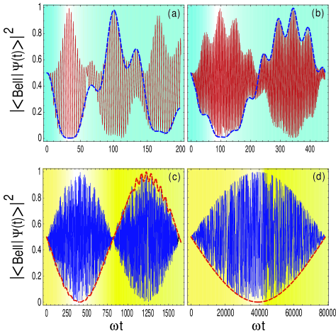
Figure 2: Generation of the Bell State ${\textstyle{1\over\sqrt{2}}}(\left|00\right\rangle+\left|11\right\rangle)$. These pulses correspond to the realization of the Hadamard gate followed by a quantum CNOT gate. $W=0.1$,$\;\varphi=0,\;$ and (a)$\;A={\textstyle{1\over 25}}$, (b)$\;A={\textstyle{1\over 50}}$, (c)$\;A=10^{-2}$, and (d)$\;A=10^{-3}$. $\left|\Psi(t)\right\rangle$ denotes the total wavefunction of the system at time $t$ in both laboratory (solid curves) and rotating frames (dashed curves). The energy is in units of the band gap $\epsilon$, and $\left|\Psi_{0}\right\rangle=\left|0\right\rangle$.

As a result of this, the time $\tau_{{}_{B}}$ increases with diminishing incident field strength $A$ [22]. We also consider another method for manipulating the length $\tau_{{}_{B}}$: keeping $A$ fixed while varying $W$. In this case, the analysis shows that for a fixed value of $A$ the length $\tau_{{}_{B}}$ decreases with decreasing interaction strength $W$ [22]. The latter procedure could be experimentally more expensive than the former since the variation of $W$ has to be tailored by changing the interdot distance and/or the radius of the dots. However, this method offers an interesting experimental possibility for studying the Förster mechanism.

Regarding the experimental generation of these Bell states, we suggest a consideration of wide-gap semiconductor QDs, like ZnSe based QDs, for instance. For these materials, the band gap $\epsilon=2.8\;$ eV, which implies a resonant optical frequency $\omega=4.3\times 10^{15}$ s^-1. Femtosecond spectroscopy is currently available for these systems[20]. For a $\varphi=0$ or $2\pi$ pulse, $W=0.1$ $\epsilon\;$and$\;A=0.04$ $\epsilon$, it can be seen from Fig. 2(a) that the generation of the state ${\textstyle{1\over\sqrt{2}}}\left(\left|00\right\rangle+\left|11\right\rangle\right)$ requires a pulse of length $\tau_{{}_{B}}=7.7\times 10^{-15}$ s. By changing the value of the amplitude $A$, we can modify the length $\tau_{{}_{B}}$ of this Bell pulse, i.e. a new $A$ implies a new value for $\tau_{{}_{B}}$: from Fig. 2 we can see that $\tau_{{}_{B}}$ can be tailored in such a way that reliable entangled state preparation can be done in the interval $10^{-11}$ s $<\tau_{{}_{B}}<10^{-15}$ s [22], which is in agreement with currently available excitonic dephasing times [19].

2.1.2 Three coupled QDs and GHZ states

We give the procedure for generating the entangled GHZ states $\left|\Psi_{GHZ}(\varphi)\right\rangle={\textstyle{1\over\sqrt{2}}}(\left|000\right\rangle+e^{i\varphi}\left|111\right\rangle),$ for arbitrary values of $\varphi,$ in the proposed system of $3$ coupled QDs. Without loss of generality, we consider the $J=\frac{3}{2}-$subspace as the only one optically active (the other two $J=1/2$ subspaces remain optically dark). We work in the basis set $|J=3/2,M\rangle$, $\{|0\rangle=|3/2,-3/2\rangle$, $|1\rangle=|3/2,-1/2\rangle$, $|2\rangle=|3/2,1/2\rangle$, $|3\rangle=|3/2,3/2\rangle\}$, where $|0\rangle$ is the vacuum state, $|1\rangle$ is the single-exciton state, $|2\rangle$ is the biexciton state and $|3\rangle$ is the triexciton state. In the absence of light, the energy levels of the system are given by $E_{0}\equiv E(3/2,-3/2)={\textstyle{3\over 2}}(W-\Delta_{\omega})$, $E_{1}\equiv E(3/2,-1/2)={\textstyle{1\over 2}}(7W-\Delta_{\omega})$, $E_{2}\equiv E(3/2,1/2)={\textstyle{1\over 2}}(7W+\Delta_{\omega})$, and $E_{3}\equiv E(3/2,3/2)={\textstyle{3\over 2}}(W+\Delta_{\omega})$. Next we consider, at resonance, the effect of the pulse of light $\xi(t)$ over this system of 3 QDs: we get the new eigenenergies $E_{0,1}={\textstyle{5\over 2}}W+\left|A\right|\pm\sqrt{\left(W+\left|A\right|\right)^{2}+3\left|A\right|^{2}},$ and $E_{2,3}={\textstyle{5\over 2}}W-\left|A\right|\pm\sqrt{\left(W-\left|A\right|\right)^{2}+3\left|A\right|^{2}}.$

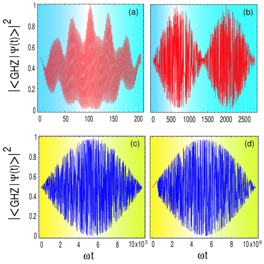
Figure 3: Generation of the GHZ state ${\textstyle{1\over\sqrt{2}}}(\left|000\right\rangle+\left|111\right\rangle)$. These pulses correspond to the realization of the Hadamard gate followed by two quantum CNOT gates. $W=0.1$,$\;\varphi=0,\;$ and (a)$\;A={\textstyle{1\over 25}}$, (b)$\;A={\textstyle{1\over 50}}$, (c)$\;A=10^{-2}$, and (d)$\;A=10^{-3}$.

Starting with a zero-exciton state as the initial state, i.e. $\left|\Psi_{0}\right\rangle=\left|0\right\rangle$, we calculate the probability density $\wp(GHZ)\;$of finding the entangled $\left|\Psi_{GHZ}(\varphi)\right\rangle$ state between vacuum and triexciton states as

$$\wp(GHZ)={\textstyle{1\over 2}}\left|\mathop{\displaystyle\sum}_{k}C_{k}\left(A_{k1}+e^{i\varphi}A_{k4}\right)e^{-iE_{k}t}\right|^{2}.$$ (4)

In Figure 3 the selective pulses used to generate the GHZ state ${\textstyle{1\over\sqrt{2}}}\left(\left|000\right\rangle+\left|111\right\rangle\right)$ ($\varphi=0,2\pi$) are shown: it can be seen from Fig. 3(a) that for a band gap $\epsilon=2.8\;$eV (resonant optical frequency $\omega=4.3\times 10^{15}$ s^-1), $W=0.1$ $\epsilon\;$and$\;A={\textstyle{\epsilon\over 25}}$, a pulse of length $\tau_{{}_{GHZ}}=1.3\times 10^{-14}$ s is required. We explore several different ranges for the $\tau_{{}_{GHZ}}-$pulses required in the generation of these GHZ states. For fixed $W,$ the time $\tau_{{}_{GHZ}}$ increases with decreasing incident field strength $A.$ In contrast, for fixed $A,$ the length $\tau_{{}_{GHZ}}$ decreases with decreasing interdot interaction strength [22]. It is worth noting that after the preparation step, which is determined by the length of the pulses $\tau_{{}_{Bell}}$ and $\tau_{{}_{GHZ}}$, the Förster interaction parameter $W$, and the field strength $A$, the system will evolve under the action of the Hamiltonian (1) with $\Delta_{\omega}=A=0$: each one of the maximally entangled states discussed here are eigenstates of this remaining Hamiltonian.

The above results are not restricted to ZnSe-based QDs: by employing semiconductors of different bandgap $\epsilon$ (e.g., GaAs, organic-inorganic systems), other regions of parameter space can be explored. We have studied the time evolution of the system of QDs for several different values of the phase $\varphi$. These give similar qualitative results to the ones discussed previously. Next, we show how the density matrix formalism can be used in an equivalent manner in order to produce the excitonic entangled states described before.

2.2 Pseudo-spin operators and the density matrix

In this section we consider a rectangular radiation pulse, starting at time $t=0$ with central frequency $\omega$, given by $\xi(t)={\it A}{\rm cos}(\omega t)$. The time evolution of any initial state under the action of the Hamiltonian (1) is easily performed by means of the pseudo $\frac{1}{2}-$spin operator formalism[23, 24]. Single transition operators are defined by

$$\langle i|J_{x}^{r-s}|j\rangle=\frac{1}{2}(\delta_{ir}\delta_{js}+\delta_{is}\delta_{jr}),\ \ \langle i|J_{y}^{r-s}|j\rangle=\frac{i}{2}(-\delta_{ir}\delta_{js}+\delta_{is}\delta_{jr}),\ \ \langle i|J_{z}^{r-s}|j\rangle=\frac{1}{2}(\delta_{ir}\delta_{jr}-\delta_{is}\delta_{js})$$ (5)

where $r$-$s$ denotes the transition between states $|r\rangle$ and $|s\rangle$ within a given $J$ subspace. The three operators belonging to one particular transition $r$-$s$ obey standard angular momentum commutation relationships $\left[J_{\alpha}^{r-s},J_{\beta}^{r-s}\right]=iJ_{\gamma}^{r-s}$, where $(\alpha,\beta,\gamma)$ represents a cyclic permutation of $(x,y,z)$ (operators belonging to non-connected transitions commute: $\left[J_{\alpha}^{r-s},J_{\beta}^{t-u}\right]=0$ with $\alpha,\beta=x,y$ or $z$). In this case, the Hamiltonian in the rotating frame ($\epsilon\gg W$) becomes

$$H_{{}_{\Lambda}}=\Delta_{\omega}J_{z}-{\textstyle{1\over 2}}A(J_{+}+J_{-})-W(J^{2}-J_{z}^{2}).$$ (6)

We now give the expressions for the density matrix associated with the $N=2,3$ QD systems and show that the Hamiltonian (6) leads to the generation of the entangled states $\left|\Psi_{Bell}(\varphi)\right\rangle,$ and $\left|\Psi_{GHZ}(\varphi)\right\rangle.$

2.2.1 Bell states

Here we describe the light excitation procedure to obtain the Bell-type states $|\Psi_{Bell}(\varphi)\rangle$. To find the analytical solution of the dynamical equation governing the system’s matrix density, we start with the initial condition representing the vacuum of excitons: only the $J=1$ subspace is optically active (the $J=0$ subspace remains dark). Choosing the basis of eigenstates of $J^{2}$ and $J_{z}$ as in Section 2.1.1, the rotating frame Hamiltonian and initial density matrix can be expressed in terms of pseudo-spin operators as follows

$$H_{{}_{\Lambda}}=-2\Delta_{\omega}J_{z}^{0-2}+{\textstyle{2W\over 3}}(J_{z}^{0-1}-J_{z}^{1-2})-\sqrt{2}A(J_{x}^{0-1}+J_{x}^{1-2})\ \ ,$$

$$\rho(0)={\textstyle{1\over 3}}I+{\textstyle{2\over 3}}(J_{z}^{0-1}+J_{z}^{0-2})\ \ .$$ (7)

Here $I$ denotes the identity matrix in the subspace $J=1$. In the absence of light, the energy levels of the system are given as in Section 2.1.1 (with accuracy of a sign). Consider the action of a pulse of light at resonance and amplitude $A\ll W$. Assuming that the decoherence processes are negligibly small over the time scale of the evolution (see later), the density matrix at time $t$ becomes

$$\rho(t)={\textstyle{1\over 3}}I+\left[{\rm cos}(\omega_{2}t)+{\textstyle{1\over 3}}\right]J_{z}^{0-1}+\left[{\rm cos}(\omega_{2}t)-{\textstyle{1\over 3}}\right]J_{z}^{1-2}-{\rm sin}(\omega_{2}t)J_{y}^{0-2}\ \ ,$$ (8)

which exhibits the generation of coherence between vacuum and biexciton states through the operator $J_{y}^{0-2}$, which oscillates at frequency $\omega_{2}=A^{2}/W$.

The state $|\Psi_{Bell}(\varphi)\rangle$ has a corresponding density matrix $\rho_{Bell}=I/3+J_{z}^{0-1}/3-J_{z}^{1-2}/3+{\rm cos}(\varphi)J_{x}^{0-2}-{\rm sin}(\varphi)J_{y}^{0-2}$. Comparing this last equation with Eq. (8), we see that the system’s quantum state at time $\tau_{B}=\pi W/2A^{2}$ corresponds to the maximally entangled Bell state $|\Psi_{Bell}(\pi/2)\rangle$. The time evolutions of populations and coherences for an initial vacuum state are plotted in Fig. 4. The evolution of populations of the vacuum $\rho_{00}$ and the biexciton $\rho_{22}$ states are shown in Fig. 4(a). Clearly the approximate analytic calculation given here describes the system’s evolution very well when compared with the exact numerical solution (Fig. 4(a)). Figure 4(b) shows the overlap, $O(t)=Tr\left[\rho_{Bell}\rho(t)\right]$, between the maximally entangled Bell state and the one obtained by applying a rectangular pulse of light at resonance. The thick solid line (Fig. 4(b)) describes $O(t)$ with a maximally entangled Bell state in the rotating frame, while the thin solid line (Fig. 4(b)) represents the overlap with a Bell state transformed to the laboratory frame: obviously the rotating frame case corresponds to the amplitude evolution of the laboratory frame signal. The dashed line illustrates the approximate solution overlap in the rotating frame. The approximate solution works very well, supporting the idea that a selective Bell pulse of length $\tau_{B}=\pi W/2A^{2}$ can be used to create the Bell state $|\Psi_{Bell}(\pi/2)\rangle$ in the system of two coupled QDs. The same conclusion can also be drawn from the time evolution of the overlap between the exact Bell-state density matrix and the one obtained directly from the numerical calculation [22](b). Therefore, the existence of a selective Bell pulse is numerically confirmed.

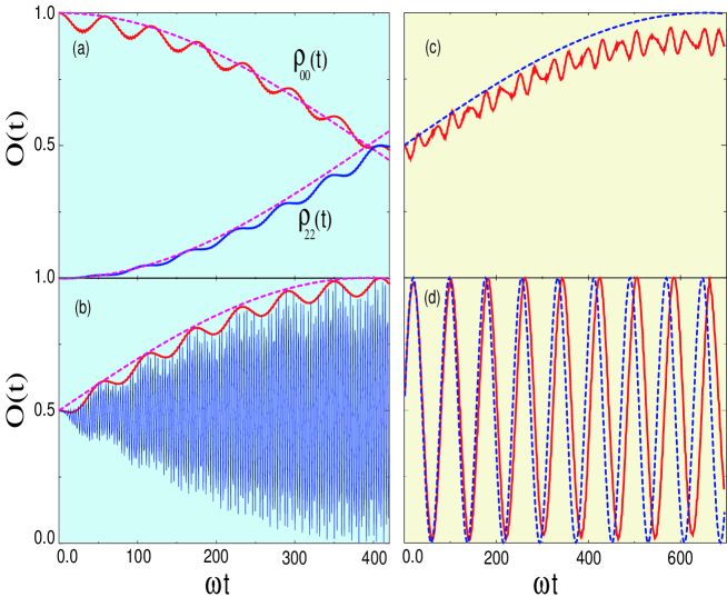
Figure 4: (a) Population of the vacuum state $\rho_{00}$ and biexciton state $\rho_{22}$ in two coupled QDs, as a function of time. (b) Time-evolution of overlap with maximally entangled Bell state. $\epsilon=1$, $W=\epsilon/10$ and $A=W/5$. Blue (thin solid) line shows exact numerical result in the laboratory frame. Red (thick solid) line in (b) represents the exact numerical solution in the rotating frame. Pink (dashed) line shows approximate analytical result. (c) Time-evolution of overlap with maximally entangled $GHZ$ states $\left|\Psi_{GHZ}(\varphi)\right\rangle$, and (d) $\left|\Psi_{GHZ}(\varphi)\right\rangle_{2}$, under the action of a rectangular pulse of light at resonance. $\epsilon=1$, $W=\epsilon/10$ and $A=2W/5$. Red (solid) line represents exact numerical solution. Blue (dashed) line shows approximate analytical result.

2.2.2 GHZ states

Next, consider three quantum dots of equal size placed at the corners of an equilateral triangle, as in Section 2.1.2, with the $J=\frac{3}{2}$ subspace being the only one optically active subspace, and with the same basis set of Section 2.1.2. In terms of pseudo-spin operators, the rotating frame Hamiltonian, including the radiation term, is now given by

$$H_{{}_{\Lambda}}=-\Delta_{\omega}(3J_{z}^{0-3}+J_{z}^{1-2})+2W(J_{z}^{0-1}-2J_{z}^{2-3})-A\left[\sqrt{3}(J_{x}^{0-1}+J_{x}^{2-3})+2J_{x}^{1-2}\right]\ \ .$$ (9)

In terms of its associated density matrix, the entangled state $\left|\Psi_{GHZ}(\varphi)\right\rangle$ between vacuum and triexciton states is given by $\rho_{GHZ}=I/4+J_{z}^{0-1}/2-J_{z}^{2-3}/2+{\rm cos}(\varphi)J_{x}^{0-3}+{\rm sin}(\varphi)J_{y}^{0-3}$, where $I$ denotes the identity matrix in the $J=\frac{3}{2}$ subspace. This state can be generated after an appropriate $\frac{\pi}{2}-$pulse: starting with a zero-exciton state $|0\rangle$, at resonance, and using the properties of pseudo-spin operators, the evolved state under the action of Hamiltonian Eq. (9) can be obtained in a straighforward way in the limit $A/W\ll 1$ [22](b):

$$\rho(t)={\textstyle{1\over 4}}I+\left[{\rm cos}(\omega_{3}t)+{\textstyle{1\over 2}}\right]J_{z}^{0-1}+{\rm cos}(\omega_{3}t)J_{z}^{1-2}+\left[{\rm cos}(\omega_{3}t)-{\textstyle{1\over 2}}\right]J_{z}^{2-3}+{\rm sin}(\omega_{3}t)J_{y}^{0-3}\ \ ,$$ (10)

with $\omega_{3}=d_{-}-d_{+}+A$ and $d_{\pm}=W\left[1\pm\frac{A}{W}+(\frac{A}{W})^{2}\right]^{1/2}$. Clearly $|\Psi_{GHZ}(\pi/2)\rangle$ can be generated with a $\frac{\pi}{2}-$pulse of length $\tau_{GHZ}=4\pi W^{2}/3A^{3}$. In Fig. 4(c) we show the overlap between the exact density matrix and that corresponding to state $\left|\Psi_{GHZ}(\varphi)\right\rangle$. The dashed line shows the overlap using our approximate density matrix, Eq. (10).

We also give the scheme for generating the entangled state between a single exciton $|1\rangle$ and the biexciton $|2\rangle$, $\left|\Psi_{GHZ}(\varphi)\right\rangle_{2}=\frac{1}{\sqrt{2}}(|1\rangle+e^{i\varphi}|2\rangle)$. In order to generate $\left|\Psi_{GHZ}(\varphi)\right\rangle_{2}$, we take the single exciton state $|1\rangle$ as the initial condition. Evolution of this new initial state under $H_{{}_{\Lambda}}$ (Eq. (9)) with $\Delta_{\omega}=0$ generates a new density matrix $\rho(t)$ which can be used to show that a pulse of duration $\tau_{GHZ}^{\prime}=\pi/4A$, generates the state $\left|\Psi_{GHZ}(\pi/2)\right\rangle_{2}$. Figure 4(d) shows the overlap between $\rho(t)$ and $\rho_{GHZ_{2}}$ [22](b). We emphasize that the two maximally entangled GHZ states considered above have very different frequencies. This feature should enable each of these maximally entangled $GHZ$ states to be manipulated separately in actual experiments, even if the initial state is mixed.

From the results above, it follows that in order to generate maximally entangled exciton states, $\frac{\pi}{2}-$pulses with sub-picosecond duration should be used. A surprising conclusion of our results is that entangled-state preparation is facilitated by weak light fields (i.e. $A\ll W$): strong fields cause excessive oscillatory behavior in the density matrix. The relevant experimental conditions as well as the required coherent control to realize the above combinations of parameters, are compatible with those demonstrated in Refs. [15, 19, 20]: we expect that the experimental generation of the Bell and GHZ states discussed here should be possible with these ultrafast semiconductor optical techniques. Here it is important to highlight that the corresponding increase in the effective gap will yield a larger exciton binding energy: typical decoherence mechanisms (e.g., acoustic phonon scattering) will hence become less effective. The generation of maximally entangled states in this proposal has considered the experimental situation of global excitation pulses, i.e. pulses acting simultaneously on the entire QD system. However, by using near-field optical spectroscopy [21], individual QDs from an ensemble can be addressed by using local pulses, a feature that can be exploited to generate entangled states with different symmetries, such as the antisymmetric state ${\textstyle{1\over\sqrt{2}}}(\left|01\right\rangle-\left|10\right\rangle).\;$ Hence, we should be able to generate the so-called Bell basis of four mutually orthogonal states for the 2 qubits, all of which are maximally entangled, i.e. the set of states ${\textstyle{1\over\sqrt{2}}}\{(\left|00\right\rangle+\left|11\right\rangle),\;(\left|00\right\rangle-\left|11\right\rangle),\;(\left|01\right\rangle+\left|10\right\rangle),\;(\left|01\right\rangle-\left|10\right\rangle)\}$.  From a general point of view, this basis is of fundamental relevance for quantum information processing.

In summary, we have shown how maximally entangled Bell and GHZ states can be generated using the optically driven resonant transfer of excitons between quantum dots. Selective Bell and GHZ pulses have been identified by an approximate, yet accurate, analytical approach which should prove a useful tool when designing experiments. Exact numerical calculations confirm the existence of such $\varphi-$pulses for the generation of maximally entangled states in coupled dot systems.

3 Decoherence mechanisms

Here we analize the reliability of the preparation of entangled states when decoherence mechanisms are taken into account during the generation step. Exciton decoherence in semiconductor QDs is dominated by acoustic phonon scattering at low temperatures [26]. Hence, we consider the acoustic phonon dephasing mechanism

$$H_{env}=\sum_{\vec{k}}{\omega_{\vec{k}}a_{\vec{k}}^{{\dagger}}a_{\vec{k}}}+\sum_{\vec{k}}{g_{\vec{k}}J_{z}(a_{\vec{k}}^{{\dagger}}+a_{\vec{k}})},$$ (11)

where $a_{\vec{k}}^{{\dagger}}$ ($a_{\vec{k}}$) is the creation (annihilation) operator of the acoustic phonon with wavevector ${\vec{k}}$, as the main factor responsible for decoherence effects in the generation of the maximally entangled exciton states analized before [27]. The new time evolution to be analyzed is modelled by the Hamiltonian $H^{\prime}=H_{{}_{\Lambda}}+H_{env}$.

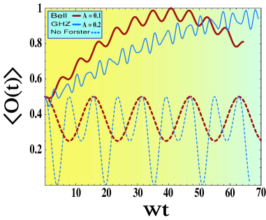
Figure 5: Maximally entangled exciton states generation in the zero decoherence limit. Thick (red) lines represent the Bell-state overlap with $A=0.1$: solid, Forster term included; dotted, Forster term not included. Thin (blue) lines represent the GHZ-state overlap with $A=0.2$ and same meaning for solid and dotted lines.

Here we consider pure decoherence effects that do not involve energy relaxation of excitons (these effects will be addressed elsewhere [29]). The exact kinetic equations for the system of QDs can be obtained by applying the method of operator-equation hierarchy developed for Dicke systems in [28]. Following the standard procedure, by assuming a very short correlation time for exciton operators, the exact hierarchy of equations transforms into a Markovian master equation. The initial condition is represented by the density matrix $\rho(0)=|0\rangle\langle 0|\rho_{Ph}(T)$, exciton vacuum and the equilibrium phonon reservoir at temperature $T$. At resonance ($\Delta_{\omega}=0$) the dynamical equation for the expectation value of exciton operators is given by

$$\frac{\partial\langle J_{\alpha}^{r-s}\rangle}{\partial t}=-iW\langle[J_{\alpha}^{r-s},J_{z}^{2}]\rangle-iA\langle[J_{\alpha}^{r-s},J^{+}+J^{-}]\rangle-\Gamma(2\langle[J_{\alpha}^{r-s},J_{z}]J_{z}\rangle-\langle[J_{\alpha}^{r-s},J_{z}^{2}]\rangle),$$ (12)

where $\Gamma=\int{d\omega^{\prime}\omega^{\prime n}e^{-\omega^{\prime}/\omega_{c}}(1+2N(\omega^{\prime},T))}$ is the decoherence rate with $n$ depending on the dimensionality of the phonon field, $\omega_{c}$ is a cut-off frequency (typically the Debye frequency) and $N(\omega^{\prime},T)$ is the phonon Bose-Einstein occupation factor. It is a well known fact that very narrow linewidth of the photoluminescence signal of a single QD does exist due to the elimination of inhomogeneous broadening effects. Consequently, the decoherence rate $\Gamma$ in this analysis should be associated with just homogeneous broadening effects. At low temperature the main decoherence mechanism is indeed acoustic phonon scattering processes. The decoherence parameter $\Gamma$ is temperature dependent and it amounts to 20-50 $\mu$eV for typical III-V semiconductor QDs in a temperature range from 10 K to 30 K [26]. We consider typical values for $\Gamma$ which can represent real situations for QDs at low temperatures together with the experimental conditions $\epsilon=\omega=1$ and the Förster term $W=0.1$ $\epsilon$. Laser strengths and decoherence rates are expressed in units of $W$. The coupled differential linear equations for the time dependent pseudo-spin expectation values are solved and the results are given in terms of the time dependent overlaps $O_{B}(t)=Tr\{\rho_{Bell}\rho(t)\}$ and $O_{GHZ}(t)=Tr\{\rho_{GHZ}\rho(t)\}$ [27].

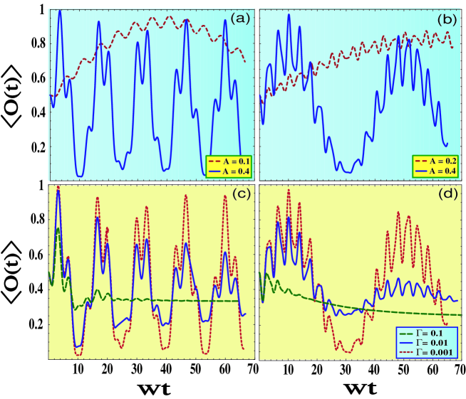
Figure 6: Maximally entangled exciton states generation in the presence of decoherence: (a) $\langle O_{B}(t)\rangle$ for $A=0.1$, red (dotted) line and $A=0.4$, blue (solid) line. (b) $\langle O_{G}(t)\rangle$ for $A=0.2$, red (dotted) line and $A=0.4$, blue (solid) line. In plots (a) and (b) $\Gamma$ is kept fixed: $\Gamma=0.001$. In figures (c) and (d) $A=0.4$ is kept fixed whereas $\Gamma$ is varied: $\Gamma=0.001$, red (dotted) line, $\Gamma=0.01$, blue (solid) line and $\Gamma=0.1$, green (dashed) line. These curves correspond to (c) $\langle O_{B}(t)\rangle$ and (d) $\langle O_{G}(t)\rangle$.

Figure 5 shows the evolution of the overlaps $O_{B}(t)$ and $O_{GHZ}(t)$ in the limit of very weak light excitation and zero decoherence. It can be seen that no maximally entangled exciton states generation is possible if the Förster interaction is turned off. This implies that efficient exciton entangled states generation should be helped by compact QD systems where the Förster term can take a significant value, as we discussed in the above section. Figures 6(a) and 6(c) show the case of Bell-state generation ($N=2$ QDs) in the presence of noise. In Fig. 6(a) the decoherence rate $\Gamma=0.001$, and the laser intensities are $A=0.1$, and $A=0.4$. It is shown that $\tau_{B}$ is significantly shortened by applying stronger laser pulses. Therefore, decoherence effects can be minimized by using higher excitation levels. However, a higher laser intensity also implies a sharper evolution which therefore requires a very precise pulse length. Figure 6(c) shows temperature-dependent results for $\Gamma=0.001$, 0.01 and 0.1, when $A=0.4$ is kept fixed. We can see that at high temperatures ($\Gamma=0.1$) no maximally entangled states generation is possible. However, it can be estimated that $\Gamma$ values between $0.001-0.01$ are typical in the temperature range from $10$ K to $50$ K: in this parameter window successful generation of Bell states can be produced [27], as shown in Fig. 6(c). Figures 6(b) and 6(d) show the case of GHZ states generation ($N=3$ QDs). As above, $\tau_{GHZ}$ is shortened by using higher laser excitation levels, as can be seen from Fig. 6(b) for $\Gamma=0.001$. Figure 6(d) shows the temperature effects through the variation of $\Gamma$ for $A=0.4$. We see that similar decoherence rates yield a more dramatic reduction of the coherence in the GHZ case than in the Bell case. However, as for Bell generation, a parameter window does exist where the generation of such entangled states are feasible [27]. It is worth noting the different scaling behaviour of the generation frequency of these entangled states at very low temperature, i.e. vanishing $\Gamma$ and very low laser excitation. While selective $\frac{\pi}{2}$ laser pulse length for the Bell case scales like $W/A^{2}$, selective $\frac{\pi}{2}$ pulse length for the GHZ case scales like $W^{2}/A^{3}$. This property of $\frac{\pi}{2}$ pulses to generate maximally entangled exciton states was demonstrated analytically in the above section and is verified in the present section by looking at the numerical results presented in Figure 6.

In summary, decoherence effects can be minimized in the generation of maximally entangled states by applying stronger laser pulses and working at low temperatures where acoustic phonon scattering is the main decoherence mechanism. Since we have shown that the generation of maximally entangled exciton states is preserved over a reasonable parameter window even in the presence of decoherence mechanisms, we stress that this optical generation could be exploited in solid state devices to perform quantum protocols, such as the teleportation of an excitonic state in a coupled QD system [30], as we show next.

4 Quantum teleportation of excitonic states

Here we propose a practical scheme capable of demonstrating quantum teleportation which exploits currently available ultrafast spectroscopy techniques in order to prepare and manipulate entangled states of excitons in coupled QDs [30]. Since the original idea of quantum teleportation considered in 1993 by Bennett et al. [31], great efforts have been made to realize the physical implementation of teleportation devices [32]. The general scheme of teleportation [31], which is based on Einstein-Podolsky-Rosen (EPR) pairs [33] and Bell measurements [34] using classical and purely nonclassical correlations, enables the transportation of an arbitrary quantum state from one location to another without knowledge or movement of the state itself through space. This process has been explored from various points of view [32]; however none of the experimental set-ups to date have considered a solid-state approach, despite the recent advances in semiconductor nanostructure fabrication and measurement [9, 15, 19, 21]. Reference [19], for example, demonstrates the remarkable degree of control which is now possible over quantum states of individual quantum dots (QDs) using ultra-fast spectroscopy. The possibility therefore exists to use optically-driven QDs as “quantum memory” elements in quantum computation operations, via a precise and controlled excitation of the system.

In order to implement the quantum operations for the description of the teleportation scheme proposed here, we employ two elements: the Hadamard transformation and the quantum controlled-NOT gate (C-NOT gate). In the orthonormal computation basis of single qubits $\left\{\left|0\right\rangle,\left|1\right\rangle\right\}$, the C-NOT gate acts on two qubits $\left|\varphi_{i}\right\rangle$ and $\left|\varphi_{j}\right\rangle$ simultaneously as follows: C-NOT${}_{ij}(\left|\varphi_{i}\right\rangle\left|\varphi_{j}\right\rangle)\mapsto\left|\varphi_{i}\right\rangle\left|\varphi_{i}\oplus\varphi_{j}\right\rangle$. Here $\oplus$ denotes addition modulo 2. The indices $i$ and $j$ refer to the control bit and the target bit respectively (see Fig. 7). The Hadamard gate $U_{H}$ acts only on single qubits by performing the rotations $U_{H}(\left|0\right\rangle)\mapsto\frac{1}{\sqrt{2}}\left(\left|0\right\rangle+\left|1\right\rangle\right)$ and $U_{H}(\left|1\right\rangle)\mapsto\frac{1}{\sqrt{2}}\left(\left|0\right\rangle-\left|1\right\rangle\right)$. The above unitary transformations can be written as

$$U_{H}={\textstyle{1\over\sqrt{2}}}\left(\matrix{1&~{}~{}1\cr 1&-1\cr}\right),\ \ C-NOT=\left(\matrix{1&0&0&0\cr 0&1&0&0\cr 0&0&0&1\cr 0&0&1&0\cr}\right)\ \ ,$$ (13)

and represented in the language of quantum circuits as in Figure 7.

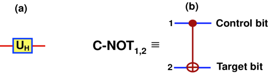
Figure 7: Schematic representation of (a) The Hadamard gate, and (b) The controlled-NOT gate.

We also introduce a pure state $\left|\Psi\right\rangle$ in this Hilbert space given by $\left|\Psi\right\rangle=\alpha\left|0\right\rangle+\beta\left|1\right\rangle$ with $\left|\alpha\right|^{2}+\left|\beta\right|^{2}=1$, where $\alpha\;$and $\beta\;$are $\mathop{\rm complex}$ numbers. As discussed in the above section, $\left|0\right\rangle$ represents the vacuum state for excitons while $\left|1\right\rangle$ represents a single exciton. Following Ref. [35], in Figure 8 we show the general computational approach discussed in this section. As usual, we refer to two parties, Alice and Bob. Alice wants to teleport an arbitrary, unknown qubit state $\left|\Psi\right\rangle$ to Bob. Figure 9 shows the specific realization we are proposing using optically controlled quantum dots with QD $a$ initially containing $\left|\Psi\right\rangle$. Alice prepares two qubits (QDs $b$ and $c$) in the state $\left|0\right\rangle$ and then gives the state $\left|\Psi 00\right\rangle$ as the input to the system. By performing the series of transformations shown in Fig. 8, Bob receives as the output of the circuit the state ${\textstyle{1\over\sqrt{2}}}(\left|0\right\rangle+\left|1\right\rangle)_{a}{\textstyle{1\over\sqrt{2}}}(\left|0\right\rangle+\left|1\right\rangle)_{b}\left|\Psi\right\rangle_{c}$ (Fig. 9(d)). In Ref. [30] we generalize the teleportation scheme given in Ref. [35] to the case of an $N$ qubit quantum circuit. In order to describe the physical implementation of the quantum circuit given in Fig. 8 using coupled quantum dots, we exploit the recent experimental results involving coherent control of excitons in single quantum dots on the nanometer and femtosecond scales [19, 15]. Consider a system of three identical and equispaced QDs containing no net charge (Fig. 9(a)), which are initially prepared in the state $\left|\Psi\right\rangle_{a}\left|0\right\rangle_{b}\left|0\right\rangle_{c}$. As shown in Fig. 9(a), one of these (QD $a$) contains the quantum state $\left|\Psi\right\rangle_{a}$ that we wish to teleport, while the other two (QDs $b$ and $c$) are initialized in the state $\left|00\right\rangle_{bc}-$ this latter state is easy to achieve since it is the ground state. Following this initialization, we illuminate QDs $b$ and $c$ with the radiation pulse $\xi(t)=A\exp(-i\omega t)$ (see Fig. 9(b)). For the case of ZnSe-based QDs, the band gap $\epsilon=2.8$ eV, hence the resonance optical frequency $\omega=4.3\times 10^{15}$ s^-1. For a $0$ or $2\pi-$pulse, the density of probability for finding the QDs $b$ and $c$ in the Bell state ${\textstyle{1\over\sqrt{2}}}\left(\left|00\right\rangle+\left|11\right\rangle\right)$ requires the length $\tau_{{}_{Bell}}=7.7\times 10^{-15}$ s (see Fig. 2(a)). Hence, this time $\tau_{{}_{Bell}}$ corresponds to the realization of the first two gates of the circuit in Fig. 8, i.e. the Hadamard transformation over QD $b$ followed by the C-NOT gate between QDs $b$ and $c$. After this, the information in qubit $c$ is sent to Bob and Alice keeps in her memory the state of QD $b$. Next, we need to perform a C-NOT operation between QDs $a$ and $b$ and, following that, a Hadamard transform over the QD $a$: this procedure then leaves the system in the state

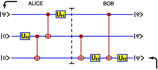
Figure 8: Circuit scheme to teleport an unknown quantum state from Alice to Bob using an arrangement of 3 qubits (coupled quantum dots).

$${\textstyle{1\over 2}}\left\{\left|00\right\rangle(\alpha\left|0\right\rangle+\beta\left|1\right\rangle)+\left|01\right\rangle(\beta\left|0\right\rangle+\alpha\left|1\right\rangle)+\left|10\right\rangle(\alpha\left|0\right\rangle-\beta\left|1\right\rangle)+\left|11\right\rangle(-\beta\left|0\right\rangle+\alpha\left|1\right\rangle)\right\}.$$ (14)

As can be seen from Eq. (14), we are proposing the realization of the Bell basis measurement in two steps [35]: first, we have rotated from the Bell basis into the computational basis $(\left|00\right\rangle$, $\left|01\right\rangle$, $\left|10\right\rangle$, $\left|11\right\rangle)$, by performing the unitary operations shown before the dashed line in Fig. 8. Hence, the second step is to perform a measurement in this computational basis. At this point, we leave QDs a and b in one of the four states $\left|00\right\rangle$, $\left|01\right\rangle$, $\left|10\right\rangle$, $\left|11\right\rangle$ (see Fig. 9(c)), which are the four possible measurement results. This last step can be experimentally realized by using near-field optical spectroscopy [21]. In this way, it is possible to scan, dot-by-dot, the optical properties of the entire dot ensemble, and particularly, to measure directly the excitonic photoluminiscence spectrum of dots $a$ and $b$, thus completing the Bell basis measurement. The result of this measurement provides us with two classical bits of information, conditional the states measured by nanoprobing on QDs a and b (see Fig. 9(c)). These classical bits are essential for completing the teleportation process: rewriting Eq. (14) as

$$\begin{array}[]{c}\frac{1}{2}\left\{\left|00\right\rangle\left|\Psi\right\rangle+\left|01\right\rangle\sigma_{x}\left|\Psi\right\rangle+\right.\left.\left|10\right\rangle\sigma_{z}\left|\Psi\right\rangle+\left|11\right\rangle(-i\sigma_{y})\left|\Psi\right\rangle\right\}\end{array}$$ (15)

we see that if, instead of performing the set of operations shown after the dashed line in Fig. 8, Bob performs one of the conditional unitary operations $I,\sigma_{x},\sigma_{z}$, or $-i\sigma_{y}$ over the QD $c$ (depending on the measurement results or classical signal communicated from Alice to Bob, as shown in Fig. 9(c)) the teleportation process is finished since the excitonic state $\left|\Psi\right\rangle$ has been teleported from dot $a$ to dot $c$. For this reason only two unitary exclusive-or transformations are needed in order to teleport the state $\left|\Psi\right\rangle$. This final step can be verified by measuring directly the excitonic luminescence from dot $c$, which must correspond to the initial state of dot $a$. For instance, if the state to be teleported is $\left|\Psi\right\rangle\equiv\left|1\right\rangle$, the final measurement of the near-field luminiscence spectrum of dot $c$ must give an excitonic emission line of the same wavelength and intensity as the initial one for dot $a$. This measurement process, used for verifying the fidelity of the process, can be used if we either perform the unitary transformations after Alice’s measurement (Fig. 9(c)) or we realize the complete teleportation circuit shown in Fig. 8, leaving the system in the state shown in Fig. 9(d).

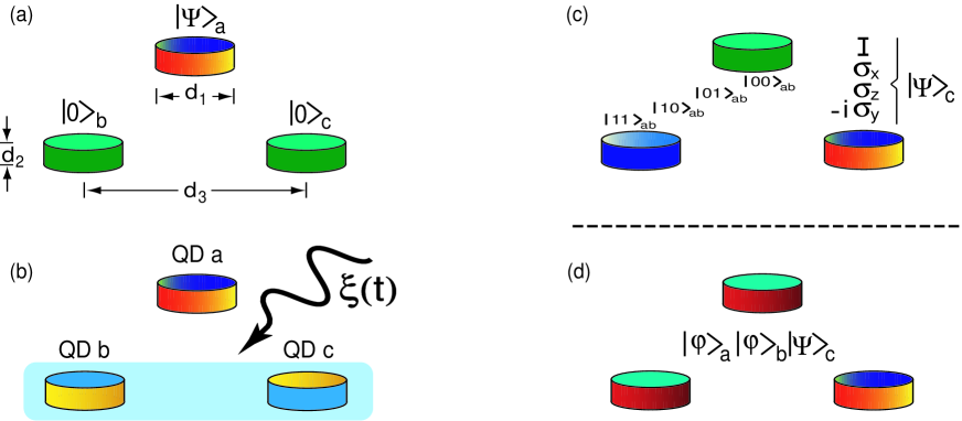
Figure 9: Practical implementation of teleportation using optically-driven coupled quantum dots. (a) Initial state of the system. (b) Intermediate step: radiating the system with the pulse $\xi(t)$. (c) Bell basis measurement and the quantum state of the system at the dashed line in Fig. 8. (d) Final state. Typical values for the dots are diameter $d_{1}=30$ nm, thickness $d_{2}=3$ nm and separation $d_{3}=50$ nm.

As we discussed in Section II, it is possible to excite and probe just one individual QD with the corresponding dephasing time $\tau_{d}=4\times 10^{-11}\;$s [19]. Hence we have the possibility of coherent optical control of the quantum state of a single dot. Furthermore, this mechanism can be extended to include more than one excited state: since ${\displaystyle{\tau_{{}_{Bell}}\over\tau_{d}}}\simeq 1.8\times 10^{-4}$, several thousand unitary operations can in principle be performed in this system before the excited state of the QD decoheres. This fact together with the experimental feasibility of applying the required sequence of laser pulses on the femtosecond time-scale leads us to conclude that we do not need to worry unduly about decoherence ocurring whilst performing the unitary operations that Bob needs in order to obtain the final states schematically sketched in Figs. 9(c) and 9(d), thereby completing the teleportation process. In the case of Fig. 3(a), a similar analysis shows that $\tau_{{}_{GHZ}}=1.3\times 10^{-14}\;$s, and hence$\;{\displaystyle{\tau_{{}_{GHZ}}\over\tau_{d}}}\simeq 3.3\times 10^{-4}$: this also makes the 4 qubits circuit given in Ref. [30] experimentally feasible. Although this discussion refers to ZnSe-based QDs, other regions of parameter space can be explored by employing semiconductors of different bandgap $\epsilon$. As we will discuss in Section 6, we believe that compact hybrid organic-inorganic nanostructures [25] are very promising candidates for the experimental realization of the setup proposed here. In this case, the typical distance between QDs should be of the same order as their size: in ZnSe, the Bohr radius of the three dimensional Wannier exciton $a_{B}\approx 35$A, hence QDs with radii of about 50A will considerably increase the binding energy of these excitons. If these dots are placed in an organic matrix separated by a distance of the same order, we should be able to perform the appropriate quantum operations required in the teleportation process of the excitonic state $\left|\Psi\right\rangle$. Even though the structures that we are considering have a dephasing time of order $10^{-11}$ s, QDs with stronger confinement are expected to have even smaller coupling to phonons giving the possibility for much longer intrinsic coherence times.

In summary, we have proposed a practical implementation of a semiconductor quantum teleportation device, exploiting current levels of optical control in coupled QDs. Furthermore the analysis suggests that several thousand quantum computation operations may in principle be performed before decoherence takes place.

5 Quantum logic with an NMR$-$based nanostructure switch

Here we propose a novel solid-state based mechanism for quantum computation. The essential system is a nuclear spin$-\frac{1}{2}$ impurity placed at the center of a 2 electrons QD in the presence of an external perpendicular magnetic field $B$. These electrons undergo abrupt ground-state transitions as the $B$-field is changed. The different ground states have very different charge distributions and hence different hyperfine interaction with the nucleus. Thus, by changing $B$ we can change the hyperfine coupling and hence tune the nuclear resonance frequency. This allows one to effectively select out one such dot from an array, and the same mechanism may also allow an electron-mediated interaction between nuclei in different dots. The proposal is motivated by recent experimental results which demonstrated the optical detection of an NMR signal in both single QDs [37] and doped bulk semiconductors [38]. Hence the underlying nuclear spins in the QDs can indeed be controlled with optical techniques, via the electron-nucleus coupling. In addition, the experimental results of Ashoori et al. [40] and others, have demonstrated that few electron (i.e. $N\geq 2$) dots can be prepared, and their magic number transitions measured as a function of magnetic field. The requirements for the present proposal are therefore compatible with current experimental capabilities and the complications associated with voltage gates or electron transport of other known proposals (Refs. [12, 13]) are avoided by providing an all-optical system.

5.1 The Model

As we mentioned briefly before, our model considers an array of silicon-based $N-$electron QDs in which impurity atoms (nuclear spin $\frac{1}{2}$) are placed at the center of each QD (see discussion below). Ordinary silicon (²⁸Si) has zero nuclear spin, hence it is possible to construct the QDs such that no nuclear spins are present other than that carried by the impurity nuclei, say ¹³C. Since carbon is an isoelectronic impurity in silicon, no Coulomb field is generated by this impurity. Hence the electronic structure of the bare QDs is essentially unperturbed by the presence of the carbon atom.

Suppose the quantum dots are quasi two-dimensional (2D), contain $N=2$ electrons, and are under the action of the $B$-field. The lateral confining potential in such quasi-2D QDs is typically parabolic to a good approximation: the electrons, with effective mass $m^{\ast}$, are confined by the harmonic potential $\frac{1}{2}m^{\ast}\omega_{0,i}^{2}\mbox{$r$}^{2}$, where $\omega_{0,i}$ is in general different for each dot (see Fig. 10). We consider two configurations in which all of the electrons in the QDs are confined to the (a) $z=0,d,2d,...$ planes (Fig. 10(a)) and (b) $z=0$ plane (Fig. 10(c)). The latter scheme is particularly important because it both facilitates the individual addressability of the qubits and offers a configuration that could be exploited for performing a large number of parallel quantum gates (see Fig. 11). For both of the configurations the repulsion between electrons is modelled by an inverse-square interaction $\alpha r^{-2}$ which leads to the same ground-state physics as a bare Coulomb interaction $r^{-1}$ [41], moreover, such a non-Coulomb form may actually be more realistic due to the presence of image charges [42]. These configurations are considered in such a way that there is not inter-dot tunnelling. In such systems we have two combined effects which are exploited to perform conditional quantum logic gates. First, we have the intra-dot interaction between electrons in the same QD and their coupling to the nuclear qubits. This interaction produces jumps in the relative angular momentum $m$ of the two-electron ground state with increasing $B$. We have shown that these jumps in $m$ cause jumps in the amount of hyperfine splitting in the nuclear spin of the impurity atom, hence providing a switching mechanism for the nuclear-electron spin transitions [36]. Second, we have the correlation between neighbouring dots, i.e. the inter-dot interaction between electrons in different QDs (see Figs. 10(b) and 10(c)). As we will see below, this is the main mechanism responsible for the qubit control given here.

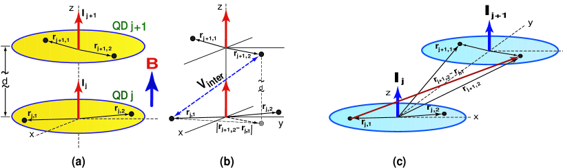
Figure 10: Schematic of the double QD system. Each QD contains 2 electrons. (a) Configuration 1, vertically arranged QDs with the nuclear impurity qubits and the electrons in dots $j$ and $j+1$. (b) Illustration of the inter-dot correlation for electrons $(j+1,2)$, and $(j,1)$. Note that the separation between electrons in different dots is given in terms of the distances $|\mbox{\boldmath$r$}_{i+1,\nu}-\mbox{\boldmath$r$}_{i,\delta}|$ and $d$. The distance $d$ does not correspond with the real scale of the system (see text). (c) Configuration 2, in-plane QDs: schematic of the inter-dot correlation for electrons $(j+1,2)$, and $(j,1)$. In this case, all of the dots are confined to the $z=0$ plane. The dot centers, where the nuclear impurities are located, are separated by a constant distance $d$.

5.2 Hamiltonians and results

Let us analize the theoretical framework for the switching mechanism and the ability to tune the electron-nucleus coupling given here. The Hamiltonian that models the electron spin-nuclear spin dynamics of the single QDs described before, when there is no interaction between them, is given by $H=H_{0}+V$ [36], with

$$H_{0}=H_{2e}+H_{Zeeman},\ \ V=C\mathop{\displaystyle\sum}\limits_{\nu=1}^{2}\mbox{\boldmath$I$}\cdot\mbox{\boldmath$S$}_{\nu}\delta(\mbox{\boldmath$r$}_{\nu})\ \ ,$$ (16)

where $H_{2e}$ includes the orbital degrees of freedom of the two-electron QD in a perpendicular magnetic field and $H_{Zeeman}$ corresponds to the individual electron spins and nuclear spin interaction with the magnetic field. The Fermi contact hyperfine coupling of the nuclear spin with the electron spins is expressed by $V$ in Eq. (16), where the electron-nucleus hyperfine interaction strength is given by $C={\textstyle{8\pi\over 3}}\gamma_{e}\gamma_{n}\hbar^{2}|\phi(z=0)|^{2}$, with $\phi(z=0)$ the single-electron wavefunction evaluated at the QD plane, $\gamma_{e}$ ($\gamma_{n}$) is the electronic (nuclear) gyromagnetic ratio and $\mbox{\boldmath$S$}_{\nu}$ ($I$) is the electron (nuclear) spin. The electron location in the QD plane is denoted by the 2D vector $\mbox{\boldmath$r$}_{\nu}$. Following Ref. [41], $H_{2e}$ splits up into commuting center-of-mass (CM) motion and relative motion ($rel$) contributions, for which exact eigenvalues and eigenvectors can be obtained analytically. The electron-electron interaction only affects the relative motion. The eigenstates of $H$ can be expressed as linear combinations of states labeled as $\left|I_{Z};N,M;n,m;S,S_{Z}\right\rangle$, where $N\;$and $M\;$($n\;$and $m$) are the Landau and angular momentum numbers for the CM (relative motion) coordinates; $S$ and $S_{Z}$ represent the total electron spin and its $z$-component, while $I_{Z}$ represents the $z$-component of the carbon nuclear spin. Consider the two-electron system in its ground state, i.e. $N=M=0$, $n=0$; $m$ determines the orbital symmetry while $S=0,1$ represents the singlet and triplet spin states respectively. Neglecting the off-diagonal orbital coupling terms of the hyperfine interaction $V$, the energy associated with the total Hamiltonian $H$ is $E=E_{CM}+E_{rel}+E_{spin}$, where $E_{CM}$ ($E_{rel}$) denotes the CM ($rel$) electron orbital energy contribution and $E_{spin}$ refers to the eigenvalues of the spin Hamiltonian of the electronic-nuclear system. In the presence of the $B$-field, the low-lying energy levels all have $n=0$ and $m<0$. The relative angular momentum $m$ of the two-electron ground state jumps in value with increasing $B$ (see Refs. [41]). The particular sequence of $m$ values depends on the electron spin because of the overall antisymmetry of the two-electron wavefunction [41]. For example, only odd values of $m$ arise if the $B$-field is sufficiently large for the spin wavefunction to be symmetric (the spatial wavefunction is then antisymmetric). The electron-nucleus coupling depends on the wavefunction value at the nucleus and hence on $m$. The jumps in $m$ will therefore cause jumps in the amount of hyperfine splitting in the nuclear spin of the carbon atom.

The nuclear spin-electron spin effective coupling affecting the resonance frequency $\omega_{{}_{NMR}}$ of the carbon nucleus is given by

$$\Delta(m)={\displaystyle{1\over\pi l^{2}2^{1+\mu_{m}}}}\ \ ,$$ (17)

where $l=\sqrt{\hbar/m^{\ast}\omega}$ is the effective magnetic length, the effective frequency is given by $\omega=\sqrt{\omega_{c}^{2}+4\omega_{0}^{2}}$, $\omega_{c}=eB/m^{\ast}$ is the cyclotron frequency. The term $\mu_{m}=\left(m^{2}+\frac{\alpha/l_{0}^{2}}{\hbar\omega_{0}}\right)^{\frac{1}{2}}$ absorbs the effects of the electron-electron interaction and $l_{0}=\sqrt{\hbar/m^{\ast}\omega_{0}}$ is the oscillator length. Hence, the effective spin Hamiltonian $H_{S}$ has the form

$$H_{S}=A(m)\left[(I_{+}S_{-}+I_{-}S_{+})+2I_{Z}S_{Z}\right]-\gamma_{n}BI_{Z}+\gamma_{e}BS_{Z}\ \ ,$$ (18)

where $A(m)=\frac{1}{2}C\Delta(m)$ represents a $B$-dependent hyperfine coupling. We note that the first term of the hyperfine interaction in Eq. (18) corresponds to the dynamic part responsible for nuclear-electron flip-flop spin transitions while the second term describes the static shift of the electronic and nuclear spin energy levels.

Electrons in the singlet state ($S=0$) are not coupled to the nucleus. In this case, the nuclear resonance frequency is given by the undoped-QD NMR signal $\hbar\omega_{{}_{NMR,0}}=\gamma_{n}B$. For electron triplet states, the nuclear resonance signal corresponds to a transition where the electron spin is unaffected by a radio-frequency excitation pulse whereas the nuclear spin experiences a flip. This occurs for the transition between states $\left|-;1,-1\right\rangle$ and $\left|\Psi\right\rangle=c_{1}\left|+;1,-1\right\rangle+c_{2}\left|-;1,0\right\rangle$. The coefficients $c_{1}$ and $c_{2}$ can be obtained analytically by diagonalizing the Hamiltonian given in Eq. (18). Hence

$$\hbar\omega_{{}_{NMR}}={\textstyle{3\over 2}}{\displaystyle{A(m)}+{\textstyle{1\over 2}}\left(\gamma_{n}-\gamma_{e}\right)B}+{\textstyle{1\over 2}}\left[\left[\displaystyle{A(m)}+\left(\gamma_{n}+\gamma_{e}\right)B\right]^{2}+8A^{2}(m)\right]^{\frac{1}{2}}.$$ (19)

Since $\gamma_{e}>>\gamma_{n}$, $\hbar\omega_{{}_{NMR}}\approx\gamma_{n}B+2A(m)$ which illustrates the dependence of the NMR signal on the effective $B$-dependent hyperfine interaction.

Figure 11(a) shows the effective coupling $\Delta(m)$ between the two-electron gas and nucleus as a function of the ratio between the cyclotron frequency and the harmonic oscillator frequency. (The CM is in its ground state). For silicon, $C/l_{0}^{2}=60$ MHz. For $B$-field values where the electron ground state is a spin singlet ($m$ even) no coupling is present. The strength of the effective coupling decreases as the $B$-field increases due to the larger spatial extension of the relative wavefunction at higher $m$ values, i.e. the electron density at the centre of the dot becomes smaller. The $B$-field provides a very sensitive control parameter for controlling the electron-nucleus effective interaction. In particular, we note the large abrupt variation of $\Delta(m)$ for $\frac{\omega_{c}}{\omega_{0}}\approx 2.1$ where the electron ground state is performing a transition from a spin triplet state ($m=1$) to a spin triplet state ($m=3$). This ability to tune the electron-nucleus coupling underlies the present proposal for an NMR-based switch.

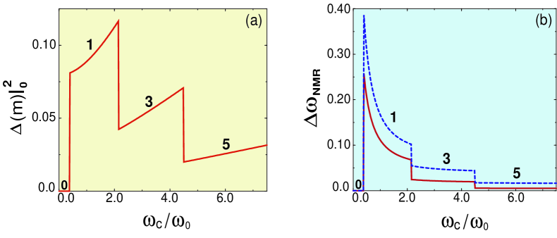
Figure 11: (a) Variation of the electron spin$-$nucleus spin effective coupling $\Delta(m)$ as a function of $\frac{\omega_{c}}{\omega_{0}}$. The center-of-mass motion remains in its ground state. The electron repulsion strength is given by $\frac{\alpha/l_{0}^{2}}{\hbar\omega_{0}}=3.0$. The sequence of transitions is given by $(|m|,S)=\{(0,0),(1,1),(3,1),(5,1),...\}$. (b) Relative variation of the effective nuclear magnetic resonance frequency of the carbon impurity nucleus. $\frac{\alpha/l_{0}^{2}}{\hbar\omega_{0}}=3.0$. Solid line corresponds to center-of-mass in the ground state. Dashed line corresponds to center-of-mass in the first excited state after absorption of IR light.

We also give an additional method for externally controlling the nucleus-electron effective coupling using optics [36]: in the presence of infra-red (IR) radiation incident on the QD, the CM wavefunction will be altered since the CM motion absorbs IR radiation. (The relative motion remains unaffected in accordance with Kohn’s theorem). By considering the CM transition from the ground state $\left|N=0,M=0\right\rangle$ to the excited state $\left|N=1,M=1\right\rangle$, which becomes the strongest transition in high $B$-fields, we get the new spin-spin coupling term given by

$$\Delta_{{}_{CM}}(m)=\left({\displaystyle{1+\mu_{m}\over 2}}\right)\Delta(m)\ \ .$$ (20)

Hence the nuclear spin-electron spin coupling is renormalized by the factor ${\textstyle{1+\mu_{m}\over 2}}$ in the presence of IR radiation. Figure 11(b) shows the relative variation of $\omega_{{}_{NMR}}$ with respect to the undoped QD NMR signal, i.e. $\Delta\omega_{{}_{NMR}}=\frac{\omega_{NMR}-\omega_{NMR,0}}{\omega_{NMR,0}}$ (solid line) as a function of the frequency ratio $\frac{\omega_{c}}{\omega_{0}}$. The jumps in the carbon nucleus resonance are abrupt, reaching 25% in the absence of IR radiation. This allows a rapid tuning on and off resonance of an incident radio-frequency pulse. The NMR signal in regions of spin-singlet states remains unaltered. Moreover, the nuclear spin is being controlled by radio-frequency pulses which are externally imposed, thereby offering a significant advantage over schemes which need to fabricate and control electrostatic gates near to the qubits, such as Refs. [12, 13]. Illuminating the QD with IR light will shift the frequencies $\omega_{{}_{NMR}}$ (see dashed line in Fig. 11(b)) hence providing further all-optical control of the nuclear qubit. A crucial aspect of the present proposal is the capability to manipulate individual nuclear spins. All-optical NMR measurements in semiconductor nanostructures [37, 38] together with local optical probe experiments are quickly approaching such a level of finesse.

Next, let us consider the situation of a system of $K$ dots which interact with each other: the new Hamiltonian associated with this configuration (see Fig. 10) is $H=H_{0}+V$, with

$$H_{0}=\mathop{\displaystyle\sum}\limits_{i=1}^{K}\Big{(}H_{2e}^{(i)}-\gamma_{n}BI_{i}^{z}+\mathop{\displaystyle\sum}\limits_{\nu=1}^{2}\gamma_{e}BS_{i,\nu}^{z}\Big{)},\ \ V=C\mathop{\displaystyle\sum}\limits_{i=1}^{K}\mathop{\displaystyle\sum}\limits_{\nu=1}^{2}\mbox{\boldmath$I$}_{i}\cdot\mbox{\boldmath$S$}_{i,\nu}\delta(\mbox{\boldmath$r$}_{i,\nu})+V_{inter}\ \ ,$$ (21)

where $\mbox{\boldmath$S$}_{i,\nu}$ ($\mbox{\boldmath$I$}_{i}$) is the spin polarization of electron $\nu$ (nucleus) in dot $i$. The location of electron $\nu$ in the $i-$th QD is denoted by $\mbox{\boldmath$r$}_{i,\nu}$. The first term in Eq. (21) represents the $i-$th two-electron QD with a perpendicular $B$-field, which includes the intra-dot interaction ($V_{intra}$), while the others give the nuclear and the electron-spin Zeeman energies in dot $i$ ($z$ indicates the component of these spin operators). The second term of Eq. (21) give the Fermi contact hyperfine coupling of the nuclear spin of dot $i$ with the electron spin $\nu$ in the same dot and $V_{inter}$ represents the inter-dot interaction between electrons in neighbouring QDs. The nuclear spin control is performed by the inter-dot coupling $V_{inter}$ due to the interaction between electrons in neighbouring dots. This mechanism (rather than the direct dipole-dipole interaction between the nuclei) is the responsible for the qubit control in the present proposal. In the case of configuration 1 (Fig. 10(a)), we have

$$V_{inter}^{(1)}=\mathop{\displaystyle\sum}\limits_{i=1}^{K}\ \mathop{\displaystyle\sum}\limits_{\nu,\delta=1}^{2}\frac{\alpha}{|\mbox{\boldmath$r$}_{i+1,\nu}-\mbox{\boldmath$r$}_{i,\delta}|^{2}+d^{2}}\ \ ,$$ (22)

where $\mbox{\boldmath$r$}_{i+1,\nu}-\mbox{\boldmath$r$}_{i,\delta}\equiv\left([\mbox{$r$}_{i+1,\nu}-\mbox{$r$}_{i,\delta}]_{{}_{x}},[\mbox{$r$}_{i+1,\nu}-\mbox{$r$}_{i,\delta}]_{{}_{y}}\right)$. We will assume that the separation between neighbouring QDs is such that ${|\mbox{\boldmath$r$}_{i+1,\nu}-\mbox{\boldmath$r$}_{i,\delta}|^{2}<d^{2}}$. This means that the square of the $xy-$plane separation between electrons in neighbouring dots (see Fig. 10(b) for the case of electrons $(j+1,2)$, and $(j,1)$) is less than the square of the vertical separation between such dots ($d^{2}$), as illustrated in Fig. 10(b). Hence, the minimum value for $d$ is determined by the largest $xy-$projection of electrons in neighbouring dots, which roughly corresponds to the sum of the radii of such dots. The case of configuration 2 (Figs. 10(c) and 11) has

$$V^{(2)}_{inter}=\mathop{\displaystyle\sum}\limits_{i=1}^{K}\ \mathop{\displaystyle\sum}\limits_{\nu,\delta=1}^{2}\frac{\alpha}{|\mbox{\boldmath$r$}_{i+1,\nu}-\mbox{\boldmath$r$}_{i,\delta}|^{2}}\ \ ,$$ (23)

where the in-plane vectors $\mbox{\boldmath$r$}_{i,\epsilon}$ are defined as above.

5.2.1 Single-qubit rotations

Single qubit rotations, e.g. the Hadamard transformation $U_{H}$, can be performed by rotating the single nuclear qubit of resonant frequency $\omega_{i}$ via the application of RF pulses at the appropriate frequency for a given duration and amplitude of the $B$-field. The coherence time of the nuclear spins is estimated by measuring their $T_{1}$ and $T_{2}$ relaxation times, i.e. their nuclear spin-flip relaxation times and the rate of loss of phase coherence between the qubits respectively. In the silicon-based nanostructures considered here, $T_{1}$ can be estimated in the 1$-$10 hour range [44] (for $T<4$ K and $B<1$ T). In isotopically purified ²⁸Si, Si:P linewidths are $<1$ MHz, which gives for $T_{2}$ times greater than 0.5 ms [12]. In our case, the electrostatically neutral character of the impurity atom ¹³C (and the fact that the silicon nuclei surrounding it have no nuclear spin) makes the carbon nuclear spin state very effectively shielded from the environment and hence we would expect to have far longer $T_{2}$ times than the (charged) donor nuclei mentioned above.

5.2.2 The C$-$NOT gate

The inter-dot interaction potentials given by Eqns. (22) and (23) produce the necessary nuclear qubit coupling for reliable implementation of the two-qubit gates required for quantum computation. In doing so, the Hamiltonian $H$ has $K=2$ and conditional quantum dynamics can be performed based on the selective driving of spin resonances of the two impurity nuclear qubits, say $I_{1}$, and $I_{2}$, in this system of two coupled QDs (see Fig. 10). The interaction potentials are given by

$$V_{inter}^{(1)}=\mathop{\displaystyle\sum}\limits_{\nu,\delta=1}^{2}\frac{\alpha}{|\mbox{\boldmath$r$}_{2,\nu}-\mbox{\boldmath$r$}_{1,\delta}|^{2}+d^{2}}\ \ ,\ \ V^{(2)}_{inter}=\mathop{\displaystyle\sum}\limits_{\nu,\delta=1}^{2}\frac{\alpha}{|\mbox{\boldmath$r$}_{2,\nu}-\mbox{\boldmath$r$}_{1,\delta}|^{2}}\ \ .$$ (24)

In these schemes, the orthonormal computation basis of single qubits $\left\{\left|0\right\rangle,\left|1\right\rangle\right\}$ is represented by the spin down and up of the impurity nuclei. The QDs do not need to be identical in size. The coupling between QDs gives an additional magic number transition as a function of $B$-field which can be used for selective switching between dots, i.e. since the ground state switches back and forth between product states and entangled states [43], the resonant frequency for transitions between the states $\left|0\right\rangle,$ and $\left|1\right\rangle$ of one nuclear spin (target qubit) depends on the state of the other one (control qubit). In this way, such coupled QDs can be used to generate the conditional C-NOT gate. The quantum computing scheme proposed here could be easily scalable to large quantum information processors: QDs would be individually addressed via the action of an appropriate $B$-field. This is shown in Fig. 12, where the $B_{j,j+1}$ field is assumed to be locally addressing the qubits $j$ and $j+1$ from the entire ensemble of dots. Even if the QD array is irregular, one may still be able to perform the solid-state equivalent of the bulk/ensemble NMR computing recently reported in Ref. [45]. The coupling of the qubits to an external reservoir and the task of controlling the quantum coherence of the proposed system are currently being addressed [43]. However, and as we discussed below, due to the exceptionally low decoherence rates of these nuclear qubits, the required RF pulses would allow us to perform a sufficient number of single qubit rotations and two-qubit gates for realizing “useful” quantum computing tasks (e.g. the Grover algorithm) before the system decoheres.

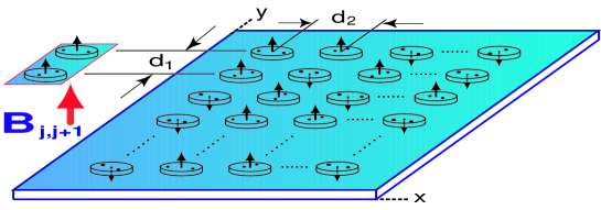
Figure 12: Scaling up Configuration 2 (See Fig. 10 (c)): The $K$ dots of the system are confined to the $z=0$ plane. Within the entire ensemble of dots, the $B$-field is able to locally address: (a) single QDs, as in the case of one qubit rotations and (b) double dots (e.g. the $j$ and $j+1$ dots in the figure) as required in the case of two-qubit logic gates. The dot centers, where the nuclear impurities are located, are separated by constant distances $d_{1}$ and $d_{2}$.

6 Concluding remarks

We would like to highlight some aspects of the choice of materials and experimental parameters for the implementation of the systems considered here. Regarding the experimental requirements for building the excitonic setup proposed in Section 2 we point out that hybrid organic-inorganic nanostructures would be very good candidates [25] since they provide us with large radius (Wannier-Mott) exciton states in the inorganic material and small-radius (Frenkel) exciton states in the organic one. Hence the hybrid material will be characterized by a radius dominated by their Wannier component and by an oscillator strength dominated by their Frenkel component. This means that the desirable properties of both the organic and the inorganic material are brought together to overcome basic limitations which arise if each one acts separately. Following recent results [25], if we consider a system of two or three QDs (as required in the present proposal) of an inorganic II-VI material (e.g. the extensively studied ZnSe or ZnCdSe), embedded in bulk-like organic crystalline material (e.g. tetracene, perylene, fullerene, PTCDA) where their Frenkel and Wannier excitons are in resonance with each other, we would expect a strong hybridization between these excitons, which means a greater Wannier exciton delocalization or Förster hopping. To achieve this, the typical distance between QDs should be of the same order as their size: In ZnSe, the Bohr radius of the three dimensional Wannier exciton $a_{B}\approx 35$A, hence QDs with radii of about 50A will considerably increase the binding energy of these excitons. If these dots are placed in an organic matrix (as discussed above) separated by a distance of the same order, we should be able to observe the entangled states proposed here. There has recently being an experimental observation of photon antibunching from an artificial atom (a single CdSe/ZnS quantum dot) [39], i.e. the detection of quantum correlations among photons from a single quantum dot. We note that the statistical properties of resonance fluorescence from the ensemble of QDs proposed in Section 2 should likewise give raise to a signature associated with excitonic state entanglement. Theoretical details of this multi-dot excitonic signature will be reported elsewhere [29].

Regarding the NMR setup of the above section, there may be a natural way to make a quantum dot in silicon with a single C atom inside it. C atoms are known to act as nucleation centers for SiGe quantum dots (see e.g. Ref. [47]). Another possibility would be to consider an isolated ²⁹Si (spin 1/2 and natural abundance 4.7%) at the center of a ²⁸Si based QD. The isoelectronic character of the impurity is reinforced but possible purification procedures could be harder to implement. The more realistic situation of a non-centered impurity, i.e. when the impurity atom is away from the QD center, will modify the discontinuity strengths of the electron-nucleus coupling since this coupling is affected by the density of probability of the CM wavefunction at the impurity site [36]; however the main effects discussed in the present proposal remain the same. For a typical $N=2$ electrons QD with 30 $n$m of diameter, lateral confining potential $\omega_{0}=8.2\times 10^{12}$ s^-1 ($\hbar\omega_{0}=5.4$ $m$eV), and low temperatures ($T<$ 1 K) [40], we would expect a singlet-triplet transition $(m,S)=(0,0)\mapsto(1,1)$ at $B\approx 1.3$ T, or the triplet-triplet transition $(1,1)\mapsto(3,1)$ at $B\approx 6.4$ T. If the harmonic potential is such that $\hbar\omega_{0}=1.1$ $m$eV (see Ref. [40]) the above transitions would be expected at $B$-fields of 0.3 T and 1.4 T, respectively. For this system, we can estimate the lower limit of the “gating time” $\tau_{g}$, i.e. the time for the execution of an individual quantum gate: since the energy splitting of the two nuclear qubits, i.e. the value of the energy difference between the next excited state and the ground singlet and triplet states of our two-electron system $\Delta E\sim 0.3$ $m$eV, the lower limit of $\tau_{g}$ is

$$\tau_{g}\gg{\textstyle{\hbar\over\Delta E}}\sim 1\ {\rm ps}\,.$$ (25)

Therefore, as long as the gating time $\tau_{g}$ is longer than, say, 0.1 $n$s, the QD is well isolated, so that the higher excited states can be safely neglected, and the gating action can be considered adiabatic. The number of elementary operations that could in principle be performed on a single nuclear qubit before it decoheres is ${\textstyle{\tau_{dec}\over\tau_{g}}}\approx 10^{9}$. This figure of merit should be more than enough to satisfy the current criteria for quantum error correction schemes since fault-tolerant quantum computation has been shown to be successful if the decoherence time is $10^{4}-10^{5}$ times the gating time. Finally, there is the important issue of the spin measurements that have to be implemented for either the input or the readout of single spin qubits. This process must be rapid enough to avoid decoherence of the qubits: optical NMR techniques for reading the input/output of these spin states are currently approaching such a level of finesse [37, 38]. Other mechanisms for measuring these spin states are also currently under intensive experimental study [46].

The solid state NMR proposal given here is not in principle limited to $N=2$ electrons: generalizations [48] of the present angular momentum transitions arise for $N>2$. It was pointed out recently [49] that the spin configurations in many-electron QDs could be explained in terms of just two-electron singlet and triplet states. Therefore, the present results may occur in QDs with $N>2$.

It is worth noting that our proposal is not based upon the possibility of applying a localized magnetic field to a single quantum dot. The procedure to switch the NMR frequency of a single nuclear spin is based upon the magic number transitions which can be implemented by an extended magnetic field. It is the local hyperfine electron-nucleus coupling within each quantum dot which can be tuned by such magic number transitions. This is the main point of our proposal: the control of the local hyperfine coupling by an extended magnetic field may be used to perform single nuclear spin manipulation as well as the solid-state equivalent of the bulk/ensemble liquid NMR computing (see Ref. [45]), for an array of either identical or non-indentical quantum dots. Similar to the NMR liquid experiments, the quantum dot NMR resonance is determined by local effects: in our case these are dominated by electron ground-state transitions. At the present, there is a tremendous motivation to perform the setup proposed in our work: first, Rabi oscillations have not yet been experimentally demonstrated in QDs, and we believe that our setup offers an excellent opportunity for doing so. As discussed, the ground state energies of QDs with $N$ electrons in the presence of magnetic fields, the ones required for our proposal, have already been experimentally studied (see e.g. Refs. [40, 49]). Second, there is the possibility of performing quantum logic gates with very low decoherence rates. We also would like to note that the magic number transitions considered here require a relaxation process of the electron system to achieve the new ground state, i.e. the changes in the $B$-field (which change the hyperfine coupling and hence tune the nuclear resonance frequency) must be done $adiabatically$ to be able to perform the jumps in the angular momentum quantum number. This electron relaxation is compatible with the requirement of maintaining the quantum coherence due to the fact that information is stored in the nuclear spin qubit. It is well known that the nuclear spin relaxation times are several orders of magnitude longer than electron relaxation times. Therefore, electrons in the quantum dot can evolve to a new ground state before any environmentally-induced contamination affects the nuclear spin state.

To summarize, we have shown that semiconductor nanostructures can be exploited in order to realize all-optical quantum entanglement schemes, even in the presence of noisy environments. A scheme for quantum teleportation of excitonic states has also been proposed. In addition, we have presented a solid state NMR-based mechanism for performing reliable quantum computation.

Acknowledgements. The authors acknowledge the suppport of the Colombian government agency for science and technology, COLCIENCIAS.

References

- [1] See the articles in March 1998 issue of Physics World.
- [2] P.W. Shor, in Proceedings of the 35th Annual Symposium on the Foundations of Computer Science, ed. by S. Goldwasser (IEEE Computer Society, Santa Fe, Los Alamitos, CA), 124 (1994).
- [3] J.I. Cirac and P. Zoller, Phys. Rev. Lett. 74, 4091 (1995); Nature 404, 579 (2000); C. Monroe, D.M. Meekhof, B.E. King, W.M. Itano, and D.J. Wineland, ibid. 75, 4714 (1995); K. Molmer and A. Sorensen, Phys. Rev. Lett. 82, 1835 (1999) (see also Pre-print quant-ph/0002024); C.A. Sackett et al., Nature 393, 133 (2000).
- [4] Q.A. Turchete, C.J. Hood, W. Lange, H. Mabuchi, and H.J. Kimble, Phys. Rev. Lett. 75, 4710 (1995).
- [5] N.A. Gershenfeld and I.L. Chuang, Science 275, 350 (1997); D.G. Cory, A.F. Fahmy, and T.F. Havel, Proc. Natn. Acad. Sci. USA 94, 1634 (1997); E. Knill, I.L. Chuang, and R. Laflamme, Phys. Rev. A 57, 3348 (1998); J.A. Jones, M. Mosca, and R.H. Hansen, Nature 393, 344 (1998).
- [6] A. Shnirman, G. Schön, and Z. Hermon, Phys. Rev. Lett. 79, 2371 (1997); D.V. Averin, Solid State Commun. 105, 659 (1998); Y. Makhlin, G. Schön, and A. Shnirman, Nature 398, 305 (1999).
- [7] B.E. Kane, Nature 393, 133 (1998); D. Loss, and D.P. DiVincenzo, Phys. Rev. A 57, 120 (1998); G. Burkard, D. Loss, and D.P. DiVincenzo, Phys. Rev. B 59, 2070 (1999); A. Barenco et al., Phys. Rev. Lett. 74, 4083 (1995); A. Imamoglu et al., Phys. Rev. Lett. 83, 4204 (1999); R. Vrijen et al., Phys. Rev. A 62, 12306 (2000).
- [8] D.M. Greenberger, M.A. Horne, A. Shimony and A. Zeilinger, Am. J. Phys. 58, 1131 (1990).
- [9] N.F. Johnson, J. Phys.: Condens. Matt. 7, 965 (1995).
- [10] I.L. Chuang, L.M.K. Vandersypen, X. Zhou, D.W. Leung, and S. Lloyd, Nature 393, 143 (1998); J.A. Jones and M. Mosca, J. Chem. Phys. 109, 1648 (1998).
- [11] I.L. Chuang, N. Gershenfeld, and M. Kubinec, Phys. Rev. Lett. 80, 3408 (1998); J.A. Jones, M. Mosca, and R.H. Hansen, Nature 393, 344 (1998).
- [12] B.E. Kane, Nature 393, 133 (1998).
- [13] V. Privman, L.D. Vagner, and G. Kventsel, Phys. Lett. A 239, 141 (1998).
- [14] K. Obermayer, W.G. Teich, and G. Mahler, Phys. Rev. B 37, 8111 (1988).
- [15] N.H. Bonadeo, G. Chen, D. Gammon, D.S. Katzer, D. Park, and D.G. Steel, Phys. Rev. Lett. 81, 2759 (1998).
- [16] X. Hu and K. Schulten, Physics Today, August (1997), p. 28.
- [17] A. Aspect et al., Phys. Rev. Lett. 49, 91 (1982); P. Kwiat et al., Phys. Rev. Lett. 75, 4337 (1995); D. Bowmeester et al., Nature 390, 575 (1997).
- [18] I.L. Chuang et al., Proc. R. Soc. Lond. A 454, 447 (1998).
- [19] N.H. Bonadeo, J. Erland, D. Gammon, D.S. Katzer, D. Park, and D.G. Steel, Science 282, 1473 (1998).
- [20] G. Bartels et al., Phys. Rev. Lett. 81, 5880 (1998).
- [21] A. Chavez-Pirson, J. Temmyo, H. Kamada, H. Gotoh, and H. Ando, Appl. Phys. Lett. 72, 3494 (1998).
- [22] J.H. Reina, L. Quiroga, and N.F. Johnson, Phys. Rev. A 62, 12305 (2000); L. Quiroga and N.F. Johnson, Phys. Rev. Lett. 83, 2270 (1999).
- [23] A. Wokaun and R.R. Ernst, J. Chem. Phys. 67, 1752 (1977).
- [24] S. Vega, J. Chem. Phys. 68, 5518 (1978).
- [25] For a review, see V.M. Agranovich et al., J.Phys.: Condens. Matter 10, 9369 (1998) and references therein.
- [26] T. Takagahara, Phys. Rev. B 60, 2638 (1999).
- [27] F.J. Rodríguez, L. Quiroga, and N.F. Johnson, Physica Status Solidi (a) 178, 403 (2000).
- [28] N. Bogolubov Jr. et al., Physica A 151, 293 (1988).
- [29] L. Quiroga, J.H. Reina, and N.F. Johnson, in preparation.
- [30] J.H. Reina and N.F. Johnson, Phys. Rev. A, to be published. See e-print cond-mat/9906034.
- [31] C.H. Bennett, G. Brassard, C. Crépeau, R. Jozsa, A. Peres, and W.K. Wooters, Phys. Rev. Lett. 70, 1895 (1993).
- [32] D. Bowmeester, J.W. Pan, K. Mattle, M. Eibl, H. Weinfurter, and A. Zeilinger, Nature 390, 575 (1997); D. Boschi, S. Branca, F. De Martini, L. Hardy, and S. Popescu, Phys. Rev. Lett., 80, 1121 (1998); A. Furusawa, J.L. Sorensen, S.L. Braunstein, C.A. Fuchs, H.J. Kimble, and E.S. Polzik, Science 282, 706 (1998); M.A. Nielsen, E. Knill, and R. Laflamme, quant-ph/9811020.
- [33] A. Einstein, B. Podolsky, and N. Rosen, Phys. Rev. 47, 777 (1935).
- [34] S.L. Braunstein, A. Mann, and M. Revzen, Phys. Rev. Lett. 68, 3259 (1992).
- [35] G. Brassard, S.L. Braunstein, and R. Cleve, Physica D 120, 43 (1998).
- [36] J.H. Reina, L. Quiroga, and N.F. Johnson, Phys. Rev. B (rapid comm.) 62, 2267 (2000).
- [37] S.W. Brown, T.A. Kennedy, and D. Gammon, Solid State Nuclear Mag. Res. 11, 49 (1998).
- [38] J.M. Kikkawa and D.D. Awschalom, Science 287, 473 (2000).
- [39] P. Michler et al., Nature 406, 968 (2000).
- [40] R.C. Ashoori, H.L. Stormer, J.S. Weiner, L.N. Pfeiffer, K.W. Baldwin, and K.W. West, Phys. Rev. Lett. 71, 613 (1993).
- [41] L. Quiroga, D.R. Ardila, and N.F. Johnson, Solid State Commun. 86, 775 (1993); M. Wagner , U. Merkt, and A.V. Chaplik, Phys. Rev. B 45, 1951 (1992).
- [42] L.D. Hallam, J. Weis, and P.A. Maksym, Phys. Rev. B 53, 1452 (1996).
- [43] J.H. Reina, L. Quiroga, and N.F. Johnson, in preparation.
- [44] G. Feher, Phys. Rev. 114, 1219 (1959); D.K. Wilson and G. Feher, Phys. Rev. 124, 1068 (1961).
- [45] N.A. Gershenfeld and I.L. Chuang, Science 275, 350 (1997); D.G. Cory, A.F. Fahmy, and T.F. Havel, Proc. Natl. Acad. Sci. USA 94, 1634 (1997).
- [46] B. Kane, e-print quant-ph/0003031; R. Vrijen et al., Phys. Rev. A 62, 12306 (2000) and references therein.
- [47] O.G. Schmidt, S. Schieker, K. Eberl, O. Kienzle, and S. Ernst, App. Phys. Lett. 73, 659 (1998).
- [48] P.A. Maksym and T. Chakraborty, Phys. Rev. Lett. 65, 108 (1990); N.F. Johnson and L. Quiroga, ibid. 74, 4277 (1995).
- [49] S. Tarucha, D.G. Austing, Y. Tokura, W.G. van der Wiel, and L.P. Kouwenhoven, Phys. Rev. Lett. 84, 2485 (2000).