NMR Quantum Computation

I Introduction

Quantum computation Bennett:2000 ; Macchiavello:2000 ; Bouwmeester:2000 offers the prospect of revolutionising many areas of science by allowing us to solve problems well beyond the power of our current classical computers Shor:1999 . In particular a quantum computer would be superb for simulating the behaviour of other complex quantum mechanical systems Feynman:1982 ; Lloyd:1996 . Although the theory of quantum computation has been studied for many years, and many important theoretical results have been obtained, early attempts to actually build even the smallest quantum computer proved extremely challenging.

In recent years there has been considerable interest in the use of NMR techniques Ernst:1987 to implement quantum computations Cory:1996 ; Cory:1997 ; Gershenfeld:1997 ; Jones:1998a ; Chuang:1998a ; Jones:2000b ; Jones:2000c . It has proved surprisingly simple to build small NMR quantum computers, and while such computers are themselves too small for any practical use, their mere existence has brought great excitement to a field largely deprived of experimental achievements.

I.1 Structure and scope

In this article I will describe how NMR techniques may be used to build simple quantum information processing devices, such as small quantum computers, and show how these techniques are related to more conventional NMR experiments. Many tricks and techniques well known from conventional NMR studies can be applied to NMR quantum computation, and it is likely that some of these will be applied in any large scale quantum computer which is eventually built. Conversely, techniques from quantum computation could have applications within NMR.

It is impossible to explain how NMR may be used to implement quantum computations without first explaining what quantum computation is, and what it could achieve. This in turn requires a brief discussion of classical reversible computation Feynman:1996 . In order to reduce these introductory sections to a reasonable length many technical points have inevitably been skipped over. Wherever possible I will use traditional product operator notation Sorensen:1983 to describe how NMR quantum computers are implemented; it will sometimes, however, be necessary to use more abstract quantum mechanical notations Goldman:1988 to describe what these computers seek to achieve.

Before the advent of NMR quantum computation, almost all research in this field was performed within a small community of physicists and mathematicians. Some important results have never been published as conventional papers, but simply circulate as electronic preprints; copies of most of these can be obtained from the quant-ph archive on the LANL e-print server LANL . Similarly, many other papers appear as LANL e-prints long before more formal publication.

II Limits to computation

Over the last forty years there has been astonishing progress in the power of computational devices using silicon based integrated circuits. This progress is summarised in a set of “laws”, usually ascribed to Moore, although some were developed by other people. Over this period the power of computational devices has roughly doubled every eighteen months, or increased ten fold every five years. Unfortunately, this extraordinary technological progress may not continue for much longer, as this increase in computing power requires a corresponding decrease in the size of the transistors on the chip; this shrinking process cannot be continued indefinitely as the transistors will eventually be reduced to the atomic scale. At current rates of progress it is estimated Schulz:1999 that the ultimate limits of this approach will be reached by about 2012, and any further progress in the power of our computers will require a radically different approach. One possible approach is to use the power offered by quantum computation.

II.1 Computational complexity

Even if the problems described above are sidestepped in some way, there are still strong limits to the problems which we can solve with current computers. These limits are derived from the underlying theory of computation itself, and in particular from computational complexity theory Welsh:1988 . Complexity theory considers the classification of mathematical problems according to how difficult they are to deal with, and seeks to divide them into those which are relatively easy (tractable) and those which are uncomfortably difficult (intractable). Note that complexity theory is not concerned with problems which we do not know how to solve, or which we know cannot be solved, but only with problems for which an algorithmic solution (tractable or intractable) is known.

The classical theory of computation has remained largely unchanged for decades, with a central role played by the Church–Turing thesis. This asserts that all physically reasonable models of computation are ultimately equivalent to one another, so that it is not really necessary to consider any particular computer when assessing the complexity of a problem; any reasonable model will do. In particular, the tractability or otherwise of a problem is independent of the computational device used. As we will see, quantum computation challenges this thesis, as quantum computers appear to be fundamentally more powerful than their classical equivalents.

To make further progress it is necessary to use a more precise measure of the complexity of an algorithm. The usual approach is to determine the computational resources (most commonly defined as the number of elementary computational operations) required to implement it. Clearly this measure will depend on the exact nature of the computational resources available to our computer, and so this is not directly useful. A better approach is to consider not a single isolated problem, but a family of closely related problems, and to determine how the resources required scale within this family. To take a simple example, adding two $n$ digit numbers with pencil and paper requires $n$ separate additions, together with $n$ carries, and so the time required for addition scales linearly with $n$. Similarly, multiplying two $n$ digit numbers by long multiplication requires $n^{2}$ multiplications and a similar number of additions.

Mathematically, adding two $n$ digit numbers is said to be $O(n)$ (that is, of order $n$). The exact number of steps required will depend on exactly how elementary computational steps are counted, but the total number of steps will always scale linearly with $n$. Similarly, long multiplication can always be performed in a number of steps which varies quadratically with $n$, and so is $O(n^{2})$.

The complexity of a problem, rather than an algorithm, may be defined as the complexity of the best known algorithm for solving the problem; thus addition is $O(n)$. It might seem that multiplication is $O(n^{2})$, but in fact long multiplication is not the best known algorithm; a better approach is known with complexity about $O(n\log n)$ Welsh:1988 . Strictly speaking one should also distinguish between an upper bound on the number of steps known to be sufficient to solve a problem (indicated by $O$), and a lower bound on the number of steps known to be required to solve a problem (indicated by $\Omega$); a problem, such as addition of $n$ digit numbers, which is both $O(n)$ and $\Omega(n)$ is denoted as $\Theta(n)$.

Problems, such as addition and multiplication, whose complexity is at worst a polynomial function of $n$, are said to be easy, while problems whose complexity is worse than a polynomial function of $n$ are said to be hard. For example, consider the problem of finding the prime factors of an $n$ digit composite number. The obvious way to do this is to simply try dividing the composite number by every number less than its square root; as there are approximately $\sqrt{10^{n}}=10^{n/2}$ such trial divisors, this algorithm has complexity $O(10^{n/2})$. Better algorithms for factoring are known, but they all have the same property of exponential complexity.

For problems with polynomial complexity, especially those whose complexity is described by a low power of $n$, such as $n$ or $n^{2}$, the effort required to solve a problem increases only slowly with $n$. Thus it should be possible to tackle such problems for a reasonable range of input sizes, and a modest increase in computer power should give a significant increase in this range. Exponential functions, however, rise extremely rapidly with $n$, and so it will only be possible to solve problems with exponential complexity for relatively small input sizes; furthermore a modest increase in computer power will result in only a tiny increase in the range of problems that can be solved.

The apparent exponential complexity of factoring is a matter of some importance, as it underlies many cryptographic schemes in use today, notably those based on the Rivest–Shamir–Adleman (RSA) approach to public key cryptography, such as PGP (Pretty Good Privacy) Schneier:1996 . These schemes involve a public key, which anyone may use to encrypt a message, and a private key, which is required to decrypt such messages. The relationship between these two keys is equivalent to the relationship between the product of two large prime numbers and the two prime numbers themselves. The security of the system depends on the difficulty of determining the private key from a long public key, which itself depends on the complexity of factoring. By contrast, the computational complexity of encrypting and decrypting messages is only a polynomial function of the size of the keys. Thus a small increase in the amount of effort required to use the cryptographic scheme results in an enormous increase in its security.

II.2 Quantum complexity

Quantum computation offers the possibility of bypassing some of the limits apparently imposed by complexity theory. This is because a quantum computer could implement entirely new classes of algorithms which would allow currently intractable problems to be solved with ease.

The first serious discussion of quantum computation was by Feynman, who analysed the difficulty of simulating quantum mechanical systems using classical computers Feynman:1982 . This difficulty is well known and easy to understand; it arises from the enormous freedom available to quantum systems. For example, a system of $n$ coupled spin-$\frac{1}{2}$ nuclei inhabits a Hilbert space of size $2^{n}$, and so must be described by a vector with $2^{n}$ components. Thus it appears that any classical algorithm to simulate the behaviour of $n$ spin-$\frac{1}{2}$ particles must have complexity at least $O(2^{n})$; within NMR this corresponds to the well known computational difficulty of simulating a large strongly coupled spin system. This apparently inevitable exponential complexity makes the simulation of quantum mechanical systems an intractable problem.

Despite this apparent complexity, however, coupled spin systems evolve in the “correct” manner. Thus, in some sense, such a spin system appears to have the capacity to solve a problem which is intractable by conventional classical means. Clearly using a system to simulate itself is not a huge step forward, but Feynman suggested that it might also be possible to use one quantum mechanical system to simulate another quite different system. Thus an easily controllable system might be used to simulate the behaviour of another less well behaved system, while a carefully chosen system might be usable as a general purpose quantum simulator Feynman:1982 ; Lloyd:1996 .

Feynman’s ideas appear to have been limited to the simulation of physical systems, and the ideas he described have more in common with analogue computers than with current digital computers. In 1985, however, Deutsch extended these ideas and described a quantum mechanical Turing machine, which could act as a general purpose computer Deutsch:1985 . Deutsch also described a (somewhat contrived) problem Deutsch:1986 ; Deutsch:1992 ; Cleve:1998 which could be solved more efficiently on a quantum mechanical computer than on any classical computer, suggesting that it might be possible to use a quantum computer to solve otherwise intractable problems.

Since that time several quantum algorithms Ekert:1996 have been developed, the most notable of which is Shor’s quantum factoring algorithm Shor:1999 ; this allows a composite number to be factored with a complexity only slightly greater than $O(n^{2})$, thus rendering factoring tractable. As well as being of great mathematical interest, this algorithm has obvious practical significance, as it poses a threat to many current cryptographic schemes. The discovery of Shor’s algorithm triggered an enormous increase in research directed at quantum computation and related areas of quantum information theory.

III Atomic computation

Before describing how quantum mechanical computers can be built, it is useful to consider how an atomic scale system, such as a group of coupled nuclei, could be used to implement classical computations Feynman:1996 ; Bennett:1973 ; Fredkin:1982 . Discussions of this predate suggestions that quantum devices might have fundamentally different properties.

The basic approach is very simple. Classical computation Feynman:1996 is implemented with two state devices, usually called bits, and these two states can be mapped to the two eigenstates of a quantum mechanical two level system. The calculation then proceeds by manipulating the states of various bits such that the final state of some group of bits (the “output register”) depends on the result of the desired computation. As will be shown later, quantum computation is very similar, except that the bits are not confined to their eigenstates; this effectively allows many different calculations to be carried out in parallel.

III.1 Computational circuits

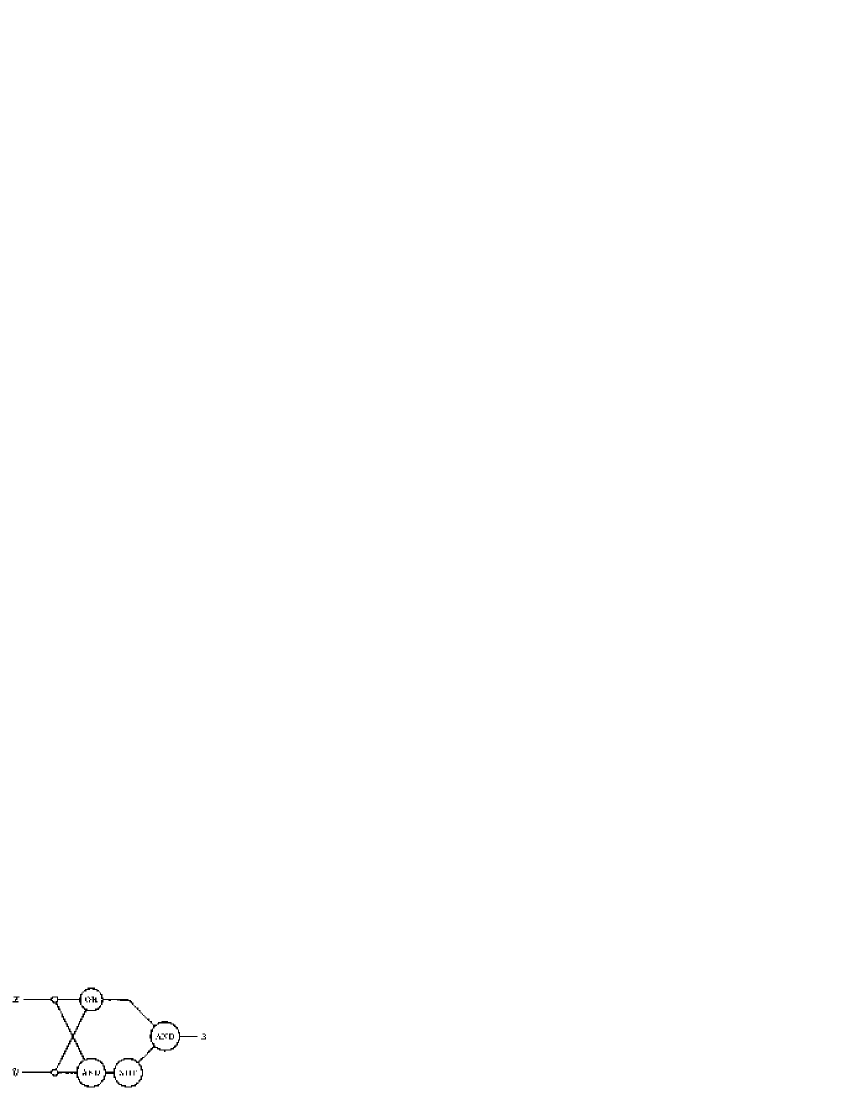
Figure 1: A circuit to compute the exclusive-or (xor) function, $z=x\;\text{{xor}}\;y$, using and, or and not gates. Note that this circuit uses three implicit gates, two clone gates, shown as small circles, where wires split into two (to copy the input) and one swap gate (where the wires cross over). These implicit gates are fairly easy to implement in traditional electronic computers, but can cause problems in other designs and so cannot simply be ignored. Some authors even consider the wires which interconnect gates as non-trivial gates in their own right.

Although several different theoretical models are useful for abstract descriptions of computers, one of the most convenient approaches for describing how to build small computers is the circuit model, in which bits interact through gates which implement Boolean logic operations. One traditional set of classical gates is the one bit not gate together with two different two bit gates, and and or. These three gates are said to form an adequate set, in that any desired logic operation can be performed by building an appropriate circuit (see figure 1 for an example) using some combination of these three gates.

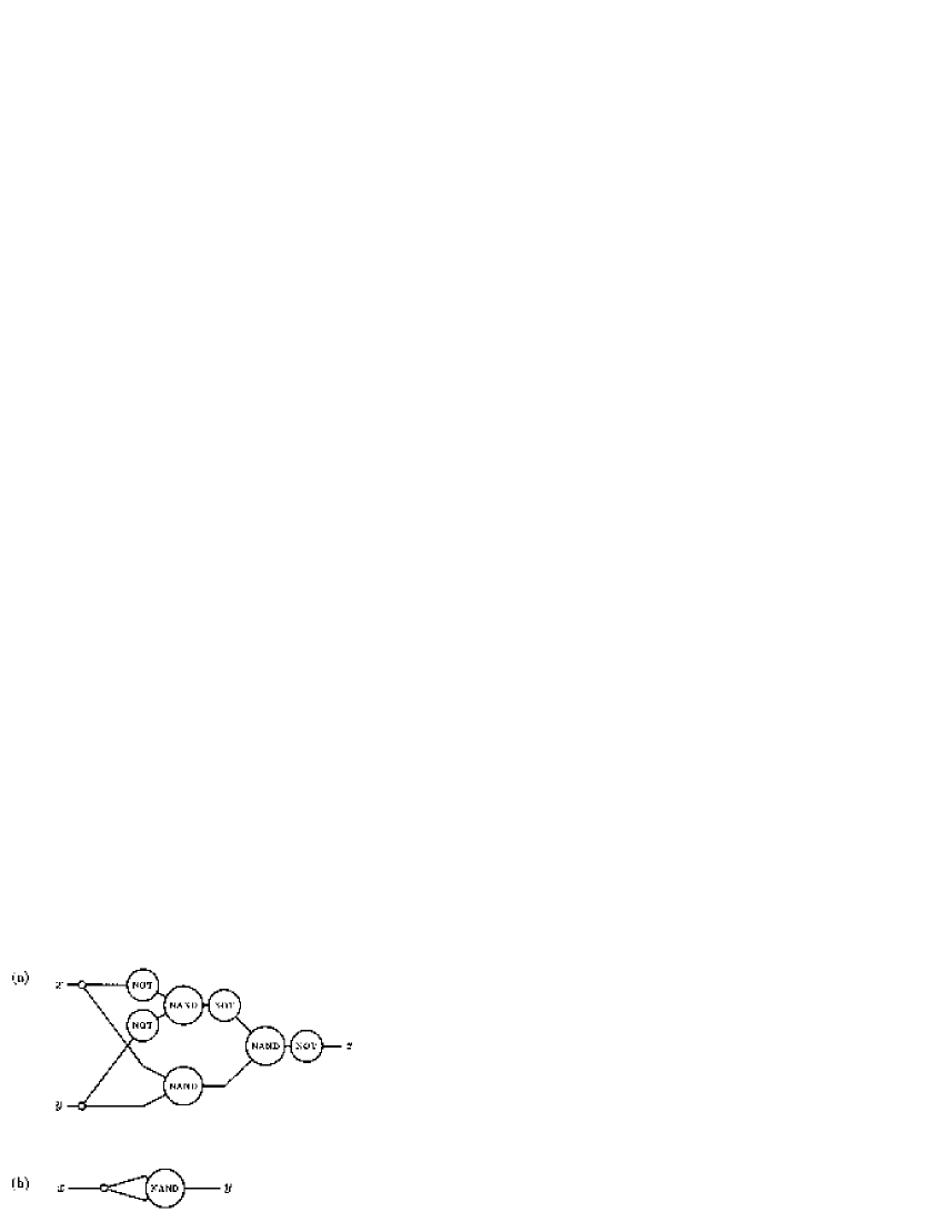
Figure 2: (a) A circuit to compute the exclusive-or (xor) function, $z=x\;\text{{xor}}\;y$, using only nand and not gates. This is not the best such circuit; simpler circuits are known, but this one preserves the basic structure seen in figure 1. (b) A circuit to implement a not gate, $y=\text{{not}}\;x$ using a nand gate. By combining circuits (a) and (b) it is possible to implement xor using only nand gates. Any other function may be computed in a similar fashion, and so nand is a universal gate. Note, however, that both circuits use implicit clone gates, while (a) also uses one implicit swap gate.

In fact it is not necessary to use all these gates: they can themselves all be obtained using combinations of nand gates (figure 2), and so the nand gate is universal for classical computation. It is, however, necessary to proceed with some caution, as several other “implicit” gates are also required, such as the clone gate, which makes a copy of a bit, and the swap gate, which allows two wires to cross one another.

This description works well with conventional computers, in which bit states are represented by voltages applied to wires, but it cannot be used with atomic computers. Atomic computers represent bit values using the quantum states of atomic systems, so a logic gate can neither create nor destroy bits; thus logic gates such as and, which have two input bits and only one output bit, are immediately ruled out. Similarly, atomic systems evolve under a series of unitary transformations, which correspond to reversible operations, while many of the operations described above are clearly not reversible. In order to build atomic computers, therefore, it is necessary to use a different approach, using only reversible logic operations.

III.2 Reversible computation

The theory of reversible computation Feynman:1996 ; Bennett:1973 ; Fredkin:1982 has been studied extensively and, perhaps surprisingly, it is simple to perform any logic operation in a reversible manner. The only irreversible operation required when performing a computation Landauer:1961 ; Landauer:1982 is the preparation of a well defined initial state, usually taken as having all bits in state 0; after this initialisation process the computation can be performed entirely reversibly.

The basic approach needed to achieve reversible logic can be summarised in two simple rules. First, any logical inputs to a gate must be preserved in the outputs; this is most simply achieved by copying them to output bits without change. Secondly, the output of the gate (here assumed for simplicity to comprise a single bit) must be combined in a reversible fashion with an additional auxiliary bit, for example by adding the two bits together using binary arithmetic modulo two.

Binary arithmetic modulo two, usually indicated by the symbol $\oplus$, has the useful properties that $x\oplus 0=0\oplus x=x$ and $x\oplus 1=1\oplus x=\mbox{\sc not}(x)$, while $x\oplus x=0$. A simple example of a reversible logic gate based on this approach is the controlled-not gate (see figure 3), which has two inputs, $x$ and $y$ and two corresponding outputs $x^{\prime}$ and $y^{\prime}$. The first input bit is copied to its output bit, so $x^{\prime}=x$, and is also combined with the second input bit to give $y^{\prime}=x\oplus y$. Thus a not gate is applied to the second bit (the target bit) if and only if the first bit (the control bit) is in state 1. Note that a controlled-not gate is completely reversible; indeed it can be reversed by simply applying the same gate again (that is, controlled-not is its own inverse). Furthermore, as $x\oplus y=x\;\text{{xor}}\;y$ the controlled-not gate is just a reversible xor gate.

Figure 3: The controlled-not gate, which plays a central role in reversible and quantum computation. The target bit is marked by a $\oplus$ symbol, indicating the close relationship with binary arithmetic modulo two; the control bit is marked by a dot and a vertical control line (the dot is important in drawings of larger circuits where a control line may have to cross lines representing other bits).

A more complex example is provided by the controlled-controlled-not gate, often called the Toffoli gate (figure 4), which plays a central role in reversible logic. This gate has three inputs, $x$, $y$ and $z$, and three corresponding outputs, $x^{\prime}$, $y^{\prime}$ and $z^{\prime}$. The first two input bits, which are the logical inputs, are copied unchanged, so that $x^{\prime}=x$ and $y^{\prime}=y$. A not gate is then applied to the third bit if and only if both $x$ and $y$ are in state 1; hence $z^{\prime}=z\oplus(\text{$x$ {\sc and} $y$})$. Thus this gate can be considered as a reversible equivalent to the conventional and and nand gates: to evaluate $x$ and $y$ just use a Toffoli gate with $z=0$, while for a nand gate set $z=1$.

Figure 4: The Toffoli gate, which gives $x^{\prime}=x$, $y^{\prime}=y$, and $z^{\prime}=z\oplus(\text{$x$ {\sc and} $y$})$.

The combination of the Toffoli gate with the controlled-not and simple not gates forms an adequate set, in that it is possible to build any other gate using only a combination of these gates (in particular controlled-not gates can also be used to build the two implicit gates, clone and swap, as shown in figure 5). Indeed, the Toffoli gate is universal in its own right, as a Toffoli gate can be easily converted into a controlled-not gate by setting $x=1$, and to a simple not gate by setting $x=y=1$.

(a)   (b) 

Figure 5: (a) The controlled-not gate can be used to reversibly clone a bit; (b) three controlled-not gates implement a swap gate.

III.3 Reversible function evaluation

Central to reversible computation is the idea of reversible function evaluation. I will initially assume that the function has a single bit as both input and output, but the generalisation to more complex functions is straightforward. This can be achieved by constructing a circuit with two inputs and two outputs, as shown in figure 6 (an $f$-controlled-not) and setting $b=0$. The two values of the function, $f(0)$ and $f(1)$, can then be evaluated by setting $a=0$ and $a=1$ respectively. The $f$-controlled-not gate can itself be built out of simpler gates, such as those described above; in most cases this will also require a number of ancilla bits to hold intermediate results. For simplicity these ancilla bits are usually omitted from diagrams such as figure 6.

Figure 6: The $f$-controlled-not gate, for reversible function evaluation: $a^{\prime}=a$ and $b^{\prime}=b\oplus f(a)$.

IV Quantum computation

We now have all the basic elements needed to describe how quantum computers could be used to extend our computational abilities. While large scale quantum algorithms, such as Shor’s algorithm, are too complex to describe here, the basic ideas are relatively simple.

As described above, a quantum mechanical two-level system can be used to build a reversible classical computer by using the two eigenstates of the system to represent bits in logical states 0 and 1. For example, the two Zeeman levels of a spin-$\frac{1}{2}$ nucleus in a magnetic field, $|\alpha\rangle$ and $|\beta\rangle$, would be suitable for this purpose. For simplicity the two states are usually denoted $|0\rangle$ and $|1\rangle$, allowing quantum computation to be described without reference to any particular implementation; this choice of basis set is called the computational basis. The system will not be confined to these two eigenstates, however, but can also be found in superpositions, such as

$$\frac{|0\rangle+|1\rangle}{\sqrt{2}}$$ (1)

(the $\sqrt{2}$ term is necessary to ensure that the state is normalised). For this reason a quantum mechanical two level system has much more freedom than a classical bit, and so is called a quantum bit, or qubit for short. A qubit in a superposition state is (in some sense) in both of the states contributing to the superposition at the same time, so a qubit can simultaneously occupy two different logical states.

Computational circuits are implemented within quantum computers by performing physical manipulations so that the computer evolves under a propagator which implements the desired unitary transformation. Just as circuits can be built up from gates these propagators can be assembled from simpler elements, and so these propagators are often referred to as circuits, even though their physical implementation may bear little resemblance to conventional electrical circuits. As before, this abstract model allows quantum computers to be described in a device-independent fashion.

As discussed below, it is possible to construct any quantum circuit by combining a small number of simple propagators, usually called gates. These gates only affect one or two qubits at a time, and so it is perfectly practical to describe their propagators explicitly, for example as a matrix. A matrix description clearly depends on the choice of basis set, but the usual choice is to work in the computational basis, in which the basis vectors correspond with the different logical states of the computer; thus for a two qubit gate the basis set is $\{|00\rangle,|01\rangle,|10\rangle,|11\rangle\}$. In many proposed physical implementations of quantum computers, such as NMR, this basis set is also the natural basis for the system, as the basis states are eigenstates of the background Hamiltonian.

IV.1 Quantum parallelism

The central feature underlying all quantum algorithms is the idea of quantum parallelism, which in turns stems from the ability of quantum systems to be found in superposition states. Consider once again the reversible circuit for function evaluation (figure 6). This can be achieved by constructing a propagator, $U_{f}$, applied to two qubits, which performs

$$|a\rangle|b\rangle\stackrel{{\scriptstyle U_{f}}}{{\longrightarrow}}|a\rangle|b\oplus f(a)\rangle$$ (2)

and setting $|b\rangle=|0\rangle$. The two values of the function, $f(0)$ and $f(1)$, can then be evaluated by setting $|a\rangle=|0\rangle$ and $|a\rangle=|1\rangle$ as before. Now consider the effect of applying this circuit when the first qubit is in a superposition described by equation 1 and the second qubit is in state $|0\rangle$ . This can be easily calculated as quantum mechanics is linear, and so the effect of applying a gate to a superposition is a superposition of the results of applying the gate to the two eigenstates. Hence the result is

$$\frac{\left(|0\rangle+|1\rangle\right)}{\sqrt{2}}|0\rangle\stackrel{{\scriptstyle U_{f}}}{{\longrightarrow}}\frac{|0\rangle|f(0)\rangle+|1\rangle|f(1)\rangle}{\sqrt{2}}.$$ (3)

Thus the quantum computer has simultaneously evaluated the values of $f(0)$ and $f(1)$.

When applied to more complex systems, quantum parallelism has potentially enormous power. Consider a function for which the input is described by $n$ bits, so that there are $2^{n}$ possible inputs (since $n$ bits can be used to describe any integer between 0 and $2^{n}-1$); a quantum computer using $n$ qubits as inputs can evaluate the function over all of these $2^{n}$ inputs in one step. In effect a quantum computer with $n$ input qubits appears to have the computational power of $2^{n}$ classical computers acting in parallel. Unfortunately it is not always possible to use this quantum parallelism in any useful way. Performing parallel function evaluation over $n$ qubits will result in a state of the form

$$\frac{\sum_{i=0}^{2^{n}-1}|i\rangle|f(i)\rangle}{2^{n/2}},$$ (4)

which is a superposition of the $2^{n}$ possible inputs, each entangled with its own function value. If any attempt is made to measure the state of the system, then the superposition will collapse into one of its component values, $|r\rangle$$|f(r)\rangle$, where the value of $r$ is chosen at random. Thus even though it seems possible to evaluate the function over its $2^{n}$ input values, it is only possible to obtain one of these values.

It is, however, sometimes possible to obtain useful information in a more subtle way. In some cases, the answer of interest does not depend on specific values, $f(r)$, but only on global properties of the function itself. This is the basis of both Deutsch’s toy algorithm and Shor’s quantum factoring algorithm.

IV.2 Deutsch’s algorithm

Deutsch’s algorithm Deutsch:1986 ; Deutsch:1992 ; Cleve:1998 was the first quantum algorithm to be discovered, and is one of the few quantum algorithms simple enough to describe here. The problem can be described in terms of function evaluation, but a more concrete picture can be obtained by thinking about coins. Normal coins have two different faces, conventionally called heads and tails, but fake coins can be obtained which have the same pattern on both faces.

Consider an unknown coin, which could be either a normal coin or a fake coin. In order to determine which type it is, it would seem necessary to look at both sides to find out whether they showed heads or tails, and then see whether these two results were the same (a false coin) or different (a true coin). With a quantum device, however, it would be possible to look at both sides simultaneously, and thus determine whether the coin was normal or fake in a single glance.

The trick lies in abandoning any attempt to determine the pattern shown on either side of the coin; instead one must simply ask whether the two faces are the same or different. This is a property not of the individual faces of the coin, but of the whole coin, and thus may be extracted from a state of the kind described by equation 3. A more detailed explanation of this approach is given in Section XI.

IV.3 Quantum gates

Just as classical reversible computations can be performed using circuits built up out of reversible gates, quantum circuits can be constructed using quantum gates DiVincenzo:1998b . Unlike classical circuits, however, quantum circuits can include gates which generate and analyse qubits which are in superpositions of states.

One such gate is the single qubit Hadamard gate, H, which implements the transformations

$$|0\rangle\stackrel{{\scriptstyle\textsc{H}}}{{\longrightarrow}}(|0\rangle+|1\rangle)/\sqrt{2}$$ (5)

$$|1\rangle\stackrel{{\scriptstyle\textsc{H}}}{{\longrightarrow}}(|0\rangle-|1\rangle)/\sqrt{2}$$ (6)

As discussed below, this is closely related to a $90^{\circ}$ pulse, but differs in some subtle ways; in particular the Hadamard is its own inverse.

The Hadamard gate is useful as it takes a qubit in an eigenstate to a uniform superposition of states. By analogy one can define multi-qubit Hadamard gates which take a quantum register into a uniform superposition of all its possible values:

$$|00\rangle\stackrel{{\scriptstyle\textsc{H}}}{{\longrightarrow}}(|00\rangle+|01\rangle+|10\rangle+|11\rangle)/2.$$ (7)

This can be easily achieved by applying a one qubit Hadamard to each qubit.

Another important property of the Hadamard gate can be seen by examining the right hand sides of equations 5 and 6. These differ only by the presence of a minus sign, so the two superpositions differ only by the phase with which the two eigenstates are combined. The ability of the Hadamard gate to convert such phase differences into different eigenstates plays a central role in many quantum algorithms.

IV.4 Universality of quantum gates

The gates we have seen so far are enough to explain some simple quantum algorithms; for example, Deutsch’s algorithm can be described using only Hadamard gates and reversible function evaluation gates. It is, however, useful to consider other more general quantum gates; indeed as any unitary transformation can be considered as a quantum gate, we may need to consider an infinite number of gates.

Within classical models of computation (both reversible and irreversible) it is possible to construct any desired gate by combining copies of a small number of simple gates. A similar situation applies in quantum computation, but in this case there are an infinite number of possible gates (even if we restrict ourselves to single qubit gates, any rotation around any axis constitutes a valid one qubit gate). Clearly it cannot be possible to construct an infinite number of different gates by combining a finite number of simpler gates, but it is possible to simulate any gate to any desired accuracy Deutsch:1989 ; Barenco:1995a , which is good enough. Perhaps surprisingly there exists a very large number of two qubit gates which are universal in this restricted sense, in that it is possible to simulate any desired gate (that is, any unitary transformation) using only one of these universal gates together with its twin, obtained by swapping the roles of the two qubits. Indeed, mathematically speaking, almost all two qubit gates are universal Barenco:1995c ; Deutsch:1995 ; Lloyd:1995 .

While mathematically interesting, this result is of little immediate practical implication for most possible implementations of a quantum computer, as it is usually more sensible to use a larger and more convenient set of gates. As one qubit gates are usually much simpler to perform than gates involving two or more qubits, it is often reasonable to assume that any one qubit gate (or, at least a reasonable approximation to it) is available. The combination of this set of one qubit gates with any single non-trivial two qubit gate, such as the controlled-not gate forms an adequate set Barenco:1995a , from which any other gate may be built with relative ease.

V Building NMR quantum computers

While it would in principle be possible to use a wide range of different approaches to build a quantum computer, all the main proposals to date Macchiavello:2000 ; Bouwmeester:2000 have used broadly similar approaches, based on the quantum circuit model outlined above. This model contains five major components, each of which must be implemented in order to construct a working computer DiVincenzo:2000 . Four central components can all be implemented within NMR systems as described below, while the fifth component, error correction, is discussed in Section XII.

V.1 Qubits

The first of these requirements, a set of qubits, appears easy to achieve, as the two spin states of spin-$\frac{1}{2}$ nuclei in a magnetic field provide a natural implementation. However, one important feature which distinguishes NMR quantum computers from other suggested implementations is that NMR studies not a single isolated quantum system, but rather a very large number (effectively an ensemble) of such systems. Thus an NMR quantum computer is actually an ensemble of indistinguishable computers, one on each molecule in the NMR sample. This has a number of subtle and important consequences as discussed below.

V.2 Logic gates

In order to perform an arbitrary computation it is necessary to implement arbitrary quantum logic circuits. This can be achieved as long as it is possible to implement an adequate set of gates, which can be combined together to implement any other desired gate. While many different sets of gates are possible, a simple approach is to implement the set of all possible one qubit gates, together with one or more non-trivial two qubit gates Barenco:1995a .

One qubit gates correspond to rotations of a spin within its own one-spin Hilbert space, which can be readily achieved using RF fields. Note that it is necessary to apply these rotations selectively to individual qubits. In most other suggested implementations of quantum computation Macchiavello:2000 ; Bouwmeester:2000 this is easily achieved using some type of spatial localisation: the physical objects implementing the qubits are located at well defined and distinct locations in space. This approach is not possible in NMR, as each qubit is implemented using an ensemble of nuclei, each of which is located at a different place in the NMR sample, and all of which are undergoing rapid motion. Instead different qubits are implemented using different nuclei in the same molecule, and they are distinguished using the different resonance frequencies of each nucleus.

Two qubit gates, such as the controlled-not gate, are more complicated as they involve conditional evolution (that is, the evolution of one spin must depend on the state of the other spin), and thus require some interaction between the two qubits. The J-coupling in NMR is well suited to this purpose. Note that all the different nuclei making up an NMR quantum computer must participate in a single coupling network. It is not necessary (or even desirable) that all the nuclei are directly coupled together, but they must be connected, directly or indirectly, by some chain of resolved couplings. Since J-coupling only occurs within a molecule, and does not connect different molecules, we can treat an ensemble of molecules as an ensemble of identical mutually isolated computers.

V.3 Initialisation

Quantum logic gates transform qubits from one state to another, but this is only useful if the qubits start off in some well defined initial state. In practice it is sufficient to have some method for reaching any one initial state, and the obvious choice is to have all the qubits in the $|0\rangle$ state, corresponding to a clear operation. Any other desired starting state can then be easily obtained.

When, as for NMR, the computational basis coincides with the natural basis of the quantum system it should in principle be easy to implement clear as it takes the quantum computer to its energetic ground state, and this can be achieved by some cooling process. Unfortunately this approach is not practical in NMR as the Zeeman energy gap is small compared with the Boltzman energy at any reasonable temperature; thus at room temperature the population of all the states will be almost equal, with only small deviations (around one part in $10^{4}$) from the average. Techniques for enhancing spin polarization Jones:2000d , such as optical pumping Walker:1997 ; Navon:1996 ; Pietrass:1999 , and the use of para-hydrogen Natterer:1997 ; Duckett:1999 ; Hubbler:2000 allow this deviation to be increased, but with the exception of optically pumped noble gases it has so far proved impossible to even approach a pure ground state system.

This apparent inability to implement the clear operation led to NMR being rejected as a practical technology for implementing quantum computers. Recently, however, it was realised Cory:1996 that this conclusion was over hasty, as with an ensemble quantum computer it is not actually necessary to produce a pure ground state; instead it suffices to produce a state which behaves in the same manner as the pure ground state. This point can be clarified by considering the density matrix describing a single isolated spin-half nucleus. This exhibits nearly equal populations for the two eigenstates, but with a slight excess in the (low energy) $|0\rangle$ state compared with the (slightly higher energy) $|1\rangle$ state. No NMR signal will be observed from the equal populations, as the signals from different molecules will cancel out, but a small signal can be seen which arises from the deviations away from the average. Thus, ignoring questions of signal intensity, for a single isolated nucleus the thermodynamic equilibrium state is indistinguishable from a pure $|0\rangle$ state.

States of this kind are often called pseudo-pure states, or effective pure states Cory:1996 ; Cory:1997 ; Gershenfeld:1997 . Unfortunately the simple approach outlined above does not work for larger spin systems, as the pattern of population deviations is more complicated, and does not have the desired form. Several different techniques have, however, been developed to tackle this problem.

V.4 Readout

The last stage in any quantum computation is to characterise the final state of the system, so that the result of the computation may be read out. Just as for initialisation, a range of different approaches have been used, but all these approaches combine two major elements. For simplicity I will assume that the computation ends with the result qubits in eigenstates; thus it is only necessary to determine whether a given qubit is in (the pseudo-pure) state $|0\rangle$ or $|1\rangle$.

The simplest approach is to apply a $90^{\circ}$ pulse to the corresponding spin, and observe the NMR spectrum Jones:1998a . Since $|0\rangle$ corresponds to the ground state, a qubit in $|0\rangle$ will give rise to an absorption line; correspondingly a qubit in state $|1\rangle$ will give an emissive signal. It is, of course, necessary to acquire some sort of reference signal, in order to distinguish between these two extremes, but this can be easily achieved by acquiring the spectrum of the pseudo-pure initial state.

The second major approach Chuang:1998a is to determine the state of one qubit by analysing the multiplet structure within the spectrum of a neighbouring spin. If several spins are coupled together, then individual lines within a multiplet can be assigned to specific states of these neighbours. Thus, the spectrum of one spin can give information on the states of several different qubits.

V.5 Some two spin systems

While a number of different systems have been used to build small NMR quantum computers, all their major features can be explored using two different two-qubit systems which were used in the earliest demonstrations of NMR quantum computation Jones:1998a ; Chuang:1998a . The most important difference between these systems is that one uses a homonuclear two-spin system, while the other is heteronuclear.

The first example system uses the two ${}^{1}\rm H$ nuclei of partially deuterated cytosine in $\rm D_{2}O$ (see figure 7). As this system is homonuclear it is possible to excite both nuclei with a single hard pulse, and to observe both nuclei in the same spectrum. Another more subtle advantage is that the pattern of Boltzmann populations is simpler in homonuclear systems than in their heteronuclear counterparts. There are, however, two significant disadvantages of such as system. Firstly the two ${}^{1}\rm H$ multiplets have relatively similar frequencies, as they lie only about $\rm 1.51\,ppm$ apart, and thus it is necessary to use soft frequency selective pulses Freeman:1997 (or sequences of hard pulses and delays with equivalent effects) in order to address the spins individually. Secondly, the J-coupling between the two spins is relatively small (about $\rm 7\,Hz$), and so controlled gates take a fairly long time to implement. It would, of course, be possible to choose a different molecule, in which the chemical shift difference or J-coupling was larger, but it is difficult to improve one without making the other worse. While it is unlikely that cytosine is the absolutely optimal choice, no other homonuclear ${}^{1}\rm H$ system would be very much better.

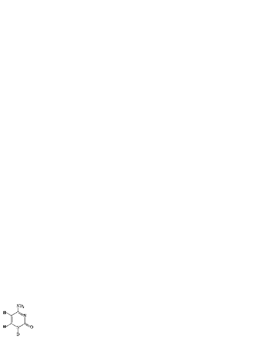
Figure 7: The structure of partially deuterated cytosine obtained by dissolving cytosine in $\rm D_{2}O$; the three protons bound to nitrogen nuclei exchange with solvent deuterons, leaving two ${}^{1}\rm H$ nuclei as an isolated two spin system (all other nuclei can be ignored).

The heteronuclear alternative is probably the most widely used two qubit NMR system. It is based on the ${}^{1}\rm H$ and ${}^{13}\rm C$ nuclei in ${}^{13}\rm C$-labeled chloroform. This has the huge advantage that it is possible to separately excite the two spins using hard pulses, rendering selective excitation essentially trivial. Furthermore, the relatively large size of the J-coupling allows two qubit gates to be performed much more rapidly than in homonuclear systems. In this heteronuclear system it is not possible to acquire signals from both spins simultaneously, but this is not a major problem as it is possible to determine the states of both spins by examining either the ${}^{1}\rm H$ or the ${}^{13}\rm C$ spectrum. Similarly, the complex pattern of populations over the four energy levels of this system does not fit with the original scheme for generating pseudo-pure states; however, some more modern schemes are in fact simpler to implement in heteronuclear systems.

Considering all these issues together, it is not easy to say whether it is better to use homonuclear or heteronuclear systems to implement two qubit NMR quantum computers: heteronuclear systems are perhaps simpler to work with, but homonuclear systems give more elegant results. With larger spin systems the issues become even more complex, and a wide range of options have been explored. It is clear, however, that the simplest approach of using a fully heteronuclear spin system is unlikely to be practical beyond five qubit systems, as there are only 5 “obvious” spin-half nuclei which can be used (${}^{1}\rm H$, ${}^{13}\rm C$, ${}^{15}\rm N$, ${}^{19}\rm F$ and ${}^{31}\rm P$). In practice NMR quantum computers with more than three qubits are likely to include two or more spins of the same nuclear species; it is, therefore, essential to consider how computation can be performed in homonuclear systems.

V.6 Scaling the system up

The requirements outlined above are adequate for building small quantum computers, suitable for simple demonstrations of quantum information processing. If, however, one wishes to build a large scale quantum computer, suitable for performing interesting computations, then it is necessary to consider whether the approaches used are limited to such small systems, or whether (and if so, how) they can be scaled up. A fifth requirement for practical quantum computation DiVincenzo:2000 , the implementation of fault-tolerant quantum error correction, is described in Section XII.

This is an important practical question, but not one which will be addressed in detail here. The problems of scaling up NMR quantum computers are formidable, and have been well described elsewhere Jones:2000d ; Warren:1997 ; Gershenfeld:1997b . Most authors now agree that NMR approaches are likely to be limited to computers containing 10–20 qubits; this is significantly smaller than estimates of the size required to perform useful computations (50–300 qubits). Furthermore the apparent inability of NMR systems to perform efficient quantum error correction rules out their use for many types of problem.

The fundamental difficulties involved in scaling up current NMR quantum computers to large sizes have led some authors to suggest that this approach does not actually implement real quantum computation at all. This is a quite subtle question which will be discussed further in Section XIII below.

VI Qubits and NMR spin states

Traditional designs for quantum computers comprise a number of two-level systems which interact with one another and have some specific interaction with the outside world, through which they can be monitored and controlled, but are otherwise isolated. NMR systems are rather different: a typical NMR sample comprises not one spin-system, but a very large number of copies, one from each molecule in the sample, effectively forming an ensemble of copies. Traditional quantum computers are usually described using Dirac’s bra(c)ket notation Goldman:1988 , but NMR systems are better described using density matrices, usually written in the product operator basis Sorensen:1983 , which has a number of important consequences. It is possible to draw close analogies between the states of traditional quantum computers and those used in descriptions of NMR systems Jones:1998d , but it is necessary to proceed with caution.

VI.1 One qubit states

A single qubit can be in either of its two eigenstates, $|0\rangle$ and $|1\rangle$, or in some linear superposition of them. Such a state is most conveniently written as a column vector in Hilbert space, for example

$$|\psi\rangle=\begin{pmatrix}c_{0}\\ c_{1}\end{pmatrix}.$$ (8)

NMR quantum computers cannot be properly described in this way; instead they must be described using the corresponding density matrix

$$\rho=|\psi\rangle\langle\psi|=\begin{pmatrix}c_{0}^{*}c_{0}&c_{1}^{*}c_{0}\\ c_{0}^{*}c_{1}&c_{1}^{*}c_{1}\end{pmatrix}$$ (9)

which can then be decomposed as a sum of the four Pauli basis states or their product operator equivalents, $\mbox{$\frac{1}{2}$}E$, $I_{x}$, $I_{y}$, and $I_{z}$.

Consider first the eigenstates, $|0\rangle$ and $|1\rangle$, which correspond to the density matrices

$$|0\rangle\langle 0|=\begin{pmatrix}1&0\\ 0&0\end{pmatrix}=\mbox{$\frac{1}{2}$}E+I_{z}$$ (10)

and

$$|1\rangle\langle 1|=\begin{pmatrix}0&0\\ 0&1\end{pmatrix}=\mbox{$\frac{1}{2}$}E-I_{z}$$ (11)

respectively. As all NMR observables are traceless, multiples of the unit matrix can be added to density matrices at will, and so as far as any NMR experiment is concerned the density matrix $I_{z}$ is equivalent to $|0\rangle$, while $-I_{z}$ is equivalent to $|1\rangle$. In the language introduced above, $I_{z}$ and $-I_{z}$ are pseudo-pure states, corresponding to $|0\rangle$ and $|1\rangle$ respectively. This approach cannot, however, be extended to larger spin systems without modifications.

Next consider superpositions, such as $(|0\rangle+|1\rangle)/\sqrt{2}$, with its corresponding density matrix

$$\begin{pmatrix}\mbox{$\frac{1}{2}$}&\mbox{$\frac{1}{2}$}\\ \mbox{$\frac{1}{2}$}&\mbox{$\frac{1}{2}$}\end{pmatrix}=\mbox{$\frac{1}{2}$}E+I_{x}.$$ (12)

As before multiples of the unit matrix can be ignored, and so $(|0\rangle+|1\rangle)/\sqrt{2}$ is equivalent to $I_{x}$. Similarly $|0\rangle+i|1\rangle$ is equivalent to $I_{y}$, while $|0\rangle-|1\rangle$ is equivalent to $-I_{x}$. Just as single qubit eigenstates are closely related to one spin magnetizations, their superpositions are closely related to one spin coherences.

VI.2 Two qubit states

While there is a simple relationship between qubit states and NMR states for a single qubit (a one spin system), this relationship is more complicated in systems with two or more qubits Jones:1998d . Typically quantum algorithms start with all qubits in state $|0\rangle$, which for a two-qubit computer is the state $|00\rangle$. The corresponding density matrix

$$|00\rangle\langle 00|=\begin{pmatrix}1&0&0&0\\ 0&0&0&0\\ 0&0&0&0\\ 0&0&0&0\end{pmatrix}$$ (13)

is not the same as the thermal equilibrium density matrix

$$I_{z}+S_{z}=\begin{pmatrix}1&0&0&0\\ 0&0&0&0\\ 0&0&0&0\\ 0&0&0&-1\end{pmatrix}.$$ (14)

The ideal density matrix (Eq. 13) can, however, be decomposed as the sum of four product operators:

$$|00\rangle\langle 00|=\mbox{$\frac{1}{2}$}\left(\mbox{$\frac{1}{2}$}E+I_{z}+S_{z}+2I_{z}S_{z}\right),$$ (15)

and this sum (ignoring multiples of the unit matrix as usual) can be assembled using conventional NMR techniques, as described below.

Superpositions can be treated in much the same way, but they are not directly related to NMR coherences in any very simple way. For example consider the state $(|00\rangle+|01\rangle)/\sqrt{2}$, in which the first spin is in state $|0\rangle$, while the second spin is in a superposition of states. The corresponding density matrix can be decomposed directly:

$$\begin{pmatrix}\mbox{$\frac{1}{2}$}&\mbox{$\frac{1}{2}$}&0&0\\ \mbox{$\frac{1}{2}$}&\mbox{$\frac{1}{2}$}&0&0\\ 0&0&0&0\\ 0&0&0&0\end{pmatrix}=\mbox{$\frac{1}{2}$}\left(\mbox{$\frac{1}{2}$}E+I_{z}+S_{x}+2I_{z}S_{x}\right),$$ (16)

but there is a more subtle approach. Note that $(|00\rangle+|01\rangle)/\sqrt{2}$ can be written as a product of single qubit states

$$\frac{|00\rangle+|01\rangle}{\sqrt{2}}=\frac{|0\rangle(|0\rangle+|1\rangle)}{\sqrt{2}},$$ (17)

and so the corresponding density matrix can also be decomposed as a direct product of equations 10 and 12:

$$\begin{split}\begin{pmatrix}1&0\\ 0&0\end{pmatrix}\otimes\begin{pmatrix}\raisebox{1.72218pt}{$\scriptstyle\frac{1}{2}$}&\raisebox{1.72218pt}{$\scriptstyle\frac{1}{2}$}\\ \raisebox{1.72218pt}{$\scriptstyle\frac{1}{2}$}&\raisebox{1.72218pt}{$\scriptstyle\frac{1}{2}$}\end{pmatrix}&=\left(\mbox{$\frac{1}{2}$}E+I_{z}\right)\times\left(\mbox{$\frac{1}{2}$}E+S_{x}\right)\\ &=\mbox{$\frac{1}{2}$}\left(\mbox{$\frac{1}{2}$}E+I_{z}+S_{x}+2I_{z}S_{x}\right).\end{split}$$ (18)

Unlike the single qubit case, a simple superposition does not correspond directly to an NMR coherence, but instead to a complex mixture of coherences and populations. It is, however, rarely necessary to worry about this, as such states can be easily obtained from states like Eq. 13.

Finally consider superpositions of the form $(|00\rangle+|11\rangle)/\sqrt{2}$, which cannot be broken down into a product of one qubit states (such states are said to be entangled). As they cannot be factored it is necessary to decompose the corresponding density matrices directly. In this case

$$\begin{pmatrix}\mbox{$\frac{1}{2}$}&0&0&\mbox{$\frac{1}{2}$}\\ 0&0&0&0\\ 0&0&0&0\\ \mbox{$\frac{1}{2}$}&0&0&\mbox{$\frac{1}{2}$}\end{pmatrix}=\mbox{$\frac{1}{2}$}\left(\mbox{$\frac{1}{2}$}E+2I_{z}S_{z}+2I_{x}S_{x}-2I_{y}S_{y}\right),$$ (19)

which is a mixture of longitudinal two-spin order and $DQ_{x}$ double quantum coherence.

VII NMR logic gates

After the rather abstract discussions above, we now turn to the details of methods by which quantum logic gates can be (and have been) implemented within NMR.

VII.1 One qubit gates

Many one qubit logic gates can be implemented directly. For example, a simple not gate, which interconverts $|0\rangle$ and $|1\rangle$, can be implemented as a $180^{\circ}_{x}$ rotation Jones:1998d . Rotations about axes in the $xy$-plane can be achieved using RF pulses, while rotations about the $z$-axis can be accomplished either by using periods of free precession under the Zeeman Hamiltonian, or by composite $z$-pulses Freeman:1981 . This does not, however, cover the full range of gates which may be desired, as some of these correspond to rotations about tilted axes.

An obvious (and important) example is the Hadamard gate. While this superficially resembles a $90^{\circ}$ pulse, this resemblance is misleading, as the Hadamard gate is its own inverse. Clearly the Hadamard must correspond to a $180^{\circ}$ rotation, and a little thought reveals that this rotation occurs around an axis tilted at $45^{\circ}$ within the $xz$-plane. This could be achieved directly by using off-resonance excitation, but this has a number of practical difficulties. Alternatively it can be implemented using a composite pulse sequence, such as $45^{\circ}_{y}$–$180^{\circ}_{x}$–$45^{\circ}_{-y}$; as $180^{\circ}_{x}$–$45^{\circ}_{\pm y}$ can be replaced by $45^{\circ}_{\mp y}$–$180^{\circ}_{x}$ this three pulse sequence may be simplified to the two pulse sequence $90^{\circ}_{y}$–$180^{\circ}_{x}$ or $180^{\circ}_{x}$–$90^{\circ}_{-y}$.

In fact, when implementing quantum algorithms on NMR quantum computers it is rarely necessary or desirable to use a Hadamard gate, as it can generally be replaced by the NMR pseudo-Hadamard gate, a $90^{\circ}_{y}$ pulse Jones:1998d . As this gate is not self-inverse it is usually necessary to replace pairs of Hadamard gates by one pseudo-Hadamard and one inverse pseudo Hadamard ($90^{\circ}_{-y}$) gate. This is a simple example of a general rule in experimental implementations of quantum computation: rather than directly implementing the gates commonly used in theoretical descriptions, it is better to use simpler gates which are broadly functionally equivalent to them.

VII.2 Controlled-NOT gates

This approach is also applicable to the implementation of controlled two-qubit gates. While it is perfectly possible to implement a controlled-not gate, this is not necessarily the most sensible approach. The controlled-not gate can itself be assembled from simpler basic gates, and it may be more sensible to use these basic gates directly.

A natural way to implement a controlled-not gate is to use a three gate circuit, as shown in figure 8(a). The two boxes marked H are one qubit Hadamard gates, and the central gate (two circles connected by a control line) is a two qubit controlled $\pi$ phase-shift gate. This gate performs the transformation

$$|1\rangle|1\rangle\overset{\bm{\pi}}{\longrightarrow}-|1\rangle|1\rangle$$ (20)

while leaving all other states unchanged, and so is described by the matrix

$$\bm{\pi}=\begin{pmatrix}1&0&0&0\\ 0&1&0&0\\ 0&0&1&0\\ 0&0&0&-1\end{pmatrix}.$$ (21)

Unlike the controlled-not gate this phase shift gate is symmetric; it is not meaningful to ask which qubit the phase shift was applied to. Note that the other controlled-not gate, in which the roles of control and target qubit are reversed, can be constructed by simply moving the two Hadamard gates to the upper line.

(a)   (b) 

Figure 8: (a) A circuit for implementing a controlled-not gate; the two outer gates are one qubit Hadamard gates, while the central gate is a controlled $\pi$-phase-shift gate (see text for details). (b) A circuit for implementing a controlled-not gate on an NMR quantum computer; the one qubit Hadamard gates are replaced by pseudo-Hadamard (h) and inverse pseudo-Hadamard ($\text{h}^{-1}$) gates.

When implementing this circuit on an NMR quantum computer it is preferable to avoid using Hadamard gates, as these are difficult to implement. Instead these two gates are replaced by an inverse pseudo-Hadamard (a $90_{-y}$ pulse) and a pseudo-Hadamard gate (a $90_{y}$ pulse) respectively, as shown in figure 8(b).

To see how to implement the controlled phase shift gate it is best to break down the propagator, equation 21, using the product operator basis set. As this propagator is diagonal, it must arise from evolution under the diagonal operators $I_{z}$, $S_{z}$, $2I_{z}S_{z}$ and (for completeness) $\raisebox{1.72218pt}{$\scriptstyle\frac{1}{2}$}E$. It can be decomposed in two ways,

$$\bm{\pi}=\exp\left[-i\times\pi/2\left(\raisebox{1.72218pt}{$\scriptstyle\frac{1}{2}$}E-I_{z}-S_{z}+2I_{z}S_{z}\right)\right],$$ (22)

or

$$\bm{\pi}=\exp\left[-i\times\pi/2\left(-\raisebox{1.72218pt}{$\scriptstyle\frac{1}{2}$}E+I_{z}+S_{z}-2I_{z}S_{z}\right)\right].$$ (23)

The choice between these two decompositions is simply a matter of experimental convenience.

The use of $\raisebox{1.72218pt}{$\scriptstyle\frac{1}{2}$}E$ in these equations might appear to give rise to difficulties, as this is not normally considered as a product operator which can arise in NMR Hamiltonians. In fact it is of no significance at all, as the effect of the $\raisebox{1.72218pt}{$\scriptstyle\frac{1}{2}$}E$ term is simply to impose a global phase shift. Such global phase shifts have no physical meaning, and cannot be detected; note that these global phase shifts have no effect on density matrix (or product operator) descriptions of the spin system. Physically this corresponds to the fact that there is no absolute zero against which energies may be measured.

Implementing these propagators (equations 22 and 23) is fairly straightforward. The pure spin–spin coupling term ($2I_{z}S_{z}$) can be generated using conventional spin-echo techniques, while the two Zeeman Hamiltonians ($I_{z}$ and $S_{z}$) can be achieved by appropriately timed periods of free precession, by the use of composite $z$-pulses, or most simply by just rotating the RF reference frame. As the three terms all commute, they need not be applied simultaneously, but can be applied in any order. When the individual elements making up the propagator are combined, it is frequently possible to combine or cancel individual pulses, thus simplifying the whole sequence. This results in a wide variety of possible pulse sequences, and the choice among them is largely a matter of taste. For example, one possible sequence for implementing $\bm{\pi}$ is

$$\frac{1}{4J}-180_{x}-\frac{1}{4J}-90_{x}-90_{-y}-90_{x}$$ (24)

where all pulses are applied to both spins.

While the possible pulse sequences differ in detail they have one feature in common: an evolution time of $1/2J$ (occasionally $3/2J$) during which the spins evolve under the spin–spin coupling, so that the antiphase condition is achieved. This is, of course, the central feature of coherence transfer sequences, such as INEPT, indicating the close relationship between controlled two qubit gates and coherence transfer.

VII.3 Other two qubit gates

While the controlled-not gate is important it is not the only two-qubit gate worth considering: while it is possible to construct any desired gate using only controlled-not gates and one-qubit gates, it is usually more efficient to use a wider repertoire of basic gates.

One simple and important example is the controlled square-root of not gate, which plays a central role in traditional constructions of the three-qubit Toffoli gate DiVincenzo:1998b ; this is one member of a more general family of $n^{\text{th}}$ roots of not. Such gates can be built in much the same way as controlled-not gates, except that the controlled $\pi$ phase-shift gate must be replaced by the more general transformation

$$|1\rangle|1\rangle\overset{\bm{\phi}}{\longrightarrow}e^{i\phi}|1\rangle|1\rangle$$ (25)

with $\phi=\pi/n$. Clearly $\bm{\phi}$ can be constructed in much the same way as $\bm{\pi}$, equation 23.

VII.4 Gates in larger spin systems

The approaches described above can be easily implemented in two spin systems, allowing quantum computers with two qubits to be easily constructed. With larger spin systems, however, the process can become much more complicated Jones:2000d . It is not possible simply to use pulse sequences designed for two spin systems, as it is necessary to consider the evolution of all the additional spins in the system. In particular it may be necessary to refocus the evolution of these spins under their chemical shift and J-coupling interactions. The simplest method is to nest spin echoes within one another, so that all the undesirable interactions are removed, but this naïve approach requires an exponentially large number of refocusing pulses (that is, the complexity of the pulse sequence doubles with every additional spin). This problem can be overcome by using efficient refocusing sequences Jones:1999b ; Leung:1999b , which allow refocusing to be achieved with quadratic overhead.

It is, of course, rare to find a large spin system where all the couplings have significant size; in most cases long range couplings will be small enough to be neglected. This greatly simplifies the problem, both by reducing the number of couplings which have to be refocused, and by simplifying the echo sequences required Jones:1999b ; Linden:1999c . It might seem that it would be difficult to implement some logic gates in such a partially coupled spin system, as the necessary spin–spin couplings are missing. In fact this is not a problem, as long as every pair of spins is connected by some chain of couplings: quantum swap gates Madi:1998 ; Linden:1999b can be used to move quantum information along this chain.

VII.5 Multi qubit logic gates

Multi qubit logic gates are gates, such as the Toffoli gate, which perform controlled operations involving more than two qubits. Such gates can of course be implemented by constructing appropriate networks of one qubit and two-qubit gates DiVincenzo:1998b , but as the NMR Hamiltonian can contain terms connecting multiple pairs of spins it should be possible to build some such gates directly, with a significant saving in pulse sequence complexity. This is indeed the case, and several interesting results have been obtained Price:1999b ; Price:2000a .

VII.6 Single transition selective pulses

An alternative approach for building controlled two qubit gates is to use ultra-soft selective pulses Freeman:1997 , with excitation profiles so narrow that they pick out, for example, a single transition from within a doublet. This corresponds to only exciting the nucleus of interest when the neighbouring nucleus is in a certain state Barenco:1995b ; if the excitation corresponds to a $180^{\circ}$ pulse then this provides a simple way of constructing a controlled-not gate Linden:1998a . The relationship between this approach and the (more common) multiple pulse sequence approach is analogous to that between the old fashioned selective population transfer experiment Pachler:1973 and its more modern counterpart, INEPT Morris:1979 .

One advantage of this approach Linden:1998a ; Dorai:2000 is that it is relatively easy to extend it to multi qubit gates such as the Toffoli gate. This can be achieved by using a selective pulse which affects one of the four transitions of a spin coupled to two neighbours. A corresponding disadvantage is that in this case constructing a simple controlled-not gate requires either a selective pulse which excites two of the four transitions in such a system or the application of two single transition selective pulses in sequence.

The traditional Toffoli gate corresponds to inverting a qubit when two other qubits are in the state $|1\rangle$, but there is an entire family of related gates which effect an inversion for some given pattern of states. Each such gate corresponds to exciting a different transition in the multiplet, and so the entire family of gates can be achieved directly. In practice, however, the central regions of a multiplet can become quite crowded, with many lines nearly overlapping, and it will be difficult to select a single transition. By contrast the two transitions at the extreme ends of the multiplet will always be relatively well separated from their nearest neighbours, and it is best to concentrate on these two frequencies. Other gates can then be constructed by surrounding these basic gates with not gates applied to the neighbouring spins, thus permuting the identities of the lines in the multiplet.

VII.7 Geometric phase-shift gates

A third approach for implementing NMR quantum computation, based on the use of geometric phase-shift gates, has recently been described Jones:2000a ; Ekert:2000a . Like the conventional approach it relies on controlled phase-shift gates, but the phase shifts are generated using geometric phases Shapere:1989 , such as Berry’s phase Berry:1984 , rather than the more conventional dynamic phases. Berry phases have been demonstrated in a wide variety of systems Shapere:1989 , including NMR Suter:1987 ; Goldman:1996 and the closely related technique of NQR Tycko:1987 ; Appelt:1994 ; Jones:1997 , and can be used to implement controlled phase shift gates in NMR systems Jones:2000a ; Ekert:2000a . This approach has few advantages for NMR quantum computation, but may prove useful in other systems Ekert:2000a .

VIII Initialisation and NMR

As it is impractical to cool down NMR spin systems to their ground state Jones:2000d ; Warren:1997 ; Gershenfeld:1997b , initialisation of an NMR quantum computer in practice means assembling an appropriate pseudo-pure state. This approach is useful only if some practical procedure for assembling such states can be devised.

For the simplest possible system (a single nucleus) the process is trivial, as the thermal equilibrium density matrix has the desired form, but with larger systems the situation is more complicated. The essential feature of a pseudo-pure state is that it has a diagonal density matrix in which the populations of all the spin states (the elements along the diagonal) are the same, with the exception of one state (normally $|\mathbf{0}\rangle=|000\dots 0\rangle$) which has a larger population. By contrast, at thermal equilibrium the spin state populations are distributed in accordance with the Boltzmann equation, and so exhibit a more complex variation. For a homonuclear two spin system the equilibrium density matrix (neglecting multiples of the identity matrix and an initial scaling factor) is $I_{z}+S_{z}$, while the desired pseudo-pure state is proportional to $I_{z}+S_{z}+2I_{z}S_{z}$ (equation 15).

The original approach for assembling pseudo-pure states, developed by Cory et al. Cory:1996 ; Cory:1997 , uses conventional NMR techniques. Assembling such a mixture using pulse sequences and field gradients is a fairly straightforward, if somewhat unusual, NMR problem. This process is commonly called spatial averaging, presumably a reference to the use of field gradients.

A second early approach, suggested by Gershenfeld and Chuang Gershenfeld:1997 , is to use a subset of the energy levels in a more complex spin system. For example, in a homonuclear three spin system it is possible to find a set of four energy levels which exhibit the pattern of populations corresponding to the pseudo-pure state of a two spin system. This approach, often called logical labeling, is elegant in principle but complex to apply in practice, and has only rarely been experimentally demonstrated.

More recently a variety of different approaches have been used, although these all combine elements of the two basic approaches above. The most popular technique, usually called temporal averaging Knill:1998 , works by performing many different experiments, each with a different initial state. For example, in a two qubit system, one might perform experiments starting from $I_{z}$, $S_{z}$, and $2I_{z}S_{z}$. If the spectra from these three experiments are then added together, the result is equivalent to a single experiment starting from a mixture of these states. Clearly temporal averaging and spatial averaging are related in much the same way as coherence selection methods based on phase cycling and gradients. Finally, a new approach combines these methods in a cunning way, using the analogy between multiple quantum coherence and so-called “cat” states to generate pseudo-pure states in a fairly efficient manner Knill:2000 .

VIII.1 Spatial averaging

The direct “spatial averaging” technique may be exemplified by the original sequence of Cory et al. Cory:1996 ; Cory:1997 for constructing a pseudo-pure state in a two spin system:

$$\begin{split}&I_{z}+S_{z}\\ \xrightarrow{\makebox[25.00003pt]{$\scriptstyle 60^{\circ}S_{x}$}}&I_{z}+{\raisebox{1.72218pt}{$\scriptstyle\frac{1}{2}$}}S_{z}-\raisebox{1.72218pt}{$\scriptstyle{\frac{\sqrt{3}}{2}}$}S_{y}\\ \xrightarrow{\makebox[25.00003pt]{$\scriptstyle\text{crush}$}}&I_{z}+{\raisebox{1.72218pt}{$\scriptstyle\frac{1}{2}$}}S_{z}\\ \xrightarrow{\makebox[25.00003pt]{$\scriptstyle 45^{\circ}I_{x}$}}&\raisebox{1.72218pt}{$\scriptstyle{\frac{1}{\sqrt{2}}}$}I_{z}-\raisebox{1.72218pt}{$\scriptstyle{\frac{1}{\sqrt{2}}}$}I_{y}+{\raisebox{1.72218pt}{$\scriptstyle\frac{1}{2}$}}S_{z}\\ \xrightarrow{\makebox[25.00003pt]{$\scriptstyle\text{couple}$}}&\raisebox{1.72218pt}{$\scriptstyle{\frac{1}{\sqrt{2}}}$}I_{z}+\raisebox{1.72218pt}{$\scriptstyle{\frac{1}{\sqrt{2}}}$}2I_{x}S_{z}+{\raisebox{1.72218pt}{$\scriptstyle\frac{1}{2}$}}S_{z}\\ \xrightarrow{\makebox[25.00003pt]{$\scriptstyle 45^{\circ}I_{-y}$}}&{\raisebox{1.72218pt}{$\scriptstyle\frac{1}{2}$}}I_{z}-{\raisebox{1.72218pt}{$\scriptstyle\frac{1}{2}$}}I_{x}+{\raisebox{1.72218pt}{$\scriptstyle\frac{1}{2}$}}2I_{x}S_{z}+{\raisebox{1.72218pt}{$\scriptstyle\frac{1}{2}$}}S_{z}+{\raisebox{1.72218pt}{$\scriptstyle\frac{1}{2}$}}2I_{z}S_{z}\\ \xrightarrow{\makebox[25.00003pt]{$\scriptstyle\text{crush}$}}&{\raisebox{1.72218pt}{$\scriptstyle\frac{1}{2}$}}I_{z}+{\raisebox{1.72218pt}{$\scriptstyle\frac{1}{2}$}}S_{z}+{\raisebox{1.72218pt}{$\scriptstyle\frac{1}{2}$}}2I_{z}S_{z}\\ \end{split}$$ (26)

where the sequence is described in product operator notation, “crush” indicates the application of a crush field gradient pulse, and “couple” indicates evolution under the scalar coupling for a time $1/2J$. Note that the two crush pulses must be applied along different axes, or with different strengths, to prevent undesired terms from being refocused.

Several alternative sequences for creating two spin pseudo-pure states have been developed; for example Pravia:1999

$$\begin{split}I_{z}+S_{z}&\xrightarrow{45^{\circ}(I_{x}+S_{x})}\xrightarrow{\text{couple}}\xrightarrow{30^{\circ}(I_{-y}+S_{-y})}\\ &\xrightarrow{\text{crush}}\sqrt{\frac{3}{8}}\left(I_{z}+S_{z}+2I_{z}S_{z}\right)\end{split}$$ (27)

where zero quantum terms (which in a homonuclear spin system will survive the crush pulse) have been neglected. This scheme works well in heteronuclear spin systems, but in homonuclear systems it is necessary to use a more complex approach to deal with the zero quantum terms.

These sequences can be generalised to larger spin systems, but this process is quite complex. For this reason most work on larger spin systems has used temporal averaging techniques. Recently, however, Knill et al. Knill:2000 have developed a general scheme based on cat states, which allows pulse sequences for any spin system to be developed. This approach is described below.

VIII.2 Logical labeling

Logical labeling Gershenfeld:1997 is most easily understood by examining the thermal equilibrium density matrix for a homonuclear three spin system:

$$I_{z}+S_{z}+R_{z}=\mbox{$\frac{1}{2}$}\left\{3,1,1,-1,1,-1,-1,-3\right\},$$ (28)

where the braces indicate a diagonal matrix defined by listing its diagonal elements. While this matrix does not have the right form for a three spin pseudo-pure state it is possible to select out four levels (corresponding to the states $|000\rangle$, $|011\rangle$, $|101\rangle$ and $|110\rangle$) which have the same population pattern as

$$I_{z}+S_{z}+2I_{z}S_{z}=\mbox{$\frac{1}{2}$}\left\{3,-1,-1,-1\right\},$$ (29)

and so this subset of levels can be used as a two spin pseudo-pure state.

It would be possible to use these states directly, but this would greatly complicate subsequent logic operations as there is no simple correspondence between these four states of the three spin system and the four basic states of a two spin system. Instead it is better to permute the populations of the various states, performing $|001\rangle\leftrightarrow|101\rangle$ and $|010\rangle\leftrightarrow|110\rangle$; these permutations can be achieved using controlled-not gates. At the end of this process the populations are given by

$$\mbox{$\frac{1}{2}$}\left\{3,-1,-1,-1,1,1,1,-3\right\},$$ (30)

so that the states $|000\rangle$, $|001\rangle$, $|010\rangle$ and $|011\rangle$ are in a pseudo-pure state. Note that these four states all have the first spin in state $|0\rangle$, and so the first spin acts as an ancilla spin, labeling the “correct” subspace.

Similar, but more complex, procedures can be used with larger spin systems Gershenfeld:1997 . The overhead required is fairly small; that is the number of pseudo-pure spins which can be encoded in a spin system is only slightly smaller than the size of the system. However, while these results are elegant the complexity of implementing logical labeling means that experimental demonstrations have so far been confined to three spin systems Dorai:2000 ; Vandersypen:1999 .

VIII.3 Temporal averaging

As discussed previously, temporal averaging Knill:1998 bears much the same relationship to spatial averaging as phase cycling does to the use of gradients to select coherence transfer pathways. The name can, however, be used to cover a variety of different approaches.

As described above (equation 15), a pseudo-pure state of a two spin system can be assembled as a mixture of three terms: $I_{z}$, $S_{z}$ and $2I_{z}S_{z}$. The simplest approach to temporal averaging is just to perform a computation starting from each of these states, and add the results together at the end. This is easily generalised to larger spin systems: for a system of $n$ spins it is necessary to perform $2^{n}-1$ separate experiments. In some simple experiments it is possible to show that only some of these starting states will give an observable signal Marx:2000 , and so it is unnecessary to perform experiments starting in other states. This permits substantial experimental simplifications, but it is not a general technique.

A better approach is to use the original scheme of Knill et al. Knill:1998 . The thermal equilibrium density matrix for a two spin system

$$I_{z}+S_{z}=\left\{1,0,0,-1\right\}$$ (31)

(where the braces have the same meaning as before) can be easily converted into two other states,

$$I_{z}+2I_{z}S_{z}=\left\{1,0,-1,0\right\}$$ (32)

and

$$S_{z}+2I_{z}S_{z}=\left\{1,-1,0,0\right\}.$$ (33)

These three states are related by simple permutations of the populations of the levels, which can be achieved using controlled-not gates. Adding together the three starting states gives

$$2\left(I_{z}+S_{z}+2I_{z}S_{z}\right)=\left\{3,-1,-1,-1\right\},$$ (34)

which is a pseudo-pure state. Adding together the spectra from computations started in these three states therefore gives the spectrum which would be produced from a pseudo-pure state.

Once again this process is easily generalised to larger spin systems. The most obvious approach is to average over the $2^{n}-1$ cyclic permutations of the populations in an $n$ spin system. This exhaustive averaging scheme is just as inefficient as the naïve approach outlined above, but Knill et al. Knill:1998 have shown that similar results can be achieved by averaging over much smaller numbers of states.

VIII.4 The use of “cat” states

The schemes described above are perfectly practical for small spin systems but are harder to use with larger systems. Recently Knill et al. Knill:2000 have described a simple approach which works for spin systems of any size and which can be used with either the gradient (spatial averaging) or phase cycling (temporal averaging) approaches. Their method is based on the properties of “cat” states, named by analogy with Schrödinger’s Cat. An $n$ qubit cat state is a superposition state of the form

$$\phi_{n}^{\pm}=\left(|00\dots 0\rangle\pm|11\dots 1\rangle\right)/\sqrt{2},$$ (35)

so that either all the $n$ qubits are in state $|0\rangle$, or all the qubits are in state $|1\rangle$. (In fact the relative phase of the two states contributing to the superposition can take any value between $0$ and $2\pi$, but it is convenient to restrict ourselves to the two values $0$ and $\pi$, giving rise to the factor of $\pm 1$.) States of this form are said to be entangled, and play a central role in quantum information processing and experimental tests of quantum mechanics. The role of entanglement in NMR quantum computers will be explored in more detail below, but for the moment it is sufficient to note that cat states are closely related to (but not simply equivalent to) multiple quantum coherence Jones:1998d .

As discussed above (equation 19) the two qubit cat state $\phi_{2}^{+}=(|00\rangle+|11\rangle)/\sqrt{2}$ (commonly called a Bell state Bouwmeester:2000b ) is a mixture of $DQ_{x}$ double quantum coherence and longitudinal two-spin order. Similarly the three qubit cat state $\phi_{3}^{+}$ (usually called a GHZ state Bouwmeester:2000b ) is a mixture of $3Q_{x}$ triple quantum coherence and the three possible states of longitudinal two-spin order, and a general $n$ qubit cat state will correspond to a mixture of $n$ quantum coherence and ordered population states. Thus an $n$ quantum filtration sequence is almost (though not quite) equivalent to selecting $n$ qubit cat states.

Cat states are easily prepared from pure states, using controlled-not gates. One possible network for a three qubit system is shown in figure 9; networks for larger systems can be derived by analogy. Similarly by reversing this network cat states can be converted back into pure states. Thus, if it is possible to prepare an $n$ qubit cat state, it should be possible to obtain a corresponding pure state.

Figure 9: A network for creating the three qubit cat state $\phi_{3}^{+}$.

This suggests a simple scheme for preparing pseudo-pure states. If the network shown in figure 9 is applied to a three spin system in its thermal equilibrium state, the resulting mixture will include a component of triple quantum coherence, and thus of the desired cat state. This component can be selected, either by phase cycling or by using gradient methods. Finally the network can be reversed to convert the cat state back into a pseudo-pure state.

Unfortunately this does not quite have the desired effect, as triple quantum coherence is not quite equivalent to the desired cat state; in fact $3Q_{x}$ corresponds to $|\phi_{3}^{+}\rangle\langle\phi_{3}^{+}|-|\phi_{3}^{-}\rangle\langle\phi_{3}^{-}|$, and so both cat states will be retained by the triple quantum filter. The effect of reversing the network is then to convert this to the pseudo-pure state corresponding to

$$|000\rangle\langle 000|-|100\rangle\langle 100|=I_{z}\otimes|00\rangle\langle 00|.$$ (36)

This is a pseudo-pure state of the last two spins, and in general multiple quantum selection of cat states provides a convenient way of generating an $n-1$ qubit pseudo-pure state in an $n$ spin system. Furthermore, for some purposes states of the form given by equation 36 can be used as if they were $n$ qubit pseudo-pure states Knill:2000 .

IX Readout

As described above there are two main methods for determining the final state of an NMR quantum computer: by examining the spectrum of the spins corresponding to the qubits of interest, and by examining the spectra of other neighbouring spins. These methods are simplest to describe when the quantum computer ends its computation with all the answer qubits in the eigenstates $|0\rangle$ and $|1\rangle$, rather than in superposition states or entangled states, as in this case a small number of measurements will provide all the information required Jones:1998a . A more thorough approach is to completely characterise the final state of the spin system by so called quantum state tomography Chuang:1998a ; while the results can be interesting in small spin systems the effort required to perform tomography increases rapidly with the size of the spin system, and this approach is probably impractical for systems of more than three spins.

IX.1 Simple readout

The simplest situation to consider is a one qubit NMR quantum computer which ends a calculation in the pseudo-pure state corresponding to $|0\rangle$ or $|1\rangle$. As discussed above (equations 10 and 11), these correspond to the NMR states $I_{z}$ and $-I_{z}$ respectively, and excitation with a $90^{\circ}\,I_{y}$ pulse will convert these to $\pm I_{x}$. Thus the two states will give rise to absorption and emission lines in the NMR spectrum; this is hardly surprising as they correspond to excess population in the low energy and high energy spin states. It is, of course, necessary to obtain a reference signal against which the phase of the signal of interest can be determined, but this is easily achieved, either by using the NMR signal from a reference compound, or by acquiring a signal from the computer in a known state, $|0\rangle$ or $|1\rangle$.

The situation is similar, but more complex, with larger spin systems. The NMR state corresponding to $|00\rangle$ is not just $I_{z}+S_{z}$, as might naïvely be expected; instead it is $I_{z}+S_{z}+2I_{z}S_{z}$ (see equation 15). A general two qubit pseudo-pure eigenstate can be expressed similarly as

$$|ab\rangle\langle ab|=\mbox{$\frac{1}{2}$}\left((-1)^{a}I_{z}+(-1)^{b}S_{z}+(-1)^{a\oplus b}2I_{z}S_{z}\right).$$ (37)

This can be analysed in two ways: by exciting and observing both spins, or by exciting and observing just one spin, say $I$. The first approach is perhaps the most natural approach in a homonuclear spin system, while the second method is more appropriate in a heteronuclear spin system.

If both spins are excited, then the two population terms ($I_{z}$ and $S_{z}$) are converted to single quantum coherences, while the longitudinal two spin order is converted to unobservable double and zero quantum coherence. Thus the observable signal from a state of the form equation 37 is proportional to

$$(-1)^{a}I_{x}+(-1)^{b}S_{x}.$$ (38)

Clearly the desired information can be obtained from the phases (absorption or emission) of the NMR signals from the two spins.

The situation is slightly more complicated if only one spin is observed: application of a $90^{\circ}\,I_{y}$ pulse to the state equation 37 gives

$$\left((-1)^{a}I_{x}+(-1)^{b}S_{z}+(-1)^{a\oplus b}2I_{x}S_{z}\right)/2,$$ (39)

and the observable signal is proportional to

$$(-1)^{a}\left(I_{x}+(-1)^{b}2I_{x}S_{z}\right).$$ (40)

Thus only one of the two lines in the $I$ spin doublet will be observed; which of the two lines this is depends on $b$, the state of spin $S$, while the phase of the signal depends on $a$, the state of spin $I$, as before.

IX.2 Tomography

Many NMR quantum computation experiments have used a readout scheme called quantum state tomography, and while this scheme is impractical for use with large spin systems it merits some explanation. The easiest approach to readout is simply to determine the states of one or more critical qubits which contain the desired answer, while an alternative, far more thorough, approach is to characterise the complete density matrix describing the final state of the system Chuang:1998a . This state tomography approach requires a large number of different measurements to fully characterise all the elements of density matrix, and for large spin systems the complexity of this approach becomes prohibitive. For small systems, however, it provides detailed information not just on the result of the calculation, but also on any error terms.

The density matrix describing a two spin system can itself be described using fifteen real numbers, corresponding to the amounts of the fifteen two-spin product operators in the state (neglecting the identity matrix as usual). In a heteronuclear spin system it is possible to determine the values of four of these coefficients (the amounts of $I_{x}$, $I_{y}$, $2I_{x}S_{z}$, and $2I_{y}S_{z}$) just by observing the $I$ spin free induction decay, while four more can be determined by observing spin $S$. The seven remaining coefficients can then be determined in a minimum of two more experiments by exciting either $I$ or $S$ before observation. In general the spectrum of a single spin can provide at most $2^{n}$ real numbers, while $4^{n}-1$ numbers are required to characterise the spin system; thus a minimum of $2^{n}$ separate experiments will be required. In practice the schemes actually used are substantially less efficient, greatly increasing the effort required for full tomography. For example, one tomographic analysis of a heteronuclear two qubit system involved nine separate experiments Chuang:1998b .

X Practicalities

X.1 Selective pulses

Implementing these pulse sequences in a fully heteronuclear spin system is straightforward, but in a homonuclear spin system complications arise from the need to perform selective excitation. The simplest approach is the use of conventional selective pulses Freeman:1997 . These pulses can be simple Gaussian pulses incorporating a phase ramp to allow off-resonance excitation, but it is probably better to use more subtle pulse shapes, such as members of the BURP family of pulses Linden:1999b . The soft pulses should excite all the lines in the target multiplet in an identical fashion, while leaving other lines completely untouched. In practice this is difficult to achieve in ${}^{1}\rm H$ systems, leading to the substantial errors clearly visible in many experiments.

As pulse sequences implementing quantum logic gates can contain a large number of selective pulses separated by delays, it is necessary to address each spin in its own rotating frame. In homonuclear two-spin systems, however, such as those used to implement two qubit NMR computers, it is possible to use a simpler approach. Suppose the centres of the two multiplets are separated by $\rm\nu\,Hz$; in this case the two frames will rotate with a relative frequency $\nu$. If the rotating frames were aligned at the beginning of the pulse sequence, they will come back into alignment at time intervals $1/\nu$. As long as excitation and observation is performed stroboscopically it is possible to treat both nuclei as inhabiting the same rotating frame. Similarly, by choosing times such that the two rotating frames are $90$ or $180^{\circ}$ out of phase, it is possible to use variations on the simple “jump and return” pulse sequence Plateau:1982 to perform selective excitation. This approach Jones:1999a can prove simpler than using selective pulses directly, but it cannot easily be used in systems with more than two spins of a given nuclear species.

X.2 Composite Pulses

Composite pulses Freeman:1997 ; Levitt:1986 play an important role in many NMR experiments, enabling the effects of experimental imperfections, such as pulse length errors and off-resonance effects, to be reduced. Such pulses could also prove useful in NMR quantum computers, acting to reduce systematic errors in quantum logic gates Cummins:2000a . Unfortunately most conventional composite pulse sequences are not appropriate for quantum computers as they only perform well for certain initial states, while pulse sequences designed for quantum information processing must act as general rotors, that is they must perform well for any initial state.

Composite pulses of this kind (sometimes called Class A composite pulses Levitt:1986 ) are rarely if ever needed for more conventional NMR experiments, and so have been relatively little studied. One important example is a composite $90^{\circ}$ pulse developed by Tycko Levitt:1986 ; Tycko:1983 , which has recently been generalised to arbitrary rotation angles Cummins:2000a . These composite pulses give excellent compensation of off-resonance effects at small offset frequencies, such as those found for ${}^{1}\rm H$ nuclei, but are of no use for the much larger off-resonance frequencies typically found for ${}^{13}\rm C$.

Fortunately when composite pulses are used for NMR quantum computation one great simplification can be made: it is only necessary that the pulse sequence perform well over a small number of discrete frequency ranges, corresponding to the resonance frequencies of the nuclei used to implement qubits; it is not necessary to design pulses which work well over a broad frequency range. In particular many NMR quantum computers use at most two spins of each nuclear species (see, for example, Marx:2000 ), and it is convenient to place the RF frequency in the centre of the spectrum, so that the two spins have equal and opposite resonance offsets Jones:1999a . Thus it is sufficient to tailor the composite pulse sequence to work well at these two frequencies, while the performance at all other frequencies can be completely ignored Cummins:2000b .

X.3 Abstract reference frames

One technique which has proved extremely useful in the implementation of NMR quantum computers with more than two qubits is the use of abstract reference frames Knill:2000 . As it is necessary to address each spin in its own rotating frame of reference, it is possible to simply rotate this frame to absorb the effects of $z$ rotations, whether these arise from attempts to implement quantum gates (see equations 22 and 23), or the failure to fully refocus chemical shifts.

For example, $90^{\circ}_{\pm z}$ rotations occur in the implementations of many interesting gates. If need be these can be achieved either by periods of free precession, or by composite $z$-pulses. A simpler approach, however, is to achieve the same effect by rotating the RF reference frame, so that subsequent pulses are applied with appropriate phase shifts. Thus, for example, the pulse sequence $90_{z}\,90_{x}$ can be replaced by $90_{-y}\,90_{z}$: the phase of the RF pulse has been shifted, and the $z$-pulse has been delayed. Ideally it is possible to use this method to delay the $z$ rotation to the very end of the pulse sequence, where it can be replaced by a rotation of the RF detection axis, or in many cases ignored all together.

XI Simple algorithms

Now that we have seen all the elements necessary to implement quantum logic operations within NMR it is useful to see how they can be assembled to build small NMR quantum computers. Only two algorithms will be discussed in detail, both of which can be implemented using two qubit computers, that is two spin systems. Brief reference will, however, be made to more complex systems.

Computers as small as these bear little immediate resemblance to the computers in widespread use today: with only two qubits there is simply no available memory in which to store extraneous data or programs! Instead the program is built into the design of the NMR pulse sequence used to implement the computation, and the two qubits are used to store the input data and the result of the computation, as well as forming the “CPU” of the system.

XI.1 Functions and phases

Before discussing the algorithms themselves, it is useful to describe a trick widely used in quantum computation for converting the results of a function evaluation into a phase shift. This phase trick plays a central role in conventional implementations of many algorithms, but with NMR quantum computers it is often more appropriate to redesign the computer to implement the desired phase shifts directly.

Figure 10: A quantum circuit for the classical analysis of a binary function $f$; this circuit is drawn for a quantum computer but is equivalent to that for a classical reversible computer (see figure 6).

These simple demonstration algorithms are based on the analysis of one-bit binary functions, that is functions which take in one or more bits as input and return a single bit (that is, 0 or 1) as output. These functions can be evaluated on reversible computers using $f$-controlled-not gates, as shown in figure 6, with the result returned as the value of an additional output bit, which begins the computation initialised to 0. An equivalent approach can be used with quantum computers, figure 10, but it is also possible to perform function evaluation with this “output” qubit set not to $|0\rangle$ but to the superposition $(|0\rangle-|1\rangle)/\sqrt{2}$. Since

$$\frac{|0\oplus b\rangle-|1\oplus b\rangle}{\sqrt{2}}=(-1)^{b}\frac{|0\rangle-|1\rangle}{\sqrt{2}}$$ (41)

an $f$-controlled-not will perform the transformation

$$\frac{|x\rangle\left(|0\rangle-|1\rangle\right)}{\sqrt{2}}\overset{f}{\longrightarrow}(-1)^{f(x)}\frac{|x\rangle\left(|0\rangle-|1\rangle\right)}{\sqrt{2}}$$ (42)

and so the result of the function is returned as a phase. Note that the starting state of the ancilla qubit can be easily prepared from the state $|1\rangle$ by the application of a Hadamard gate (equation 6).

This phase trick might seem pointless, indeed counterproductive, as it seems to return the result of the function as a global phase, and such global phases have no physical meaning. As we shall see, however, the phase trick can be combined with quantum parallelism in a cunning and useful way.

XI.2 Deutsch’s algorithm

Deutsch’s algorithm Deutsch:1986 ; Deutsch:1992 ; Cleve:1998 is concerned with the analysis of binary functions from one bit to one bit, that is functions which take in one bit as input and return another bit as output. Clearly there are four such functions, as shown in table 1.

$x$	$f_{00}(x)$	$f_{01}(x)$	$f_{10}(x)$	$f_{11}(x)$
0	0	0	1	1
1	0	1	0	1

Table 1: The four possible binary functions mapping one bit to another; each function is conveniently labeled by the bit pattern in its truth table.

These four functions can be divided into two groups: the two constant functions, for which $f(x)$ is independent of $x$ ($f_{00}$ and $f_{11}$), and the two balanced functions, for which $f(x)$ is zero for one value of $x$ and one for the other ($f_{01}$ and $f_{10}$). Equivalently, the functions can be classified according to the parity of the function, $f(0)\oplus f(1)$.

Given some unknown function $f$ (chosen from among these four functions), it is possible to determine which function it is by applying $f$ to two inputs, $0$ and $1$, using the circuit shown in figure 10. This procedure also provides enough information to determine the parity of $f$, and thus whether the function is constant or balanced. However knowing the parity of $f$ corresponds to only one bit of information, and so it might be possible to answer this question using only one evaluation of the function $f$. This cannot be achieved with a classical computer, but with a quantum computer the problem can be solved using Deutsch’s algorithm.

The basic idea behind Deutsch’s algorithm is to combine the phase trick with quantum parallelism. Suppose that the $f$-controlled-not gate is applied with the input qubit in the state $(|0\rangle+|1\rangle)/\sqrt{2}$ and the ancilla qubit in the state $(|0\rangle-|1\rangle)/\sqrt{2}$; then from equation 42 the result of the computation will be

$$\begin{split}&\left(\frac{(-1)^{f(0)}|0\rangle+(-1)^{f(1)}|1\rangle}{\sqrt{2}}\right)\left(\frac{|0\rangle-|1\rangle}{\sqrt{2}}\right)\\ =&(-1)^{f(0)}\left(\frac{\left(|0\rangle+(-1)^{f(0)\oplus f(1)}|1\rangle\right)\left(|0\rangle-|1\rangle\right)}{2}\right).\end{split}$$ (43)

The ancilla qubit remains in $(|0\rangle-|1\rangle)/\sqrt{2}$, while the “input” qubit now contains the state $(|0\rangle\pm|1\rangle)/\sqrt{2}$, where the choice of plus or minus sign depends on $f(0)\oplus f(1)$. As relative phases in superpositions can be detected (for example, by applying a Hadamard gate as shown in equations 5 and 6), this allows the parity of $f$ to be determined with only one function evaluation.

A quantum circuit for Deutsch’s algorithm is shown in figure 11. The Hadamard gates act to interconvert eigenstates and superpositions, allowing both the phase trick and quantum parallelism to be implemented. Note that in this algorithm there is no input, and the result ends up in the first qubit, not the second qubit as occurs for traditional function evaluation. The second qubit is used simply as an ancilla to implement the phase trick. As discussed previously , it is not possible to program such a simple computer; instead the choice of function $f$ is “hard wired” into the computer by the design of the $f$-controlled-not gate.

Figure 11: A quantum circuit implementing Deutsch’s algorithm to determine the parity of a binary function $f$.

XI.3 NMR implementations

Deutsch’s algorithm was not only the first quantum algorithm to be described: it was also the first algorithm to be implemented on an NMR quantum computer, first using a homonuclear system (cytosine) and then a heteronuclear system (${}^{13}\rm C$-labeled chloroform). These two implementations will be described below, while more modern implementations, including some extensions and simplifications, are described in the next section.

The cytosine system Jones:1998a used the two ${}^{1}\rm H$ nuclei remaining on a cytosine molecule when dissolved in $\rm D_{2}O$ (figure 7). The two ${}^{1}\rm H$ multiplets are separated by $\rm 763\,Hz$ (at a ${}^{1}\rm H$ frequency of $\rm 500\,MHz$), with a J-coupling of $\rm 7.2\,Hz$. Selective excitation was achieved using Gaussian shaped soft pulses incorporating a phase ramp, and the lengths of the soft pulses were chosen as multiples of the inverse of the frequency separation of the two resonances, so that the unexcited spin experienced no net rotation during a selective pulse.

Both classical function analysis and Deutsch’s algorithm were implemented, using the modified quantum circuits shown in figures 12 and 13. In these figures the $f$-controlled-not gates have been written as general two qubit propagators, $U_{f}$, Hadamard gates have been replaced by $90^{\circ}_{\pm y}$ pulses, and final $90^{\circ}_{y}$ pulses have been added at the end of each sequence to convert eigenstates to observable magnetisation; for simplicity pulses which simply act to cancel one another are omitted. The initial pseudo-pure states were prepared using field gradient techniques (spatial averaging), and the final results were determined by examining the phase ($\pm x$) of the NMR signals from the two spins.

Figure 12: Modified quantum circuit for the classical analysis of $f(0)$ on an NMR quantum computer; $U_{f}$ is a propagator corresponding to the $f$-controlled-not gate in the conventional circuit (figure 10). Function evaluation is followed by $90^{\circ}_{y}$ pulses to excite the NMR spectrum. Clearly $f(1)$ can be obtained in a very similar fashion.

Figure 13: Modified quantum circuit for the implementation of the Deutsch algorithm on an NMR quantum computer. Hadamard gates have been replaced by pseudo-Hadamard and inverse pseudo-Hadamard gates, that is $90^{\circ}_{\pm y}$ pulses. The final $90^{\circ}_{y}$ excitation pulses cancel out the $90^{\circ}_{-y}$ pulses, and thus all four pulses can be omitted.

The heart of these computations is contained in the implementation of the propagators $U_{f}$. Each propagator corresponds to flipping the state of the second spin as follows: $U_{00}$, never flip the second spin; $U_{01}$, flip the second spin when the first spin is in state $|1\rangle$; $U_{10}$, flip the second spin when the first spin is in state $|0\rangle$; $U_{11}$, always flip the second spin. The first and last cases are particularly simple, as $U_{00}$ corresponds to doing nothing, while $U_{11}$ is just a selective $180^{\circ}_{x}$ pulse (a not gate) on the second spin. The second propagator is a controlled-not gate, while the third case is a reverse controlled-not gate, so that a not gate is applied to the target when the control spin is in state $|0\rangle$. These last two gates can be implemented as described above. The sequences actually used were

$$90S_{y}-\frac{1}{4J}-180_{x}-\frac{1}{4J}-180_{x}90I_{y}90I_{x}90_{-y}90S_{\pm x}$$ (44)

where pulses not marked as either $I$ or $S$ were applied to both nuclei. The phase of the final pulse distinguishes $U_{01}$ (for which the final pulse was $S_{+x}$) from $U_{10}$ (for which it was $S_{-x}$). In retrospect it is clear that these sequences are unnecessarily complicated; substantial simplifications could have been achieved by combing pulses and by absorbing phase shifts into abstract reference frames.

The second implementation of Deutsch’s algorithm used the heteronuclear two spin system provided by ${}^{13}\rm C$-labeled chloroform in solution in deuterated acetone. The initial pseudo-pure state was prepared by temporal averaging, although results were also shown for computations beginning in the thermal equilibrium state, while the results of the computation were determined both by direct observation of the ${}^{1}\rm H$ spectrum, and by full quantum state tomography, which allows errors to be studied. Only the Deutsch algorithm was demonstrated, with no results shown for classical computations.

The pulse sequences used to implement the $U_{01}$ and $U_{10}$ were similar to those used for cytosine; slight differences can be traced to the heteronuclear nature of the spin system and the consequent ability to place both spins exactly on resonance. The sequences used to implement the two balanced functions, $U_{00}$ and $U_{11}$ were more complicated than for cytosine, as periods of free precession were included so that each of the four propagators was applied over approximately the same time period (about $1/2J$). This means that the effects of relaxation (dominated by the relatively short $T_{2}$ of the ${}^{13}\rm C$ nucleus) were similar in all cases.

XI.4 Extensions and simplifications

In addition to these two early examples several more implementations of Deutsch’s algorithm, and its more general cousin the Deutsch–Jozsa algorithm Deutsch:1992 , have been published. From among these a few particularly interesting examples will be described in more detail.

The Deutsch–Jozsa algorithm is a generalisation of Deutsch’s algorithm which considers binary functions with any number of input bits. Clearly such functions need not be either constant (that is, give the same output for all input values) or balanced (output 0 for half the possible inputs and 1 for the remainder); for example a binary function with two input bits could return 0 for one of the four input values and 1 for the other three. Suppose, however, that it is guaranteed that some (otherwise unknown) function $f$ is either constant or balanced (such theoretically convenient if apparently arbitrary guarantees are usually referred to as promises), and it is necessary to determine to which of these two categories the function belongs. To solve this problem by classical means would in the worst case require the evaluation of $f$ for just over half its inputs (if the function uses $n$ input bits it may be necessary to evaluate the function over $2^{n-1}+1$ inputs), while even in the best case it would be necessary to evaluate the function at least twice. By contrast the Deutsch–Jozsa algorithm can always distinguish between constant and balanced functions with a single function evaluation.

The first experimental implementation of the Deutsch–Jozsa algorithm Linden:1998a , which used functions with two input bits, is also notable as the first example of the use of transition selective pulses. The three qubit system chosen was the homonuclear spin system made up by the three ${}^{1}\rm H$ nuclei in 2,3-dibromopropanoic acid. For simplicity pseudo-pure states were not prepared; instead the algorithm was simply applied to the spin system in its thermal state. Function evaluation for the six possible balanced functions was accomplished by the simultaneous application of single transition selective $180^{\circ}$ pulses to two of the four components of the low field multiplet (which exhibits the largest separations between the four components), and the result of the computation was determined by observation of NMR signal intensities in the two high field multiplets. This simple approach worked remarkably well; the deviations from ideal behaviour seen in experimental spectra were largely ascribed to the effects of strong coupling.

The Deutsch–Jozsa algorithm has also been applied to larger spin systems, most notably a largely heteronuclear 5 spin system (containing single ${}^{1}\rm H$, ${}^{15}\rm N$ and ${}^{19}\rm F$ nuclei, together with two ${}^{13}\rm C$ nuclei) derived from glycine Marx:2000 ; in this case multiple pulse techniques were used to implement controlled gates. This system permits functions with 4 input bits to be studied, but only one constant and one (particularly simple) balanced function were actually implemented, out of a possible total of two constant and 12870 balanced functions. Similarly while an approach related to temporal averaging was used for initialisation, it was used to construct an initial state which gave the same signal as a pseudo-pure state, rather than the pseudo-pure state itself. Thus this can only be considered as a partial implementation.

Another important variation on the Deutsch–Jozsa algorithm is to remove the ancilla qubit which is normally used to implement the phase trick, converting function values into phase shifts. This indirect approach is not necessary for NMR implementations, as it is possible to implement controlled phase-shift gates directly. Indeed it is usually simpler to do this; in particular the propagator for both constant functions is reduced to “do nothing”. This approach, sometimes called the refined Deutsch–Jozsa algorithm Collins:1998 , has the advantage that one fewer qubit is required to implement a given algorithm. It does however have one minor disadvantage for demonstration algorithms, as such systems are intrinsically quantum mechanical and cannot be used to implement classical function analysis.

This simplified approach has been used with a three spin system (the three ${}^{13}\rm C$ nuclei in labeled alanine) to implement the Deutsch–Jozsa algorithm for functions with three bit inputs Collins:1999 . In this case there are 70 balanced functions, from which ten representative functions were chosen. At the other extreme this technique can also be used to implement the refined Deutsch algorithm using a single qubit! In this case the algorithm is so simple as to be almost trivial: the $U_{f}$ propagator is a $180^{\circ}_{z}$ pulse for the two balanced functions, while for the two constant functions it is as usual “do nothing”. Since the $z$-pulse can be absorbed into the RF reference frame, the pulse sequence can in principle be reduced to a $90^{\circ}_{y}$ pulse followed by observation along $\pm x$. Such a simple experiment seems hardly worth performing, but for completeness it has been demonstrated as one member of a set of experiments using the isolated one spin and two spin ${}^{1}\rm H$ systems is 5-nitro-2-furaldehyde Arvind:1999 .

XI.5 Grover’s quantum search

Grover’s algorithm Grover:1997 ; Grover:1998 is designed to speed up searches comparable to searching for a needle in a haystack. More mathematically it concerns the analysis of binary functions which map a large number of bits to a single output bit, where the task is to determine an input for which the value of the function is 1. If the function has many inputs for which its value is 1 (that is, if the haystack contains a substantial number of needles), one of these inputs can be easily located by trial and error, but if there is only one suitable input among a large number of unsuitable inputs (one needle in a large haystack), locating this single input is obviously a difficult process.

Suppose that the function $f$ has inputs described by $n$ bits, so that there are $N=2^{n}$ possible inputs, and that $f=1$ for only one of these inputs. The only general way to locate this input is to evaluate $f$ over some trial inputs, and look for a value $f=1$ (a satisfying input). A lucky guess would permit this input to be located in one try, but this can hardly be relied on; on average a random search (the best classical algorithm) would require about $N/2$ trial evaluations, or $N-1$ evaluations in the worst case. The situation is similar if there are $k$ inputs which satisfy the function; in this case about $N/k$ trials will be required. By contrast, Grover’s algorithm permits a satisfying value to be located with only $O(\sqrt{N/k})$ evaluations. This increase in computational efficiency is less impressive than the exponential increase seen for Shor’s quantum factoring algorithm Shor:1999 , but is still quite substantial; furthermore the algorithm is quite general, with a range of potential applications.

Early NMR implementations Chuang:1998b ; Jones:1998b ; Jones:1998c concentrated on the case $n=2$, so that there are 4 possible inputs, with only a single satisfying input. For this case the operation of the algorithm is fairly simple to explain, and more complicated cases can be understood by analogy. The algorithm involves two steps: evaluation of the function over all possible inputs, followed by a selection process to pick out the desired result. As an example I will assume that $f(01)=1$ while $f(x)=0$ for all other inputs $x$.

The algorithm begins with one quantum register (that is a group of qubits) in a uniform superposition of the four possible inputs, so that its state is

$$\left(|00\rangle+|01\rangle+|10\rangle+|11\rangle\right)/2.$$ (45)

An attempt to read out the value of this register will return one of the four possible inputs at random. A propagator implementing the function $f$ is then applied, so that $f$ is evaluated over all 4 inputs; the propagator is set (either directly or indirectly by means of the phase trick) to return the value of $f$ as a phase shift, that is

$$|x\rangle\stackrel{{\scriptstyle U_{f}}}{{\longrightarrow}}(-1)^{f(x)}|x\rangle,$$ (46)

so that at the end of the calculation the quantum register is in the state

$$\left(|00\rangle-|01\rangle+|10\rangle+|11\rangle\right)/2.$$ (47)

The desired satisfying input has now in some sense been identified, as it bears the unique mark of a negative phase; this is not, however, of any immediate use, as an attempt to analyse this state will still return one of the four contributing inputs at random. It is, therefore, necessary to apply some propagator which converts the phase difference into an amplitude difference.

This process might seem simple, but it is in fact quite tricky, as any such propagator must correspond to a logically reversible unitary operation. There is, however, a solution: inversion around the average. This slightly peculiar operation takes in a superposition and reflects the amplitude of each component around the average amplitude of all the components. In the example, the individual amplitudes are $\pm\mbox{$\frac{1}{2}$}$, and the average amplitude of the four components is $\frac{1}{4}$; reflecting $\frac{1}{2}$ around $\frac{1}{4}$ gives 0, while reflecting $-\mbox{$\frac{1}{2}$}$ gives 1. Thus this operation acts to concentrate all the amplitude on one member of the superposition, giving a final state of just $|01\rangle$. Surprisingly this apparently complex operation can be performed using only Hadamard gates and a controlled phase-shift gate which negates $|00\rangle$ while leaving all other states alone. A quantum network for implementing this algorithm is shown in figure 14; this network assumes that the function is evaluated using propagators which apply the necessary phase shifts directly; this can of course be achieved using an ancilla qubit if desired, but direct application of phase shifts has been the universal practice in NMR implementations of this algorithm.

Figure 14: A quantum circuit for the implementation of Grover’s quantum search algorithm on a two qubit computer. Boxes marked H are Hadamard gates. The first two qubit gate $U_{f_{ab}}$ corresponds to evaluation of the function $f_{ab}$, replacing an eigenstate $|ij\rangle$ by $-|ij\rangle$ if $i=a$ and $j=b$, while $U_{f_{00}}$ simply replaces $|00\rangle$ by $-|00\rangle$.

XI.6 NMR implementations

The first implementation of Grover’s search Chuang:1998b was performed using a heteronuclear NMR quantum computer based on chloroform. This used temporal averaging to prepare the initial pseudo-pure state, and quantum state tomography to characterise the final result. Quantum logic gates were implemented using multiple pulse sequences as discussed below.

As this implementation used a heteronuclear spin system, both nuclei were placed on resonance in their respective rotating frames; thus it was not necessary to refocus chemical shifts, and periods of free precession correspond to evolution under the spin–spin coupling. The four desired controlled phase shift gates were achieved (up to an irrelevant global phase) by combining this with $\pm z$ rotations on the two spins; these were explicitly implemented using composite $z$-pulses. The Hadamard gates were implemented using the two pulse sequence $90_{-y}180_{x}$ described in section VII. Finally the elements of the pulse sequence with the exception of the initial pair of Hadamard gates were assembled together to give a single propagator, $U_{ab}$, and sequential pairs of pulses were combined where ever possible to give simpler pulse sequences. Thus the final pulse sequences for $U_{ab}$ were

$$\frac{1}{2J}-90_{-y}90S_{\pm x}90I_{\pm x}-\frac{1}{2J}-90_{-y}90_{-x}$$ (48)

where, as before, pulses not marked as either $I$ or $S$ were applied to both nuclei. The choice of $\pm$ signs on the second and third pulses determined which of the three functions $f$ is implemented. Results were shown only for $U_{11}$, in which case both signs are positive, but experiments were performed for all four functions.

The second NMR implementation of Grover’s quantum search Jones:1998b was based on the homonuclear ${}^{1}\rm H$ spin system in cytosine. In this case spatial averaging was used to prepare the initial pseudo-pure state, and the result was analysed by excitation and detection of the two ${}^{1}\rm H$ signals; this provides a particularly simple and immediate readout scheme. Quantum logic gates were implemented using multiple pulse sequences, with soft pulses used to perform selective excitation and spin echoes used to refocus chemical shifts; sequential pairs of pulses were combined within the individual propagators $U_{f_{ab}}$, but no attempt was made at global simplification of the pulse sequence. For these reasons the homonuclear implementation produced relatively poor results, although the cosmetic appearance of the spectra was greatly improved by the application of a magnetic field crush gradient between the end of the quantum circuit and the application of a final $90^{\circ}$ pulse prior to detection.

XI.7 Extensions

Grover’s quantum search algorithm is not, of course, limited to two qubit implementations, but can be used to search over a space described by any number of input qubits, $n$, in which case there are $N=2^{n}$ possible inputs. For $n>2$ the behaviour of the algorithm is similar to but more complex than that described above; a single application of $U_{ab}$ (that is, function evaluation and inversion around the average) acts to concentrate the intensity of the superposition on the satisfying state, but does not simply produce this state. Instead it is necessary to apply these two operations repeatedly, driving the register towards the desired state. The intensity of the desired state oscillates with a frequency inversely proportional to $\sqrt{N}$, and so after $O(\sqrt{N})$ applications of $U_{ab}$ the intensity will be largely on the satisfying state; measurement of the register will then return this state with high probability. Further application of $U_{ab}$ will then drive the register away from the desired state, and so it is important to choose the correct number of repetitions. This oscillatory behaviour was in fact demonstrated for the two qubit case in the first NMR implementation Chuang:1998b , where $U_{ab}$ was applied between zero and seven times. More recently Grover’s algorithm has been implemented with three qubits, searching over eight possible inputs, with up to 28 repetitions of the propagator Vandersypen:2000 ; this implementation used the ${}^{1}\rm H$–${}^{19}\rm F$–${}^{13}\rm C$ spin system in ${}^{13}\rm C$ labeled $\rm CHFBr_{2}$.

Another variant on Grover’s algorithm occurs when there is more than one satisfying input; in this case the number of such inputs is usually called $k$. The algorithm is almost identical to the simple case when $k=1$, except that it is only necessary of use $O(\sqrt{N/k)}$ repetitions to drive the quantum register into an equally weighted superposition of the $k$ satisfying inputs. A measurement on this register will then cause the superposition to collapse into one of its constituent values, and so one of the $k$ satisfying inputs can be returned at random. Clearly this requires either that the value of $k$ be known beforehand, or that it be determined; fortunately $k$ can be readily estimated using an extension of Grover’s search called quantum counting Jones:1999a ; Boyer:1996 ; Brassard:1998 ; Mosca:1998 .

The basic idea behind quantum counting is that in addition to driving the quantum register towards the satisfying values application of the Grover propagators also results in a phase shift which depends on the value of $k/N$. In a conventional implementation of Grover’s algorithm this phase shift is a global phase shift, and so cannot be detected. Quantum counting, however, uses an approach similar to Deutsch’s algorithm to convert this phase shift into a relative phase shift which can be measured. This algorithm requires one additional qubit, and so when it was implemented on the cytosine system Jones:1999a it was performed using one bit functions, for which either zero, one, or two inputs satisfy the function.

XII Quantum phenomena

In addition to implementing quantum computations, NMR techniques have also been used to implement other more general aspects of quantum information processing, including demonstrations of some quantum phenomena. A few of the more important examples are described below.

XII.1 Entangled states

Entangled states Bouwmeester:2000b are states of quantum mechanical systems which cannot adequately be characterised by describing the states of their component subsystems; instead the properties of such states are properties of the system as a whole. An important example is provided by the four Bell states:

$$\phi^{\pm}=\frac{|00\rangle\pm|11\rangle}{\sqrt{2}}\qquad\psi^{\pm}=\frac{|10\rangle\pm|01\rangle}{\sqrt{2}}.$$ (49)

(The cat states introduced in Section VIII are an obvious generalisation of $\phi^{\pm}$ to systems of more than two qubits.) Such states play a central role in experimental tests of quantum theory, and also form the essential information processing resource for quantum communication techniques. For this reason there is significant interest in techniques for generating entangled systems, especially multiple particle entangled systems such as cat states.

The quantum network for generating cat states is well known, and the three qubit version is shown in figure 9. This was used early on to generate Bell states and three qubit cat states (GHZ states) Laflamme:1998 , and more recently has been used to prepare seven qubit cat states Knill:2000 . There are, however, several reasons for questioning the true significance of these results, and they have certainly not generated as much excitement as similar results with smaller numbers of qubits in other quantum technologies Bouwmeester:1999 .

The first reason for skepticism is the close relationship between cat states and multiple quantum coherences. As described above (Section VIII) $nQ_{x}$ multiple quantum coherence corresponds to a mixture of $|\phi_{n}^{+}\rangle$$\langle\phi_{n}^{+}|$ and $|\phi_{n}^{-}\rangle$$\langle\phi_{n}^{-}|$; thus the generation of high order multiple quantum coherence is nearly equivalent to the production of cat states. Seen in this light, seven quantum coherence is not particularly impressive: solid state NMR techniques have been used to generate coherence orders above one hundred Emsley:1992 .

A second difficulty with NMR cat states arises from the use of pseudo-pure states. As discussed in Section XIII, the fact that NMR density matrices are always highly mixed, with nearly equal populations in all spin states, appears to mean that they cannot, strictly speaking, exhibit entanglement. Thus NMR cat states might be more properly described as pseudo-entangled states.

Finally even if truly entangled NMR states were to be produced there are are serious limitations on the use of NMR to investigate quantum mechanics. The ensemble nature of NMR measurements complicates the investigation of deviations from classical behaviour, while the short distances over which NMR entanglement can be produced (normally confined to molecular dimensions) compares unfavourably with the distance achievable with entangled photons (hundreds of metres).

XII.2 Quantum teleportation

Quantum teleportation Bouwmeester:2000c ; Bennett:1993 ; Bouwmeester:1997 is a particularly intriguing example of quantum communication; in essence it involves the transfer of an unknown quantum state from one quantum particle to another, without any attempt to characterise the state. The technique relies on the peculiar, apparently non-local, correlations inherent in entangled states, such as Bell states. Note that quantum teleportation does not permit the direct transfer of a quantum system into empty space: a suitable target particle (one half of a Bell state) must be provided at the destination to receive the quantum information. Thus it is the state of the particle which is teleported, and not the particle itself.

Quantum teleportation has been implemented on a three spin NMR quantum computer Nielsen:1998 using two ${}^{13}\rm C$ nuclei and a single ${}^{1}\rm H$ nucleus in ${}^{13}\rm C$ labeled trichloroethene. The process can be summarised by

$$|\psi_{a}\rangle\left(|0_{b}0_{c}\rangle+|1_{b}1_{c}\rangle\right)\longrightarrow\left(|0_{a}0_{b}\rangle+|1_{a}1_{b}\rangle\right)|\psi_{c}\rangle$$ (50)

where $|\psi\rangle$ indicates an arbitrary quantum state, and the subscripts $a$, $b$, $c$ simply label the three qubits. Although this implementation raises some interesting issues, arguments similar to those used above for entangled states can be applied to NMR teleportation, and once again optical implementations Bouwmeester:1997 are rather more convincing.

XII.3 Error correction

Any computing technology is ultimately based on some physical device, and such devices are inevitably error prone. There are two main methods by which the effects of these random errors can be reduced: stabilization techniques which act to cancel out the effects of small errors, and error correction techniques which detect, characterise and finally fix the results of larger errors.

Stabilization against small errors is an inherent feature of digital information processing. In any digital system information is stored as ones and zeroes, which are ultimately represented as two states of a physical system, such as high and low voltages. Small fluctuations away from the two ideal voltages (noise) do not matter, as long as it is always clear whether the voltage is high or low. In some cases this passive insensitivity to noise can be further enhanced by active stabilization, which acts to continuously drive the system towards the nearer of the two ideal states. Because of this intrinsic stabilization digital information processing devices are effectively invulnerable to the effects of noise, as long as the noise signals remain below some critical threshold. If the noise rises above this threshold, however, stabilization is no longer effective, and it is necessary to resort to error correction.

Error correction techniques are even more important for quantum information processing, as simple stabilization techniques are ruled out. Unlike bits qubits are not confined to two states, but can also exist in superpositions of these states, and any stabilization scheme which drives a qubit back towards the two eigenstates will of course destroy these vital superpositions. For some time it was believed that the nature of superposition states would also render error correction schemes impractical, but happily this is not in fact the case.

Classical error correction schemes Feynman:1996 are most simply described in terms of the transmission of information along a noisy channel, which has the effect of flipping bits (that is, changing them from 0 to 1 and vice versa) at random, with an error probability $\epsilon$. Quantum error correction schemes are similar except that as well as correcting qubit flip errors (that is errors which take a qubit from $|0\rangle$ to $|1\rangle$) it is also necessary to correct phase errors (which interconvert, for example, $|0\rangle+|1\rangle$ and $|0\rangle-|1\rangle$). For simplicity, however, I will only describe how classical schemes work. All such schemes (including quantum schemes Shor:1995 ; Steane:1996 ; Steane:1998 ; Steane:1999 ) use multiple copies of each bit (or qubit); the redundancy provided by these ancillas allows errors to be detected and corrected.

The simplest classical scheme is triplet coding, in which a bit is encoded using three repetitions (so that 0 is encoded as 000, while 1 is encoded as 111) and decoded by taking a majority vote (so that 000, 001, 010 and 100 all decode as 0, while 111, 110, 101 and 011 all decode as 1). This scheme is robust against random errors in any one of the three bits. Of course if there are errors in two of the bits then the message will still be corrupted; however the chance of two errors occurring is $\epsilon^{2}(1-\epsilon)$, and as long as $\epsilon$ is small this possibility can be neglected. If the level of errors is too high then triplet coding is no longer effective, but more robust schemes (involving even greater redundancy) can be used.

Triplet coding and other error correction schemes might seem very different from stabilization schemes, but in fact the basic ideas are quite similar as shown in figure 15. In effect the code divides the eight possible settings of a three bit system into two subspaces, just as voltages can be divided into high and low. Note that if a simpler doublet coding scheme (in which 0 is represented as 00 and 1 as 11) is used it is still possible to detect single bit errors, but not to correct them, as the two states which can occur after a bit flip error (01 and 10) lie equally close to the two ideal states. In communication (as opposed to data storage) schemes, however, it may be sufficient to detect errors, as the erroneous bits can then be sent again.

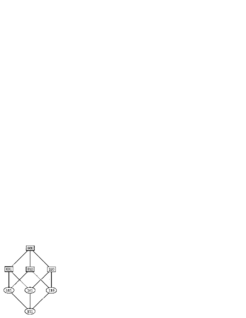
Figure 15: The relationship between the triplet error correction code and active stabilization. The eight possible states of three bits can be placed on the eight corners of a cube, where the sides of the cube connect states which differ by a single bit flip and the two ideal states (000 and 111) lie at opposite corners. Decoding a triplet state by majority vote is equivalent to moving the state to the nearer of the two ideal corners.

Some simple quantum error detection and correction protocols have been implemented on NMR quantum computers Cory:1998b ; Leung:1999 . Full quantum error correction requires at least five qubits to encode a single state, but simpler schemes exist which use only three qubits; these simplified schemes can only correct phase errors or bit-flip errors, but not both. Phase errors occur as a result of spin–spin relaxation, while bit-flip errors correspond to spin–lattice relaxation, and so in many NMR systems phase errors will dominate. Furthermore, phase errors only occur in quantum computers, as they have no classical analogue. For these reasons early studies on NMR error correction have concentrated on three qubit phase-correcting codes.

It should be noted that these NMR experiments are demonstrations of the principle of error correction, rather than practical implementations of error correcting codes. In order to effectively suppress errors in a quantum computation it is necessary to apply the error correction protocol repeatedly; this in turn requires that the ancilla qubits be maintained in the correct state. This is most simply achieved by initialising them to $|0\rangle$ before each correction round. Unfortunately the NMR techniques described in Section VIII allow qubits to be initialised only once, at the start of the calculation; they cannot be repeatedly reinitialised. This appears to rule out current NMR implementations as practical technologies for quantum computation Jones:2000d .

XIII NMR and entanglement

Finally I will return to the question, briefly discussed in Section V, of whether NMR quantum computers are in fact true quantum computers at all. Much of the opposition to NMR as a quantum computing technology stems from the formidable difficulties Jones:2000d in scaling up the current small systems to computers with a reasonable number of qubits. A particularly common observation is that the use of pseudo-pure states is exponentially inefficient Warren:1997 ; Gershenfeld:1997b , in that the amount of pseudo-pure state which can be extracted from an NMR system at thermal equilibrium falls off exponentially with the number of spins in the system. Of course this problem can be overcome by using an exponentially large sample, but this approach would remove any increase in computational efficiency supposedly arising from quantum mechanical effects: there are a wide range of classical techniques (such as DNA computing Adleman:1994 ) which allow exponential gains in computing power to be obtained from exponentially large samples.

This problem is not in principle unique to NMR; it will occur in any potential quantum computing technology which works in the high temperature limit Jones:2000d . It can in principle be overcome by working at sufficiently low temperatures, or by using some other initialisation technique to produce a non-Boltzmann population distribution, although the technical problems involved are substantial Jones:2000d . However NMR is the only technology among those currently under investigation which falls into this category.

In addition to the obvious technological issues raised by this exponential efficiency there are also some more fundamental concerns. It has long been suspected that the non-classical power of quantum computation is closely linked to the existence of entangled states during quantum computations Ekert:1998 . Although this belief has never actually been proved, and some recent theoretical results have suggested that it may not be entirely correct Knill:1998b , it is clear that some important algorithms such as Shor’s quantum factoring algorithm do require the generation of entangled states Linden:1999d . It can be shown that the pseudo-entangled states generated in NMR quantum computations do not actually fulfill the mathematical requirements for true entanglement Braunstein:1999 , casting doubt on their ability to exhibit true quantum phenomena. As we shall see, however, this concern may not be entirely well founded.

XIII.1 Quantifying entanglement

Although the concept of entanglement is relatively easy to explain, actually quantifying the amount of entanglement in any given system is a surprisingly difficult task. For a system of two qubits in a pure state the problem is relatively straightforward, and the four Bell states ($\phi^{\pm}$ and $\psi^{\pm}$, see Section XII) form a basis set describing the possible maximally entangled states. With larger systems the problem is much more difficult, as different definitions of entanglement lead to quite different conclusions.

Difficulties can also arise when considering mixed states, such as those observed in NMR experiments. These difficulties occur because there is no unique way to break down a given mixed state into a mixture of pure states. To see this consider the maximally mixed state, which for a two qubit system has the form

$$\frac{\bm{1}}{4}=\begin{pmatrix}\mbox{$\frac{1}{4}$}&0&0&0\\ 0&\mbox{$\frac{1}{4}$}&0&0\\ 0&0&\mbox{$\frac{1}{4}$}&0\\ 0&0&0&\mbox{$\frac{1}{4}$}\end{pmatrix}.$$ (51)

This is perhaps most easily described as an equally populated mixture of the four eigenstates, but this is by no means the only possible description: an equally weighted mixture of the four Bell states will have exactly the same form! It might be claimed that this alternative decomposition is unnatural, but there are no real grounds for such a statement, as the choice of basis set is entirely arbitrary, and this approach is sometimes referred to as the preferred ensemble fallacy.

Similar difficulties arise when considering the pseudo-entangled states formed from pseudo-pure states, such as

$$(1-\epsilon)\frac{\bm{1}}{4}+\epsilon|\psi^{+}\rangle\langle\psi^{+}|=\begin{pmatrix}\frac{1+\epsilon}{4}&0&0&\frac{\epsilon}{2}\\ 0&\frac{1-\epsilon}{4}&0&0\\ 0&0&\frac{1-\epsilon}{4}&0\\ \frac{\epsilon}{2}&0&0&\frac{1+\epsilon}{4}\end{pmatrix}$$ (52)

(mixed states of this kind were first considered by Werner Werner:1989 , and thus are often referred to as Werner states). It is tempting to argue that this mixed state is a mixture of the maximally mixed state together with a fraction $\epsilon$ of an entangled state, but as discussed above there is no particular reason to choose this description. The amount of apparent entanglement in the state could be increased by decomposing the maximally mixed state as a mixture of entangled states, but it is also possible to choose decompositions which reduce the apparent contribution from entanglement.

While it is not possible to say how much entanglement is in any particular mixed state it is possible to determine the minimum contribution from entangled states which must be present in the state (in a pure entangled state this minimum fraction is, of course, one). If this minimum quantity is greater than zero then it is reasonable to say that the mixed state does contain some entanglement; if, however, the minimum amount is zero then it is possible to describe the mixed state using only product states (and thus without invoking entanglement), and the state is said to be separable. In particular it can be shown Peres:1996 that pseudo-entangled states are in fact separable if $\epsilon<1/3$. An explicit separable decomposition of equation 52 with $\epsilon=1/9$ is given in appendix A.

With larger systems the problem is more complicated, but two important results are known Braunstein:1999 . Given any state $|\psi\rangle$ of an $n$-qubit system, a mixture made by mixing a fraction $\epsilon$ of this state into the maximally mixed state, $\bm{1}/2^{n}$, can always be shown to be separable for sufficiently small values of $\epsilon$, such that

$$\epsilon\leq\frac{1}{1+2^{2n-1}}\sim\frac{2}{4^{n}}.$$ (53)

It can also be shown that non-separable states do exist for sufficiently large values of $\epsilon$, such that

$$\epsilon>\frac{1}{1+2^{n/2}}\sim\frac{1}{2^{n/2}}.$$ (54)

By comparison the values of $\epsilon$ obtainable with NMR quantum computers working within the high temperature limit Jones:2000d ; Warren:1997 ; Gershenfeld:1997b are given by

$$\epsilon\sim\frac{n}{2^{n}}$$ (55)

which lies between the two bounds given in equations 53 and 54. Using realistic parameters it can be calculated that the states used in NMR quantum computations are always separable for systems with less than about $13$ qubits and may (or may not) become entangled beyond this point. Since the systems used so far have involved no more that seven qubits, all NMR quantum computations to date have involved purely separable states.

XIII.2 NMR and quantum mechanics

The observation that NMR quantum computers have so far only used separable states has led some authors to suggest that they are not true quantum computers at all! When assessing claims of this kind it must be remembered that quantum is being used here in its technical sense of provably non-classical. Consider, for example, a set of NMR quantum computers which are identical except for having different values of $\epsilon$, with some of them lying above the entanglement limit discussed previously, and the remainder lying below this limit. It seems very strange to claim that two groups of computers are fundamentally different in character, with the first group being quantum mechanical and the second group classical, but it is more reasonable to suggest that only the computers in the first group are capable of exhibiting convincingly non-classical behaviour.

Even this claim, however, may be too strong. It seems highly unlikely that it is the mere presence of entanglement which leads to non-classical efficiency; rather it is the ability to interconvert a wide range of entangled and non-entangled states. Thus in order to claim that NMR quantum computing experiments are classical it is not sufficient to show that they involve only classical states; instead it is necessary to show that the processes which connect these states can themselves be described classically. To date attempts to achieve this have failed Schack:1999 , and it is not clear that such a model is possible.

In an unrelated approach, some authors have attempted to draw a distinction between the density matrix (which is a description of the state of an NMR system) and the state itself, although it is tricky to draw this distinction in an entirely convincing fashion. It is true, however, that the density matrix approach is only an approximate description of an NMR system, and that any conclusions based on this approximation are to some extent open to suspicion.

XIV Conclusions

When assessing NMR quantum computation it is important to take a balanced view, avoiding both excessive excitement at the apparently impressive results achieved so far and undue despair at the limitations that have been identified. NMR quantum computation has been the subject of a great deal of skeptical scrutiny, probably more than any other approach. In part this is a result of the great success of NMR as a technique for quantum information processing; furthermore, the highly developed nature of NMR experiments, in comparison with many other putative quantum technologies, means that the limits of the technique are well known and understood.

On the positive side, NMR is far ahead of any competing technology in the implementation of quantum computations and other forms of quantum information processing. Although some basic elements have been implemented using other technologies, such as the ion trap controlled-not gate Monroe:1995 , NMR remains the only technology capable of implementing a complete quantum algorithm. Progress from two qubit devices Cory:1996 ; Cory:1997 ; Gershenfeld:1997 ; Jones:1998a ; Chuang:1998a to systems with seven qubits Knill:2000 has been extremely rapid, and there is every reason to believe that more progress will soon be made.

Against this it must be pointed out that most researchers believe that the current designs for NMR quantum computers cannot be extended very much farther: while there is some disagreement as to which technical difficulty will actually stop further progress it is widely agreed that it will be difficult to progress beyond 10–20 qubits. While current demonstration systems are undoubtedly interesting they are far too small to be used to tackle problems beyond the range of current classical computers. Similarly, although there are important applications of quantum information processing, such as quantum cryptography Ekert:2000b , which require only devices with small numbers of qubits, all such applications lie in the field of quantum communication where NMR methods appear completely unsuitable.

The discovery Braunstein:1999 that current NMR implementations of quantum computation do not seem to involve entanglement might appear a serious blow, but its implications should not be overstated. This result does not mean that NMR quantum computers are not true quantum computers, although it does appear to mean that they cannot be used to achieve non-classical efficiencies. However it has long been known Warren:1997 ; Gershenfeld:1997b that the exponential inefficiency of pseudo-pure state preparation means that current implementations are unlikely to exhibit true efficiency gains. It seems likely that in the next few years it will be possible to use para-hydrogen techniques Natterer:1997 ; Duckett:1999 ; Hubbler:2000 to build two qubit NMR quantum computers above the entanglement threshold, but it will be tricky to extend this approach to larger systems.

Appendix A An explicitly separable decomposition of a pseudo-entangled state

While it can be shown that a two qubit pseudo-entangled state with $\epsilon<1/3$ is in fact separable Peres:1996 , the argument used to derive this result does not provide an explicit decomposition of such states into product states, but merely proves that such a decomposition exists. It is, however, fairly simple to find such a decomposition Braunstein:1999 for mixed states with low values of $\epsilon$.

The process begins by constructing an overcomplete basis for a single qubit; a basis set of this kind is sufficient to describe any state of a single qubit (a single spin), but contains more basic elements than is strictly necessary. One suitable basis is the set of six states

$$|0\rangle\quad|1\rangle\quad\frac{|0\rangle\pm|1\rangle}{\sqrt{2}}\quad\frac{|0\rangle\pm i|1\rangle}{\sqrt{2}}$$ (56)

which may be labeled as $\beta_{j}$, $j=1,\,2,\,\dots 6$. This can then be used to construct a two qubit basis set, $\beta_{jk}$, by taking direct products. This basis set, comprising 36 elements, was constructed by taking products of single qubit states, and so is explicitly composed of product states only. Thus any density matrix which can be decomposed in this basis must be separable.

As an example consider a pseudo-entangled state of the form given by equation 52 with $\epsilon=1/9$:

$$\rho=\frac{2}{9}\bm{1}+\frac{1}{9}|\psi^{+}\rangle\langle\psi^{+}|=\frac{1}{18}\begin{pmatrix}5&0&0&1\\ 0&4&0&0\\ 0&0&4&0\\ 1&0&0&5\end{pmatrix}.$$ (57)

This can be written in the form

$$\rho=\sum_{jk}P_{jk}\beta_{jk}$$ (58)

and the proportions $P_{jk}$ of each basis state $\beta_{jk}$ can be obtained from the trace of the product of $\rho$ and $\beta_{jk}$ giving

$$P=\frac{1}{36}\begin{pmatrix}2&0&1&1&1&1\\ 0&2&1&1&1&1\\ 1&1&2&0&1&1\\ 1&1&0&2&1&1\\ 1&1&1&1&0&2\\ 1&1&1&1&2&0\end{pmatrix}.$$ (59)

This calculation also makes clear the danger of an unquestioning equation of entanglement and multiple quantum coherence. The state shown in equation 57 clearly contains double quantum coherence (it can be decomposed in product operator notation as $\mbox{$\frac{1}{2}$}E/2+2I_{z}S_{z}/18+DQ_{x}/9$) and yet is not provably entangled.

References

- (1) C. H. Bennett and D. DiVincenzo, Nature 404 (2000) 247
- (2) C. Macchiavello, G. M. Palma, and A. Zeilinger (Eds.) “Quantum Computation and Quantum Information Theory” (World Scientific, in press).
- (3) D. Bouwmeester, A. Ekert and A. Zeilinger (Eds.) “The Physics of Quantum Information” (Springer-Verlag, Berlin, 2000).
- (4) P. W. Shor, SIAM Review 41 (1999) 303
- (5) R. P. Feynman, Int. J. Theor. Phys. 21 (1982) 467
- (6) S. Lloyd, Science 273 (1996) 1073
- (7) R. R. Ernst, G. Bodenhausen and A. Wokaun, “Principles of Nuclear Magnetic Resonance in One and Two Dimensions” (Oxford University Press, 1987).
- (8) D. G. Cory, A. F. Fahmy and T. F. Havel, in “PhysComp ’96” (T. Toffoli, M. Biafore and J. Leão, Eds.), pp. 87–91, New England Complex Systems Institute (1996)
- (9) D. G. Cory, A. F. Fahmy and T. F. Havel, Proc. Nat. Acad. Sci. USA 94 (1997) 1634
- (10) N. A. Gershenfeld and I. L. Chuang, Science 275 (1997) 350
- (11) J. A. Jones and M. Mosca, J. Chem. Phys. 109 (1998) 1648
- (12) I. L. Chuang, L. M. K. Vandersypen, X. Zhou, D. W. Leung and S. Lloyd, Nature 393 (1998) 143
- (13) J. A. Jones, “NMR Quantum Computing”, in reference Macchiavello:2000 .
- (14) J. A. Jones, “Quantum Computing and NMR”, in reference Bouwmeester:2000 .
- (15) R. P. Feynman, “Feynman Lectures on Computation”, edited by A. J. G. Hey and R. W. Allen (Addison-Wesley, Reading, MA, 1996).
- (16) O. W. Sørensen, G. W. Eich, M. H. Levitt, G. Bodenhausen and R. R. Ernst, Prog. NMR. Spectrosc. 16 (1983) 163
- (17) M. Goldman, “Quantum Description of High-Resolution NMR in Liquids” (Clarendon Press, Oxford, 1988).
- (18) http://www.arxiv.org/quant-ph
- (19) M. Schulz, Nature 399 (1999) 729
- (20) D. Welsh, “Codes and Cryptography” (Clarendon Press, Oxford, 1988).
- (21) B. Schneier, “Applied Cryptography” (John Wiley, 1996).
- (22) D. Deutsch, Proc. R. Soc. Lond. A 400 (1985) 97
- (23) D. Deutsch, in “Quantum Concepts in Space and Time” (R. Penrose and C. J. Isham, Eds.), (Clarendon Press, Oxford, 1986).
- (24) D. Deutsch and R. Jozsa, Proc. R. Soc. Lond. A 439 (1992) 553
- (25) R. Cleve, A. Ekert, C. Macchiavello and M. Mosca, Proc. R. Soc. Lond. A 454 (1998) 339
- (26) A. Ekert and R. Jozsa, Rev. Mod. Phys. 68 (1996) 733
- (27) C. H. Bennett, IBM J. Res. Dev 17 (1973) 525
- (28) E. Fredkin and T. Toffoli, Int. J. Theor. Phys. 21 (1982) 219
- (29) R. Landauer, IBM J. Res. Dev. 5 (1961) 183
- (30) R. Landauer, Int. J. Theor. Phys. 21 (1982) 283
- (31) D. P. DiVincenzo, Proc. R. Soc. Lond. A 454 (1998) 261
- (32) D. Deutsch, Proc. R. Soc. Lond. A 425 (1989) 73
- (33) A. Barenco, C. H. Bennett, R. Cleve, D. P. DiVincenzo, N. Margolus, P. Shor, T. Sleator, J. Smolin and H. Weinfurter, LANL e-print quant-ph/9503016.
- (34) A. Barenco, Proc. R. Soc. Lond. A 449 (1995) 679
- (35) D. Deutsch, A. Barenco and A. Ekert, Proc. Roy. Soc. Lond. A 449 (1995) 669
- (36) S. Lloyd, Phys. Rev. Lett. 92 (1995) 346
- (37) D. P. DiVincenzo, Fort. der Physik, in press. See also LANL e-print quant-ph/0002077.
- (38) J. A. Jones, Fort. der Physik, in press. See also LANL e-print quant-ph/0002085.
- (39) T. G. Walker and W. Happer, Rev. Mod. Phys. 69 (1997) 629
- (40) G. Navon, Y. Q. Song, T. Rõõm, A. Appelt, R. E. Taylor and A. Pines, Science 271 (1996) 1848
- (41) T. Pietraß, Coll. Surf. A 158 (1999) 51
- (42) J. Natterer and J. Bargon, Prog. NMR Spectrosc. 31 (1997) 293
- (43) S. B. Duckett and C. J. Sleigh, Prog. NMR Spectrosc. 34 (1999) 71
- (44) P. Hübbler, J. Bargon and S. J. Glaser, J. Chem. Phys., in press.
- (45) R. Freeman, “Spin Choreography” (Spektrum, Oxford, 1997).
- (46) W. S. Warren, Science 277 (1997) 1688
- (47) N. A. Gershenfeld and I. L. Chuang, Science 277 (1997) 1689
- (48) J. A. Jones, R. H. Hansen and M. Mosca, J. Magn. Reson. 135 (1998) 353
- (49) R. Freeman, T. A. Frenkiel and M. H. Levitt, J. Magn. Reson. 44 (1981) 409
- (50) J. A. Jones and E. Knill, J. Magn. Reson. 141 (1999) 322
- (51) D. W. Leung, I. L. Chuang, F. Yamaguchi and Y. Yamamoto, Phys. Rev. A 61 (2000) 042310
- (52) N. Linden, Ē. Kupc̆e and R. Freeman, Chem. Phys. Lett. 311 (1999) 321
- (53) Z. L Mádi, R. Brüschweiler and R. R. Ernst, J. Chem. Phys. 109 (1998) 10603
- (54) N. Linden, H. Barjat, Ē. Kupc̆e and R. Freeman, Chem. Phys. Lett. 307 (1999) 198
- (55) M. D. Price, S. S. Somaroo, A. E. Dunlop, T. F. Havel and D. G. Cory, Phys. Rev. A 60 (1999) 2777
- (56) M. D. Price, T. F. Havel and D. G. Cory, New. J. Phys. 2.10 (2000) 1
- (57) A. Barenco, D. Deutsch, A. Ekert and R. Jozsa, Phys. Rev. Lett. 74 (1995) 4083
- (58) N. Linden, H. Barjat and R. Freeman, Chem. Phys. Lett. 296 (1998) 61
- (59) K. G. R. Pachler and P. L. Wessels, J. Magn. Reson. 12 (1973) 337
- (60) G. A. Morris and R. Freeman, J. Am. Chem. Soc. 101 (1979) 760
- (61) K. Dorai, Arvind and A. Kumar, Phys. Rev. A 61 (2000) 042306
- (62) J. A. Jones, V. Vedral, A. Ekert and G. Castagnoli, Nature 403 (2000) 869
- (63) A. Ekert, M. Ericsson, P. Hayden, H. Inamori, J. A. Jones, D. L. K. Oi and V. Vedral, J. Mod. Opt (in press).
- (64) A. Shapere and F. Wilczek, “Geometric Phases in Physics” (World Scientific, Singapore, 1989).
- (65) M. V. Berry, Proc. Roy. Soc. Lond. A 392 (1984) 45
- (66) D. Suter, G. Chingas, R. Harris and A. Pines, Molec. Phys. 61 (1987) 1327
- (67) M. Goldman, V. Fleury and M. Guéron, J. Magn. Reson. A 118 (1996) 11
- (68) R. Tycko, Phys. Rev. Lett. 58 (1987) 2281
- (69) S. Appelt, G. Wäckerle and M. Mehring, Phys. Rev. Lett. 72 (1994) 3921
- (70) J. A. Jones and A. Pines, J. Chem. Phys. 106 (1997) 3007
- (71) E. Knill, I. Chuang and R. Laflamme, Phys. Rev. A 57 (1998) 3348
- (72) E. Knill, R. Laflamme, R. Martinez and C.-H. Tseng, Nature 404 (2000) 368
- (73) M. Pravia, E. Fortunato, Y. Weinstein, M. D. Price, G. Teklemariam, R. J. Nelson, Y. Sharf, S. Somaroo, C. H. Tseng, T. F. Havel and D. G. Cory, Concepts Magn. Reson. 11 (1999) 225
- (74) L. M. K. Vandersypen, C. S. Yannoni, M. H. Sherwood and I. L. Chuang, Phys. Rev. Lett. 83 (1999) 3085
- (75) R. Marx, A. F. Fahmy, J. M. Myers, W. Bermel and S. J. Glaser, Phys. Rev. A, 62 (2000) 012310
- (76) D. Bouwmeester and A. Zeilinger, “The Physics of Quantum Information: Basic Concepts”, in reference Bouwmeester:2000 .
- (77) I. L. Chuang, N. Gershenfeld and M. Kubinec, Phys. Rev. Lett. 80 (1998) 3408
- (78) P. Plateau and M. Guéron, J. Am. Chem. Soc. 104 (1982) 7310
- (79) J. A. Jones and M. Mosca, Phys. Rev. Lett. 83 (1999) 1050
- (80) M. H. Levitt, Prog. NMR Spectrosc. 18 (1986) 61
- (81) H. K. Cummins and J. A. Jones, New J. Phys 2.6 (2000) 1
- (82) R. Tycko, Phys. Rev. Lett. 51 (1983) 775
- (83) H. K. Cummins and J. A. Jones, submitted to J. Magn. Reson. See also LANL e-print quant-ph/0008034.
- (84) D. Collins, K. W. Kim and W. C. Holton, Phys. Rev. A 58 (1998) R1633
- (85) D. Collins, K. W. Kim, W. C. Holton, H. Sierzputowska-Gracz and E. O. Stejskal, Phys. Rev. A 62 (2000) 022304.
- (86) Arvind, K. Dorai and A. Kumar, LANL e-print quant-ph/9909067.
- (87) L. K. Grover, Phys. Rev. Lett. 79 (1997) 325
- (88) L. K. Grover, Science 280 (1998) 228
- (89) J. A. Jones, M. Mosca and R. H. Hansen, Nature 393 (1998) 344
- (90) J. A. Jones Science 280 (1998) 229
- (91) L. M. K. Vandersypen, M. Steffen, M. H. Sherwood, C. S. Yannoni, G. Breyta and I. L. Chuang, Appl. Phys. Lett. 76 (2000) 646
- (92) M. Boyer, G. Brassard, P. Høyer and A. Tapp, Fort. Der. Physik 46 (1998) 493
- (93) G. Brassard, P. Høyer and A. Tapp, Proceedings of ICALP 1998; see also LANL e-print quant-ph/9805082.
- (94) M. Mosca, Proceedings of Randomized Algorithms 1998.
- (95) R. Laflamme, E. Knill, W. H. Zurek, P. Catasti and S. V. S. Mariappan, Phil. Trans. R. Soc. Lond A 356 (1998) 1941
- (96) D. Bouwmeester, J.-W. Pan, M. Daniell, H. Weinfurter and A. Zeilinger, Phys. Rev. Lett. 82 (1999) 1345
- (97) L. Emsley and A. Pines “Lectures on Pulsed NMR”, in B. Maraviglia (Ed.) “Proceedings of the International School of Physics ‘Enrico Fermi’ ” (Società Italiana di Fisica, 1992).
- (98) D. Bouwmeester, H. Weinfurter and A. Zeilinger, “Quantum Dense Coding and Quantum Teleportation”, in reference Bouwmeester:2000 .
- (99) C. H. Bennett, G. Brassard, C. Crépeau, R. Jozsa, A. Peres and W. K. Wooters, Phys. Rev. Lett. 70 (1993) 1895
- (100) D. Bouwmeester, J.-W. Pan, K. Mattle, M. Eible, H. Weinfurter and A. Zeilinger, Nature 390 (1997) 575
- (101) M. A. Nielsen, E. Knill and R. Laflamme, Nature 396 (1998) 52
- (102) P. W. Shor, Phys. Rev. A 52 (1995) 2493
- (103) A. M. Steane, Phys. Rev. Lett. 77 (1996) 793
- (104) A. M. Steane, Phil. Trans. Roy. Soc. Lond. A 356 (1998) 1739
- (105) A. M. Steane, Nature 399 (1999) 6732
- (106) D. G. Cory, M. D. Price, W. Maas, E. Knill, R. Laflamme, W. H. Zurek, T. F. Havel and S. S. Somaroo, Phys. Rev. Lett. 81 (1998) 2152
- (107) D. Leung, L. Vandersypen, X. L. Zhou, M. Sherwood, C. Yannoni, M. Kubinec and I. Chuang Phys. Rev. A 60 (1999) 1924
- (108) L. M. Adleman, Science 266 (1994) 1021
- (109) A. Ekert and R. Jozsa, Phil. Trans. Roy. Soc. Lond. A 356 (1998) 1769
- (110) E. Knill and R. Laflamme, Phys. Rev. Lett. 81 (1998) 5672
- (111) N. Linden and S. Popescu, LANL e-print quant-ph/9906008.
- (112) S. L. Braunstein, C. M. Caves, R. Jozsa, N. Linden, S. Popescu, R. Schack, Phys. Rev. Lett. 83 (1999) 1054
- (113) R. F. Werner, Phys. Rev. A 40 (1989) 4276
- (114) A. Peres, Phys. Rev. Lett. 77 (1996) 1412
- (115) R. Schack and C. M. Caves, Phys. Rev. A 60 (1999) 4354
- (116) C. Monroe, D. M. Meekhof, B. E. King, W. M. Itano and D. J. Wineland, Phys. Rev. Lett. 75 (1995) 4714
- (117) A. Ekert, N. Gisin, B. Huttner, H. Inamori, and H. Weinfurter, “Quantum Cryptography”, in reference Bouwmeester:2000 .