Dagomir Kaszlikowski

Nonclassical Phenomena

in Multi-photon Interferometry:

More Stringent Tests Against Local Realism

Abstract

The present dissertation consists of three parts which are mainly based on the following papers:

• M. Żukowski, D. Kaszlikowski and E. Santos, Phys. Rev. A 60, R2614 (1999)

• M. Żukowski and D. Kaszlikowski, Acta Phys. Slov. 49, 621 (1999)

• M. Żukowski and D. Kaszlikowski, Phys. Rev. A 56, R1682 (1997)

• D. Kaszlikowski and M. Żukowski, Phys. Rev. A 61, 022114 (2000)

• M. Żukowski and D. Kaszlikowski, Phys. Rev. A 59, 3200 (1999)

• M. Żukowski and D. Kaszlikowski, Vienna Circle Yearbook vol. 7, editors D. Greenberger, W. L. Reiter, A. Zeilinger, Kluwer Academic Publishers, Dortrecht (1999)

• M. Żukowski, D. Kaszlikowski, A. Baturo and J. -Å. Larsson, quant-ph/9910058

• D. Kaszlikowski, P. Gnacinski, M. Żukowski, W. Miklaszewski and A. Zeilinger, quant-ph/0005028

The first two chapters have an introductory character.

In Chapter 3 it is shown [1] that the possibility of distinguishing between single- and two- photon detection events, usually not met in the actual experiments, is not a necessary requirement for the proof that the experiments of Alley and Shih [Shih88] and Ou and Mandel [Ou88] are, modulo a fair sampling assumption, valid tests of local realism. It is also shown that some other interesting phenomena (involving bosonic-type particle indistinguishability) can be observed during such tests.

Next in Chapter 4 it is shown again [2] that the possibility of distinguishing between single and two photon detection events is not a necessary requirement for the proof that recent operational realisation of entanglement swapping cannot find a local realistic description. A simple modification of the experiment is proposed, which gives a richer set of interesting phenomena.

In Chapter 5 a sequence of Bell inequalities for $M$ particle systems, which involve three settings of each of the local measuring apparatuses, is derived [3]. For Greenberger-Horne-Zeilinger states, quantum mechanics violates these inequalities by factors exponentially growing with $M$. The threshold visibilities of the multiparticle sinusoidal interference fringes, for which local realistic theories are ruled out by these inequalities, decrease as $(2/3)^{M}$.

In Chapter 6 the Bell theorem for a pair of two two-state systems (qubits) in a singlet state for the entire range of measurement settings is presented [4].

Chapter 7 is devoted to derivation of a series of Greenberger-Horne-Zeilinger paradoxes for $M$ qu$N$its (particles described by an $N$ dimensional Hilbert space) that are fed into $M$ unbiased $2N$-port spatially separated beam splitters [5, 6].

In Part III a novel approach to the Bell theorem, via numerical linear optimisation, is presented [7, 8].

The two-qubit correlation obtained from the quantum state used in the Bell inequality is sinusoidal, but the standard Bell inequality only uses two pairs of settings and not the whole sinusoidal curve. The highest to-date visibility of an explicit model reproducing sinusoidal fringes is ${2\over\pi}$. We conjecture from a numerical approach [7] presented in Chapter 8 that the highest possible visibility for a local hidden variable model reproducing the sinusoidal character of the quantum prediction for the two-qubit Bell-type interference phenomena is ${1\over\sqrt{2}}$. In addition, the approach can be applied directly to experimental data.

In Chapter 9 the approach presented in Chapter 8 is applied to three qubits in a maximally entangled Greenberger-Horne-Zeilinger state. For the first time the necessary and sufficient conditions for violation of local realism for the case in which each observer can choose from up to 5 settings of the measuring apparatus are shown.

In Chapter 10 using the modified approach developed in Chapter 8 it is shown that violations of local realism are stronger for two maximally entangled qu$N$its, than for two qubits [8]. The magnitude of violation increases with $N$. It is objectively defined by the required minimal admixture of pure noise to the maximally entangled state such that a local realistic description is still possible. Operational realisation of the two qu$N$it measurement exhibiting strong violations of local realism involves entangled photons and unbiased multiport beamsplitters. The approach, extending at present to $N=9$, neither involves any simplifications, or additional assumptions, nor does it utilise any symmetries of the problem.

Contents

1. 1 Introduction
2. 2 Some history and basic notions
   1. 2.1 Preliminaries
   2. 2.2 Entanglement
   3. 2.3 Elements of reality
   4. 2.4 The Bell theorem
   5. 2.5 Experimental tests of the Bell theorem
      1. 2.5.1 First experiments
      2. 2.5.2 New experiments
      3. 2.5.3 Problems encountered in the Bell type experiments
3. I New theoretical analysis of Alley-Shih, Ou-Mandel and entanglement swapping experiments
   1. 3 Alley-Shih and Ou-Mandel experiments: resolution of the problem of distinguishability of single and two photon events [1]
      1. 3.1 Introduction
      2. 3.2 Description of the experiment
      3. 3.3 Quantum predictions
      4. 3.4 Conditions to violate local realism
      5. 3.5 Conclusions
   2. 4 Better entanglement swapping [2]
      1. 4.1 Introduction
      2. 4.2 Description of the experiment
      3. 4.3 Quantum predictions
      4. 4.4 Conditions to violate local realism
      5. 4.5 Proposal of modification of the experiment
      6. 4.6 Conclusions
4. II New generalised Bell inequalities and GHZ paradoxes for qu$N$its
   1. 5 Wringing out better Bell inequalities for GHZ experiment [3]
      1. 5.1 Introduction
      2. 5.2 Geometrical method of finding Bell inequalities
      3. 5.3 Quantum and local realistic description of the gedanken experiment
      4. 5.4 Derivation of Bell inequalities via the geometrical method
         1. 5.4.1 Critical visibility and quantum efficiency of detectors
      5. 5.5 Results
      6. 5.6 Conclusions
   2. 6 Bell inequality for all possible local settings [4]
      1. 6.1 Introduction
      2. 6.2 Quantum mechanical and local realistic description of the gedanken experiment
      3. 6.3 Derivation of the inequality via the geometrical method
      4. 6.4 Results
      5. 6.5 Conclusions
   3. 7 Greenberger-Horne-Zeilinger paradoxes for qu$N$its [5,6]
      1. 7.1 Introduction
      2. 7.2 Unbiased multiport beamsplitters
      3. 7.3 Quantum mechanical predictions
         1. 7.3.1 Bell number assignment
         2. 7.3.2 Perfect correlations
      4. 7.4 Paradoxes for $N+1$ maximally entangled qu$N$its
         1. 7.4.1 Four tritters
         2. 7.4.2 General case: $N+1$ maximally entangled qu$N$its
      5. 7.5 Paradoxes for $N$ maximally entangled qu$N$its.
         1. 7.5.1 Three tritters
         2. 7.5.2 General case: N maximally entangled qu$N$its.
      6. 7.6 Conclusions
5. III Extension of Bell Theorem via numerical approach
   1. 8 Necessary and sufficient conditions to violate local realism for two maximally entangled qubits- extension to more than two local settings [7]
      1. 8.1 Introduction
      2. 8.2 Quantum mechanical and local realistic description of the gedanken experiment
      3. 8.3 Linear programming and Downhill Simplex Method
         1. 8.3.1 Numerical difficulties
      4. 8.4 Results
         1. 8.4.1 Exemplary numerical model
      5. 8.5 Application to experimental data
      6. 8.6 Conclusions
   2. 9 Necessary and sufficient conditions to violate local realism for three maximally entangled qubits- extension to more than two local settings
      1. 9.1 Description of the method
      2. 9.2 Results
      3. 9.3 Conclusions
   3. 10 Entangled pairs of qu$N$its: the violation of local realism increases with $N$ [8]
      1. 10.1 Introduction
      2. 10.2 Description of the gedanken experiment
      3. 10.3 Local realism and joint probability distribution
      4. 10.4 Linear programming
      5. 10.5 Observables
      6. 10.6 Results
      7. 10.7 Exemplary analytical model for $N=3$
         1. 10.7.1 Explicit model for extremal case
      8. 10.8 Conclusions
   4. A Proof of equivalence of the existence of local hidden variables and a joint probability distribution for incompatible measurements

Chapter 1 Introduction

Bell’s theorem [Bell64], formulated in 1964, initiated and revitalised several branches of modern physics. The paper was the first one to show that quantum entanglement cannot be in any way simulated by classical correlations. Within few years, a new branch of experimental physics emerged: multi-particle quantum interferometry. Since then it has evolved and extended its field of interest from two-photon to multi-photon correlations. Recently Bell-EPR correlations were observed for entangled atoms [Hagley97]. For as much as nearly 20-25 years the paper of Bell was studied mainly by people interested in the foundational-interpretational problems of quantum theory. Suddenly with the discovery of the possibility of employing Bell-EPR correlations [Eckert91] in ”quantum cryptography” [Bennett84] and with the realisation of the importance of entanglement in the hypothetical quantum computers [Feynman82, Deutsch89], it turned out that the paper of Bell can be thought of as the first one in the field of quantum information.

Studies of quantum information led to a proposal, employing entanglement, of quantum teleportation [Bennett93]. This phenomenon was observed in 1997 and seems to be at the moment the crowning achievement of quantum interferometry [Bouwmeester97]. Interestingly, the method to obtain quantum teleportation of photon’s polarisation was developed independently, as a by product of theoretical and experimental research towards obtaining Bell-EPR phenomena for particles originating from independent sources [Yurke92, Żukowski93a, Pan98].

The same method was applied to obtain the first ever observations of Greenberger-Horne-Zeilinger correlations (GHZ) [Bouwmeester99]. The 1989 theoretical discovery of GHZ correlations [Greenberger89] and the drastic amplification of the Bell theorem, which is implied by them, was the event in the research into foundations of quantum theory which amplified interest in entanglement (with the interesting sociological consequence: the earlier terminology- correlated state- was replaced by the Schrödinger’s term entanglement).

The technological progress of 1980’s and 1990’s has enabled all that experimental and theoretical activity to flourish. The phenomenon of parametric down conversion (PDC) turned out to be a versatile source of entangled photons. The simplicity of the phenomenon of PDC has lead to an explosion of the number of experiments studying various aspects of entanglement or the basic phenomena linked with quantum information and quantum communication (dense coding [Mattle96], Bell-state measurement [Michler96], etc.). Pulsed down conversion enabled to observe two-photon interferometric effect for independently emitted photons [Pan98]. The future of experimental quantum information most probably will be associated with trapped atoms and microcavity-atom interactions [Hagley97]- fields in which extensive studies of entanglement are currently carried out.

Interestingly, all these developments led to studies concerning entanglement properties of mixed states. In the case of the Bell theorem the pioneering works were by Werner (1989) [Werner89] and the Horodecki Family (1995) [Horodecki95]. In recent years one observes an avalanche of works on the problem of separability of density matrices initialised by Peres [Peres96] and again the Horodecki Family (see e.g. [Horodecki96]). The research into the separability has shown once more (recall Bell-Kochen-Specker theorem [Kochen67]) the qualitative difference between systems described by 2-dimensional Hilbert space (qubits) and those described by Hilbert spaces of higher dimension (qu$N$its).

The present work tries to answer some questions on the relation of the Bell theorem with various performed or proposed multiparticle (essentially, multiphoton) quantum interference experiments.

The first part deals with some of performed experiments. Proposals of improvements and re-interpretations are given [1, 2].

Next, in part two, we study new methods of deriving Bell inequalities both for the standard two qubit experiments as well as to multi-qubit GHZ experiments [3, 4]. Derivation of GHZ paradoxes for gedanken experiments involving $M$ entangled qu$N$its observed beyond multiport beamsplitters [Żukowski97b] is also shown [5, 6].

Finally the last part is devoted to the Bell theorem without inequalities via a numerical approach utilising linear optimisation [7, 8].

Chapter 2 Some history and basic notions

2.1 Preliminaries

According to a prevailing common opinion quantum mechanics is a fundamental theory which applies to all physical systems. Its predictive power is astonishing. Up to the present day there has not been a single experiment which invalidates it. However, the conclusions that can be drawn from quantum mechanics force us to entirely abandon the picture of nature implied by classical physics and the common sense. One of the main sources of difference between the quantum world and the classical one, in which we are particularly interested in this work, is entanglement.

The notion of entanglement was introduced for the first time by Schrödinger to describe a situation in which

Maximal knowledge of a total system does not necessarily include total knowledge of all its parts, not even when these are fully separated from each other and at the moment are not influencing each other at all…

The work of Schröedinger [Schröedinger35] was partially motivated by the seminal paper of Einstein, Podolsky and Rosen (EPR) [Einstein35] in which the authors used an entangled state (an EPR state) of two qubits to show that quantum mechanics could not be considered as a complete physical theory aiming to describe the phenomena occurring in micro world. Although they did not state it clearly, EPR effectively postulated the existence of local hidden variables, in the form of ”elements of reality”, which were to play the same role in quantum mechanics as the positions and velocities of particles in statistical classical mechanics and that were to solve the interpretational problems of quantum mechanics. That paper directly influenced the formulation of the Bell theorem [Bell64, Bell66, Bell87].

In his 1964 paper Bell for the very first time showed that the idea of local hidden variables was in contradiction with quantum mechanics and, what is even more important, that it could be tested experimentally! That way the subject mainly discussed by physicists at the parties was brought to the realm of experimentally verifiable physics.

2.2 Entanglement

To discuss basic features of entanglement let us consider the following state of two two-state systems (qubits)

$$|\psi\rangle={1\over\sqrt{2}}(|0\rangle_{1}\otimes|1\rangle_{2}-|1\rangle_{1}\otimes|0\rangle_{2}),$$ (2.1)

where $\otimes$ denotes the tensor product and kets $|0\rangle_{i},|1\rangle_{i}$ describe two orthogonal states of the $i$-th qubit. The above pure state describes a coherent superposition of two product states that occur with equal probability.

According to quantum mechanics $|\psi\rangle$ contains all available information about the state of the qubits. If we write (2.1) in the form of a density matrix $\rho_{12}$

$$\rho_{12}=|\psi\rangle\langle\psi|={1\over 2}\left[|0\rangle_{1}{}_{1}\langle 0|\otimes|1\rangle_{2}{}_{2}\langle 1|-|0\rangle_{1}{}_{1}\langle 1|\otimes|1\rangle_{2}{}_{2}\langle 0|\right.$$

$$\left.-|1\rangle_{1}{}_{1}\langle 0|\otimes|0\rangle_{2}{}_{2}\langle 1|+|1\rangle_{1}{}_{1}\langle 1|\otimes|0\rangle_{2}{}_{2}\langle 0|\right],$$ (2.2)

and trace out one qubit we obtain a density matrix describing the other qubit, which reads

$$\rho_{k}={1\over 2}\left(|1\rangle_{k}{}_{k}\langle 1|+|0\rangle_{k}{}_{k}\langle 0|\right),$$ (2.3)

$k=1,2$. Such a density matrix describes a situation in which we have a chaotic mixture of two orthogonal pure states. This is a situation typical for the entanglement. We have the full possible information about the state of two qubits as a whole but we do not have any information about the state of each qubit separately, which in fact is not even defined! In addition, the properties of the qubits are tightly correlated.

To see this more clearly let us consider the measurement of two dichotomic observables with spectrum consisting of $\pm 1$, which spectral decomposition has the following form

$$\hat{O}_{k}(\phi_{k})=|+,\phi_{k}\rangle_{k}{}_{k}\langle+,\phi_{k}|-|-,\phi_{k}\rangle_{k}{}_{k}\langle-,\phi_{k}|$$ (2.4)

with $k=1,2$ and

$$|+,\phi_{k}\rangle_{k}={1\over\sqrt{2}}\left(|0\rangle_{k}+e^{i\phi_{k}}|1\rangle_{k}\right)$$

$$|-,\phi_{k}\rangle_{k}={1\over\sqrt{2}}\left(|0\rangle_{k}-e^{i\phi_{k}}|1\rangle_{k}\right),$$ (2.5)

where $\phi_{k}\in[0,2\pi]$. The mean value $E_{QM}(\phi_{1},\phi_{2})$ of the joint measurement of the observable $\hat{O}_{1}(\phi_{1})$ on the first qubit and the observable $\hat{O}_{2}(\phi_{2})$ on the second one- the so called correlation function- reads

$$E_{QM}(\phi_{1},\phi_{2})=\langle\psi|\hat{O}_{1}(\phi_{1})\hat{O}_{2}(\phi_{2})|\psi\rangle=-\cos(\phi_{1}+\phi_{2}).$$ (2.6)

It is easy to see that, for example, whenever the sum of the phases $\phi_{1}$ and $\phi_{2}$ is $0$ modulo $2\pi$ we observe the so called perfect correlations between the results of the measurements performed by the observers; if the first observer obtains $+1$ as the result of his measurement the second one obtains $-1$ and vice versa. However, each observer alone measures $+1$ and $-1$ with equal probability, which can be easily seen using the density matrix (2.3)

$$\langle O_{k}(\phi_{k})\rangle_{\rho_{k}}=Tr(O_{k}(\phi_{k})\rho_{k})=0.$$ (2.7)

The above formulas clearly demonstrate that all information about the state (2.1) is contained in the joint properties of the qubits.

2.3 Elements of reality

In their famous paper [Einstein35] EPR used the perfect correlations observed when measuring local observables on an entangled system of spatially separated qubits (2.1) to demonstrate that quantum mechanics is incomplete, i.e., that one needs some additional parameters to fully describe phenomena occurring in micro world. We briefly present their reasoning in the version of Bohm [Bohm51, Bohm52] to introduce the notion of local realism, which plays a central part in the Bell theorem.

EPR reasoning goes as follows. According to quantum mechanics all we know about the system of two entangled qubits is encoded in the state (2.1). Quantum mechanics also tells us that we cannot consider simultaneous measurements of two non commuting observables and therefore does not even define predictions for such cases. Let us imagine that the observers one and two are spatially separated and that they simultaneously measure the observables $\hat{O}_{1}(\phi_{1}=0)$ and $\hat{O}_{2}(\phi_{2}=0)$ (see the picture (2.1)) on subsystems described by the singlet state.

Figure 2.1: The scheme of the Bell type experiment. Solid arrows represent actual positions of the measuring apparatus, dashed arrow the future ones. Detectors $A_{1},A_{2},B_{1},B_{2}$ register incoming qubits.

For such observables the perfect correlations occur, which means that if the first observer has obtained $+1$ the second one, because of (2.6), must have obtained $-1$ and vice versa. Moreover, due to the spatial separation of the observers and the non superluminal velocity of propagation of any interaction (information) in nature (locality), the outcome of the first (second) observer cannot be influenced by the choice of observable measured by the second (first) observer and neither by its outcome. All correlations between the results of measurements must have been established in the source.

However, the second observer could have measured the observable $\hat{O}_{2}(\phi_{2}^{\prime}={\pi\over 2})$ instead of the previous one characterised by $\phi_{2}=0$. Then, the result of this would-be measurement, would have enabled him to infer with probability equal to one and without disturbing the first qubit the result of the measurement of the observable $\hat{O}_{1}(\phi_{1}^{\prime}={\pi\over 2})$ by the first observer. At this stage of reasoning EPR introduce the notion of physical reality [Einstein35]:

If, without in any way disturbing a system, we can predict with certainty (i.e. with probability equal to unity) the value of a physical quantity, then there exists an element of physical reality corresponding to this physical quantity.

According to this definition the inference made by the second observer about the result of the measurement that could have been made by the first observer has a well defined physical meaning. This would mean that it is possible to ascribe the definite values to the results of the measurement of two non commuting observables $\hat{O}_{i}(\phi_{i}=0)$ and $\hat{O}_{i}(\phi_{i}^{\prime}={\pi\over 2})$ ($i=1,2$), the statement which makes quantum purist’s hair stand on ends. Therefore, according to EPR, quantum mechanics is incomplete and should be completed at least by introducing elements of reality into the description of quantum state.

2.4 The Bell theorem

The hypothesis of local hidden variables, which effectively stems from the notion of elements of reality, was proved to be unacceptable for systems described by quantum mechanics by Bell, [Bell64] who found an inequality which should be obeyed by any local hidden variable theory, and which is violated by predictions of quantum mechanics. Here we present the derivation of the Clauser-Horne-Shimony-Holt (CHSH) inequality [Clauser69].

To this end, let us again consider the experiment in which two spatially separated observers perform the measurements of the observables defined in (2.4) on the state (2.1). Each of them as a result of their measurement obtains only one of the two possible values $\pm 1$ (they measure bivalued observables). Although the different results of the measurement at each observer’s side occur with equal probability the results of joint measurements are correlated, which is expressed by the formula (2.6). If deterministic local hidden variables exist they predetermine the results of each single measurement for each observer at the time of the emission of each pair of qubits. In other words, the value of the local hidden variable for a particular emission of a pair of qubits would allow us to predict the result of the measurement made by each observer with certainty. However this value is hidden. To model the probabilistic nature of quantum experiments we assume that there exists some probability distribution of local hidden variables associated with a given quantum mechanical state, which represents our lack of knowledge about them.

To express the above idea of local hidden variables mathematically we assume that there is a set of hidden variables $\Lambda$ on which we can define a probabilistic measure $d\rho(\lambda)$. We also assume the existence of two bivalued functions $O_{1},O_{2}$ defined on the space $\Lambda$ which take only the values $\pm 1$. Each of these two functions must depend on the local parameters $\phi_{1}$ and $\phi_{2}$ characterising the experiment performed by the first and the second observer respectively. Because of the assumption of locality the function $O_{1}$ can solely depend on the $\phi_{1}$ and the other one on $\phi_{2}$. Thus, the correlation function based on the idea of local hidden variables must have the following form

$$E_{LHV}(\phi_{1},\phi_{2})=\int_{\Lambda}d\rho(\lambda)O_{1}(\lambda,\phi_{1})O_{2}(\lambda,\phi_{2}),$$ (2.8)

where $\int_{\Lambda}d\rho(\lambda)=1$.

Now, let us imagine that each observer performs two mutually exclusive experiments characterised by $\phi_{i},\phi_{i}^{\prime}$ and let us consider the following expression made out of the four local hidden variables correlation functions (2.8)

$$C_{LHV}=E_{LHV}(\phi_{1},\phi_{2})+E_{LHV}(\phi_{1}^{\prime},\phi_{2})+E_{LHV}(\phi_{1},\phi_{2}^{\prime})-E_{LHV}(\phi_{1}^{\prime},\phi_{2}^{\prime})$$

$$=\int_{\Lambda}d\rho(\lambda)\left[O_{1}\left(\lambda,\phi_{1})(O_{2}(\lambda,\phi_{2})+O_{2}(\lambda,\phi_{2}^{\prime})\right)+O_{1}(\lambda,\phi_{1}^{\prime})\left(O_{2}(\lambda,\phi_{2})-O_{2}(\lambda,\phi_{2}^{\prime})\right)\right].$$ (2.9)

It is easy to see that the modulus of the expression in the square brackets is either $-2$ or $+2$. Therefore, the hypothesis of local hidden variables implies that the following inequality (Bell-CHSH inequality) must be valid

$$-2\leq C_{LHV}\leq 2.$$ (2.10)

Is the CHSH inequality always satisfied by quantum predictions for (2.1)? To answer this question let us put $\phi_{1}=0,\phi_{1}^{\prime}={\pi\over 2}$ and $\phi_{2}=-\pi/4,\phi_{2}^{\prime}=\pi/4$. For these values of local parameters one has

$$C_{QM}=E_{QM}(\phi_{1},\phi_{2})+E_{QM}(\phi_{1}^{\prime},\phi_{2})+E_{QM}(\phi_{1},\phi_{2}^{\prime})-E_{QM}(\phi_{1}^{\prime},\phi_{2}^{\prime})$$

$$=-\cos(\phi_{1}+\phi_{2})-\cos(\phi_{1}^{\prime}+\phi_{2})-\cos(\phi_{1}+\phi_{2}^{\prime})+\cos(\phi_{1}^{\prime}+\phi_{2}^{\prime})=-2\sqrt{2}.$$ (2.11)

Because $-2\sqrt{2}<-2$, we have a contradiction.

The above result, known as the Bell theorem, needs some further explanation. In our reasoning we have made two crucial assumptions without which the theorem would not be valid. These assumptions are: locality and realism. The Bell theorem tells us that either notion of locality, or realism, or both are false in quantum theory [Redhead87].

Another remark is that the Bell-CHSH inequality can be directly applied to any experimental data. Also, even if quantum mechanics is not valid and we will find another better theory we can still, using the Bell inequality, verify whether this new theory fulfils the necessary condition for the local realistic description or not.

The final remark is that one may consider the existence of the so called stochastic local hidden variables [Clauser74], which do not predict with certainty the results of local measurements but give merely the probabilities of their occurrence. In such a case instead of functions $O_{n}$ ($n=1,2$) appearing in (2.8) we have the probabilities $P_{1}(m|\lambda,\phi_{1}),P_{2}(m^{\prime}|\lambda,\phi_{2})$ giving the ratio of occurrence of the results $m,m^{\prime}$ when measuring observables characterised by parameters $\phi_{1},\phi_{2}$ respectively (obviously they sum up to one, i.e., $\sum_{m=\pm 1}P_{i}(m|\lambda,\phi_{i})=1$, $i=1,2$). The relation between $P_{i}(m|\lambda,\phi_{i})$ and $O_{i}(\lambda,\phi_{i})$ ($i=1,2$) is such that within this description $O_{i}=\pm 1$ have to be replaced by

$$O_{i}(\lambda,\phi_{i})=\sum_{m=\pm 1}mP_{i}(m|\lambda,\phi_{i}).$$ (2.12)

with the values of modulus bounded by 1. With such probabilities the idea of stochastic local hidden variables is to reproduce the quantum probabilities $P_{QM}(m,m^{\prime}|\phi_{1},\phi_{2})$, i.e., the probabilities of obtaining the result $m$ and $m^{\prime}$ by the first and the second observer when measuring the observable characterised by $\phi_{1}$ and $\phi_{2}$ respectively, by local hidden variables probabilities of the form

$$P_{HV}(m,m^{\prime}|\phi_{1},\phi_{2})=\int d\rho(\lambda)P_{1}(m|\lambda,\phi_{1})P_{2}(m^{\prime}|\lambda,\phi_{2}).$$ (2.13)

It is clear that any deterministic local hidden variables theory can be always treated as a stochastic one. Fine [Fine82] proved that a stochastic local hidden variable theory implies the existence of an underlying deterministic one.

In general, all Bell-type inequalities found since the famous Bell paper [Bell64] constitute only necessary conditions for the existence of local hidden variables. The exceptions are the full set of four Clauser-Horne inequalities (CH) [Clauser74] and the Bell-CHSH inequality, which were proved by Fine [Fine82] to be also sufficient ones for dichotomic observables (see also [Peres99]).

In 1989 Greenberger, Horne and Zeilinger (GHZ) [Greenberger89] used a maximally entangled state of four qubits to show that the discrepancy between local realism and quantum mechanics is much stronger than that observed in two qubit correlations. By a clever trick they showed that the idea of local realism breaks already at the stage of defining elements of reality.

The Bell theorem does not have to be restricted to two or three qubit correlations. The discrepancy between local realism and quantum mechanics can be also proved for entangled particles each described by an $N$ dimensional Hilbert space- so called qu$N$its (see, for instance, [Mermin80, Mermin82, Garg82, Gisin92, Peres92, Wódkiewicz94])- as well as for $M$ entangled qubits (see, for instance, [Mermin90b]).

2.5 Experimental tests of the Bell theorem

2.5.1 First experiments

The first experimental test of Bell inequality was performed by Freedman and Clauser [Freedman72] with photons from atomic cascade decays. They observed violation of Bell inequality and confirmation of quantum mechanical predictions. However, in the experiment the detection efficiency and the angular correlation of the photon pairs was low, and no care was taken to make the two polarising settings detection stations to be set independently [Clauser74, Santos92].

Such care was taken in the most quoted experiment by Aspect, Grangier and Dalibard [Aspect82]. In this experiment fast switchings of the analyser position to prevent ”communication” between the source and the analyser was used. However, as it was pointed out in [Zeilinger86] the periodic switching was not truly random and was predictable after a few periods of the switch.

In all experiments (except one, with systematic errors) the violation of the Bell inequalities (with certain additional assumptions) was observed. An excellent review concerning these pioneering experiments can be found in [Clauser78].

2.5.2 New experiments

Recently the experiments, in which the entangled pairs of photons are generated in the process of parametric down conversion (PDC), dominated the field of laboratory tests of local realism. In the PDC process the pairs of photons are spontaneously created. The propagation directions and the frequencies of created photons (the photons are called idlers and signals) are highly correlated, which is used to generate an entangled state. In the type-II down conversion one has also correlated polarisations.

Among the Bell-type experiments with PDC process the following ones will be mainly addressed to in this work

• Alley-Shih and Ou-Mandel experiments [Shih88, Ou88]

• entanglement swapping [Pan98]

• GHZ experiment [Bouwmeester99].

First Bell-type experiments with a PDC source of correlated photons were experiments by Alley, Shih and Ou, Mandel. In both of them the violation of the Bell inequality (by 3 standard deviations in [Shih88] and 6 standard deviations in [Ou88]) and confirmation of quantum mechanics was reported. However, in both experiments only coincident counts were measured (half of the events were discarded). That raised some doubts about the validity of the experiments as tests of local realism [Santos92, Garuccio94]. The situation was clarified in [Popescu97] where it was shown that one does not need to discard ”wrong” events to test local realism in the experiments. In this dissertation we perform further theoretical analysis of these experiments (see Part I).

In 1993 Żukowski et. al [Żukowski93a] showed experimental conditions to entangle particles (photons) originating from independent sources. Five years later, in 1998, the first entanglement swapping experiment was performed [Pan98]. The visibility of around $65\%$ was observed (the notion of visibility is explained in the next subsection).

In 1999 Bouwmeester et. al [Bouwmeester99] reported the first experimental observation of the GHZ correlations. The experiment was based on the techniques developed in the teleportation experiment [Bouwmeester97] and entanglement swapping experiment [Pan98]. In the experiment pairs of entangled photons (entangled polarisations) produced in a nonlinear crystal pumped by a short pulse of ultraviolet light from the laser were used. The applied technique to obtain GHZ correlations rests upon an observation that when a single particle from two independent entangled pairs is detected in a manner such that it is impossible to determine from which pair the single came, the remaining three particles become entangled. The high visibility of around $60\%$ was observed.

The experimental realisation of entanglement does not have to be restricted to massless particles (photons). Hagley et. al. reported the experiment in which entangled atoms were produced [Hagley97]. They demonstrated the entanglement of pairs of atoms at centimetric distances and measured their correlations. The visibility of only around $25\%$ was observed.

2.5.3 Problems encountered in the Bell type experiments

However, in all experiments performed thus far there has been the problem with a low quantum efficiency $\eta$ of detectors used to register incoming particles. The quantum efficiency is defined as the ratio of the number of detected particles to the number of the emitted ones. If it lies below the threshold value $\eta^{tr}_{2}=2\sqrt{2}-2$ there is no violation of the Bell-CHSH and the CH inequality for maximally entangled two qubits.

Since the collection efficiency in all experiments done so far was much lower than $\eta^{tr}_{2}$, all claims about the violations of Bell inequalities in performed experiments are based on the assumption that the observed sub ensemble of particles is a representative one for the emitted ensemble (so called ”fair sampling assumption”).

In the real experiment one usually cannot obtain a pure maximally entangled state of two qubits due to some imperfections in the source producing the state and other difficulties. As a simple generic model of such experimental imperfections one can take

$$\hat{\rho}(F_{2})=F_{2}\hat{\rho}_{noise}+(1-F_{2})\hat{\rho}_{pure},$$ (2.14)

where for qubits $\hat{\rho}_{noise}={1\over 4}I\otimes I$ ($I$ is a unit $2\times 2$ matrix), $\hat{\rho}_{pure}=|\psi\rangle\langle\psi|$ (for the definition of $|\psi\rangle$ see (2.1)) and the real parameter $F_{2}$ (the index 2 stands for qubit) lies between zero and one ($0\leq F_{2}\leq 1$). The $\hat{\rho}_{noise}$ describes a totally chaotic mixture of two qubits. Results of any measurements carried out on the $\hat{\rho}_{noise}$ are completely uncorrelated therefore the parameter $F_{2}$ can be interpreted as the number telling us how much noise is contained in the system.

It is easy to check that for $\hat{\rho}(F_{2})$ the correlation function defined in (2.6) reads

$$E_{QM}^{F_{2}}(\phi_{1},\phi_{2})=Tr[\hat{\rho}(F_{2})\hat{O}_{1}(\phi_{1})\hat{O}_{2}(\phi_{2})]=-(1-F_{2})\cos(\phi_{1}+\phi_{2}).$$ (2.15)

We see that if $F_{2}>0$ the amplitude of the correlation function is reduced.

In quantum interferometry the number $1-F_{2}$ is directly linked with the visibility (contrast) of interferometric two-qubit fringes.

Therefore, sometimes it is convenient to consider the parameter $V_{2}=1-F_{2}$ instead of $F_{2}$, which is usually done in the description of real experiments. Throughout the dissertation both parameters will be used depending on the context.

In the entanglement swapping experiment [Pan98] and in the experiments with atoms [Hagley97] the observed visibility was quite low: around $65\%$ in the entanglement swapping and $25\%$ in the experiment with entangled atoms.

It is obvious that if there is too much noise in the system, i.e., the visibility is low, then one cannot observe violations of Bell inequalities.

To summarise, if in a Bell-type experiment with two maximally entangled qubits $V_{2}\leq{1\over\sqrt{2}}$ ($F_{2}\geq\frac{2-\sqrt{2}}{2}$) the Bell-CHSH inequality (and also the CH inequality) cannot be violated. Furthermore, in the case of the Bell-CHSH inequality, if $\eta_{2}\leq 2\sqrt{2}-2$, then even if we have the perfect case, i.e., $V_{2}=1$ ($F_{2}=0$), the violation of the inequality has only a bona fide status- one has to use the fair sampling assumption. In all experiments thus far performed one has $\eta_{2}\ll 2\sqrt{2}-2$. Similar situation (to be described in more details later) occurs for the GHZ correlations (with new specific threshold $\eta$’s and $V$’s).

Part I New theoretical analysis of Alley-Shih, Ou-Mandel and entanglement swapping experiments

*

   

Some of the performed Bell-type experiments have a distinguishing trait. Not all event observed follow the standard pattern assumed in the usual derivations of Bell inequalities. To such experiments belong the Alley-Shih-Ou-Mandel experiment [Shih88, Ou88] and the entanglement swapping experiment [Pan98].

In all these experiments even in the ideal, gedanken case, half or more of the emissions do not lead to correlated counts at spatially separated detector stations. Therefore in order to prove that such experiments can be indeed considered as tests of local realism one has to perform an analysis which takes into account this characteristic trait. Such an analysis will be presented below for the Alley-Shih, Ou-Mandel experiments and the entanglement swapping experiment. Special care will be taken to discuss the question of whether two versus single photon counts distinguishability is the necessary requirement for the studied experiments.

Chapter 3 Alley-Shih and Ou-Mandel experiments: resolution of the problem of distinguishability of single and two photon events [1]

3.1 Introduction

The first Bell-type experiments which employed parametric down conversion process as the source of entangled photons were those reported in refs [Shih88] and [Ou88]. However, the specific traits of those experiments have led to a protracted dispute on their validity as tests of local realism. In this case the issue was not the standard problem of detection efficiency (which up till now permits a local realistic interpretation of all performed experiments). The trait that distinguishes the experiments is that even in the perfect gedanken situation (which assumes perfect detection) only in $50\%$ of the detection events each observer receives a photon, in the other $50\%$ of events one observer receives both photons of a pair while the other observer receives none. The early “pragmatic” approach was to discuss only the events of the first type (as only such ones lead to spatially separated coincidences). Only those were used as the data input to the Bell inequalities in [Shih88] and [Ou88]. This procedure was soon challenged (see e.g. [Kwiat94, Kwiat95], and especially in the theoretical analysis of ref. [Garuccio94]), as it raises justified doubts whether such experiments could be ever genuine tests of local realism (as the effective overall collection efficiency of the photon pairs, $50\%$ in the gedanken case, is much below what is usually required for tests of local realism). Ten years after the first experiments of this type were made, finally the dispute was resolved [Popescu97]. It was proposed, to take into account also those “unfavourable” cases and to analyse the entire pattern of events. In this way one can indeed show that the experiments are true test of local realism (namely, that the CHSH inequalities are violated by quantum predictions for the idealised case). The idea was based upon a specific value assignment for the “wrong events”. However, the scheme presented by Popescu et al [Popescu97] has one drawback. The authors assumed in their analysis that the detecting scheme employed in the experiment should be able to distinguish between two and one photon detections. This was not the case in the actual experiments. The aim of this chapter is to show that even this is unnecessary, all one needs is the use of the specific value assignment procedure of [Popescu97].

Finally, we shall also give prediction of all effects occurring in the experiment. It is quite often overlooked that a kind of Hong-Ou-Mandel dip phenomenon [Hong87] can be observed in the experiment.

3.2 Description of the experiment

In the class of experiments we consider (see (3.1)) [Popescu97] a type I parametric down-conversion source [Hong85] is used to generate pairs of photons which are degenerated in frequency and polarisation (say $\hat{x}$) but propagate in two different directions. One of the photons passes through a wave plate ($WP$) which rotates its polarisation by $90^{o}$. The two photons are then directed onto the two input ports of a (nonpolarising) “$50-50$” beamsplitter ($BS$). The observation stations are located in the exit beams of the beamsplitter. Each local observer is equipped with a polarising beamsplitter, orientated along an arbitrary axis (which, in principle can be randomly chosen, in the delayed-choice manner, just before the photons are supposed to arrive). Behind each polarising beamsplitter are two detectors, $D_{1}^{+}$, $D_{1}^{-}$ and $D_{2}^{+}$, $D_{2}^{-}$ respectively, where the lower index indicates the corresponding observer and the upper index the two exit ports of the polarised beamsplitter ($``+"$ meaning parallel with the polarisation axis of the beamsplitter and $``-"$ meaning orthogonal to this axis). All optical paths are assumed to be equal.

Figure 3.1: Schematic of the setup. For explanations see the main text.

3.3 Quantum predictions

Let us calculate the quantum predictions for the experiment. We will use the second quantisation formalism, which is very convenient here, since the whole phenomenon observed in the experiment rests upon the indistinguishability of photons.

After the action of the wave-plate one can approximate quantum mechanical state describing two photons emerging from a non - linear crystal along the ”signal” and the ”idler” beam by

$$|\Psi_{0}\rangle=a_{1\vec{x}}^{\dagger}a_{2\vec{y}}^{\dagger}|0\rangle,$$ (3.1)

where $a_{1\vec{x}}^{\dagger}$ and $a_{2\vec{y}}^{\dagger}$ are creation operators and $|0\rangle$ denotes the vacuum state. Subscripts $\vec{x},\vec{y}$ decode the polarisation of the photon (either along $\vec{x}$ or $\vec{y}$ axis). The beamsplitter action can be described by

$$a_{1\vec{x}}^{\dagger}={1\over\sqrt{2}}(ic_{\vec{x}}^{\dagger}+d_{\vec{x}}^{\dagger})$$

$$a_{2\vec{y}}^{\dagger}={1\over\sqrt{2}}(c_{\vec{y}}^{\dagger}+id_{\vec{y}}^{\dagger}),$$ (3.2)

where $c_{\vec{x}}^{\dagger},d_{\vec{x}}^{\dagger},c_{\vec{y}}^{\dagger},d_{\vec{y}}^{\dagger}$ are operators describing output modes of the beamsplitter ($c$ stands for the first observer and $d$ for the second one). Thus our state $|\Psi_{0}\rangle$ changes to :

$$|\Psi\rangle=\frac{1}{2}(ic_{\vec{x}}^{\dagger}c_{\vec{y}}^{\dagger}-c_{\vec{x}}^{\dagger}d_{\vec{y}}^{\dagger}+c_{\vec{y}}^{\dagger}d_{\vec{x}}^{\dagger}+id_{\vec{x}}^{\dagger}d_{\vec{y}}^{\dagger})|0\rangle$$ (3.3)

Next comes the action of the polarisers in both beams, which can be described as

$$n_{\vec{x}}^{\dagger}=\cos(\theta_{1})n_{\parallel}^{\dagger}+\sin(\theta_{1})n_{\perp}^{\dagger}$$

$$n_{\vec{y}}^{\dagger}=\sin(\theta_{1})n_{\parallel}^{\dagger}-\cos(\theta_{1})n_{\perp}^{\dagger},$$

where $n^{\dagger}=c^{\dagger}$ or $d^{\dagger}$, and $n_{\parallel}^{\dagger}$ describes the mode parallel to polarizer’s axis and $n_{\perp}^{\dagger}$ describes the mode perpendicular to polarizer’s axis; $\theta$ is the angle between the $\vec{x}$ axis and polarizer’s axis. Thus the final state reaching the detector reads

$$|\psi_{final}\rangle=\frac{1}{2}\big{[}\sin(\theta_{1}-\theta_{2})|c_{\parallel},d_{\parallel}\rangle$$

$$+\cos(\theta_{1}-\theta_{2})|c_{\parallel}d_{\perp}\rangle$$

$$-\cos(\theta_{1}-\theta_{2})|c_{\perp},d_{\parallel}\rangle+\sin(\theta_{1}-\theta_{2})|c_{\perp},d_{\perp}\rangle$$

$$+i{1\over{\sqrt{2}}}\sin(2\theta_{1})|2c_{\parallel}\rangle+i{1\over{\sqrt{2}}}\sin(2\theta_{1})|2c_{\perp}\rangle$$

$$-i\cos(2\theta_{1})|c_{\perp},c_{\parallel}\rangle+i{1\over{\sqrt{2}}}\sin(2\theta_{2})|2d_{\parallel}\rangle$$

$$+i{1\over{\sqrt{2}}}\sin(2\theta_{2})|2d_{\perp}\rangle-i\cos(2\theta_{2})|d_{\parallel},d_{\perp}\rangle\big{]},$$

(3.5)

where e.g. $|c_{\parallel},d_{\parallel}\rangle$ denotes one photon in the mode $c_{\parallel}$, and one in $d_{\parallel}$, whereas $|2c_{\parallel}\rangle={1\over{\sqrt{2}}}{c_{\parallel}^{\dagger}}^{2}|0\rangle$ denotes two photons in the mode $c_{\parallel}$.

Let us denote by $P(i,\theta_{1};j,\theta_{2})$ the joint probability for the outcome $i$ to be registered by observer 1 when her polariser is oriented along the direction that makes an angle $\theta_{1}$ with the $\vec{x}$ direction and the outcome $j$ to be registered by observer 2 when her polariser is oriented along the direction that makes an angle $\theta_{2}$ with the $\vec{x}$ direction. Here $i,j=1-6$ and have the following meaning [Popescu97]:

1=one photon in $D^{-}$, no photon in $D^{+}$

2=one photon in $D^{+}$, no photon in $D^{-}$

3=no photons

4=one photon in $D^{+}$ and one photon in $D^{-}$

5=two photons in $D^{+}$, no photon in $D^{-}$

6=two photons in $D^{-}$, no photons in $D^{+}$.

The quantum predictions for joint probabilities of those events are given by:

$$P(1,\theta_{1};1,\theta_{2})=P(2,\theta_{1};2,\theta_{2})={1\over 8}[1-\cos 2(\theta_{1}-\theta_{2})],$$ (3.6)

$$P(2,\theta_{1};1,\theta_{2})=P(1,\theta_{1};2,\theta_{2})={1\over 8}[1+\cos 2(\theta_{1}-\theta_{2})],$$ (3.7)

$$P(5,\theta_{1};3,\theta_{2})=P(6,\theta_{1};3,\theta_{2})={1\over{8}}\sin^{2}(2\theta_{1}),$$ (3.8)

$$P(3,\theta_{1};5,\theta_{2})=P(3,\theta_{1};6,\theta_{2})={1\over{8}}\sin^{2}(2\theta_{2}),$$ (3.9)

$$P(4,\theta_{1};3,\theta_{2})={1\over{4}}\cos^{2}(2\theta_{1}),$$ (3.10)

$$P(3,\theta_{1};4,\theta_{2})={1\over{4}}\cos^{2}(2\theta_{2}).$$ (3.11)

Following [Popescu97] we associate with each outcome registered by the observer 1 and 2 a corresponding value $a_{i}$ and $b_{j}$ respectively, where $a_{1}=b_{1}=-1$ while all the other values are equal to 1. Let us denote by $E(\theta_{1},\theta_{2})$ the expectation value of their product

$$E(\theta_{1},\theta_{2})=\sum_{i,j}a_{i}b_{j}P(i,\theta_{1};j,\theta_{2}).$$ (3.12)

After simple calculations one has:

$$E(\psi_{1},\psi_{2})$$

$$=-{1\over{2}}\cos(\psi_{1}+\psi_{2})+\frac{1}{2},$$ (3.13)

where we have put $2\theta_{k}=(-1)^{k-1}\psi_{k}$.

The above formula for the correlation function is valid if one assumes that it is possible to distinguish between single and double photon detection. This is usually not the case. Thus it is convenient to have a parameter $\alpha$ that measures the distinguishability of the double and single detection at one detector ( $0\leq\alpha\leq 1$, and gives the probability of distinguishing by the employed detecting scheme of the double counts). The partial distinguishability blurs the distinction between events 1 and 6 (2 and 5) and thus part of the events of the type 6 are interpreted as of type 1 and are ascribed by the local observer a wrong value, e.g. an event of type 6, if both photons go to the $``-"$ exit of the polariser, can be interpreted as a firing due to a single photon and is ascribed a $-1$ value. Please note that such events like 1 or 2 in station 1 accompanied by 3 (no photon) at station 2 do not contribute to the correlation function because for any $\alpha$ $P(1,\theta_{1};3,\theta_{2})=P(2,\theta_{1};3,\theta_{2})$.

If the parameter $\alpha$ is taken into account the correlation function acquires the following form:

$$E(\psi_{1},\psi_{2};\alpha)$$

$$=-{1\over{2}}\cos(\psi_{1}+\psi_{2})+{1\over{2}}\alpha$$

$$+{1\over{4}}(1-\alpha)(\cos^{2}\psi_{1}+\cos^{2}\psi_{2})$$ (3.14)

3.4 Conditions to violate local realism

After the insertion of the quantum correlation function (3.14) into the CHSH inequality,

$$-2\leq E(\psi_{1},\psi_{2};\alpha)+E(\psi_{1}^{\prime},\psi_{2};\alpha)$$

$$+E(\psi_{1},\psi_{2}^{\prime};\alpha)-E(\psi_{1}^{\prime},\psi_{2}^{\prime};\alpha))\leq 2,$$

one obtains:

$$-2\leq-{1\over{2}}[\cos(\psi_{1}+\psi_{2})+\cos(\psi_{1}^{\prime}+\psi_{2})$$

$$+\cos(\psi_{1}+\psi_{2}^{\prime})-\cos(\psi_{1}^{\prime}+\psi_{2}^{\prime})]+\alpha$$

$$+{1\over{2}}(1-\alpha)(\cos^{2}\psi_{1}+\cos^{2}\psi_{2})\leq 2.$$ (3.15)

The interesting feature of this inequality is that it can be violated for all values of $\alpha$. What is perhaps even more important, it can be robustly violated even when one is not able to distinguish between single and double clicks at all ($\alpha=0$). The actual value of the CHSH expression can reach in this case $2.33712$ (a numerical result), which is only slightly less than the maximal value for $\alpha=1$, which is $\sqrt{2}+1\approx 2.41421$. Therefore we conclude that in the experiment one can observe violations of local realism even if one is not able to distinguish between the double and single counts at one detector. That is, the essential feature of the method of [Popescu97] to reveal violations of local realism in the experiment of this type is the specific value assignment scheme and not the double-single photon counts distinguishability.

The specific angles at which the maximum violation of the CHSH inequality is achieved for $\alpha=0$ differ very much from those for $\alpha=1$ (for which the standard result is reproduced), and they read (in radians) $\psi_{1}=2.93798$, $\psi_{1}^{\prime}=4.25513$, $\psi_{2}=-0.20241$ and $\psi_{2}^{\prime}=1.11708$.

Let us notice that with the setup of (3.1) one is able to observe effects of similar nature to the famous Hong-Ou-Mandel dip [Hong87]. These are revealed by the probabilities pertaining to the wrong events (3.8-3.11). Simply for certain orientations of the polarisers, if the two photons emerge on one side of the experiment only, then they must exit the polarising beamsplitter via a single output port (this effect is due to the bosonic-type indistinguishability of photons, see [Hong87]).

Finally let us discuss what is the critical efficiency of the detection of the experiments of this type. To this end, in our calculations we will use a very simple model of imperfect detections: we insert a beamsplitter with reflectivity $\sqrt{1-\eta}$, in front of an ideal detector, which observes only the transmitted light. This results in the system behaving just like a detector of efficiency $\eta$. If we assume that the incoming light is described by a creation operator $a^{\dagger}$ then transmitted mode is denoted as $t_{a}^{\dagger}$ whereas reflected mode is denoted as $r_{a}^{\dagger}$ and one has

$$a^{\dagger}=\sqrt{1-\eta}r_{a^{\dagger}}^{\dagger}+\sqrt{\eta}t_{a^{\dagger}}^{\dagger}.$$ (3.16)

For instance, if one takes the following part of the state vector (3.5):

$$c_{||}^{\dagger}d_{||}^{\dagger}|0\rangle.$$ (3.17)

the beamsplitter model of an imperfect detector transforms this term into:

$$[(1-\eta)r_{c_{||}}^{\dagger}r_{d_{||}}^{\dagger}+\sqrt{\eta(1-\eta)}r_{c_{||}}^{\dagger}t_{d_{||}}^{\dagger}$$

$$+\sqrt{\eta(1-\eta)}t_{c_{||}}^{\dagger}r_{d_{||}}^{\dagger}+\eta t_{c_{||}}^{\dagger}t_{d_{||}}^{\dagger}]|0\rangle.$$

The probabilities now read:

$$P(3,\theta_{1};2,\theta_{2})=P(2,\theta_{1};3,\theta_{2})$$

$$P(1,\theta_{1};3,\theta_{2})=P(3,\theta_{1};1,\theta_{2})=\eta(1-\eta)$$ (3.19)

$$P(1,\theta_{1};1,\theta_{2})=P(2,\theta_{1};2,\theta_{2})={1\over 4}\eta^{2}[\sin(\theta_{1}-\theta_{2})]^{2}$$ (3.20)

$$P(2,\theta_{1};1,\theta_{2})=P(1,\theta;2,\theta_{2})={1\over 4}\eta^{2}[\cos(\theta_{1}-\theta_{2})]^{2}$$ (3.21)

$$P(5,\theta_{1};3,\theta{2})=P(6,\theta_{1};3,\theta_{2})={1\over 8}\eta^{2}[\sin(2\theta_{1})]^{2}$$ (3.22)

$$P(3,\theta_{1};5,\theta{2})=P(3,\theta_{1};6,\theta_{2})={1\over 8}\eta^{2}[\sin(2\theta_{2})]^{2}$$ (3.23)

$$P(4,\theta_{1};3,\theta_{2})={1\over 4}\eta^{2}[\cos(2\theta_{1})]^{2}$$ (3.24)

$$P(3,\theta_{1};4,\theta_{2})={1\over 4}\eta^{2}[\cos(2\theta_{2})]^{2}$$ (3.25)

The correlation function, which includes the inefficiency of the detection reads

$$E(\psi_{1},\psi_{2};\eta,\alpha)=\eta^{2}E(\psi_{1},\psi_{2};\alpha)+(1-\eta)^{2},$$ (3.26)

where $E(\psi_{1},\psi_{2};\alpha)$ is given by (3.14). We have tacitly assumed here that the parameters $\alpha$ and $\eta$ are independent of each other (this assumption may not hold for specific technical arrangements). Putting this prediction into CHSH inequality, assuming that $\alpha=1$ (full distinguishability) we obtain a minimum quantum efficiency needed for violation of local realism equal to $0.91$, whereas for other values of $\alpha$ we have: for $\alpha=0$ $\eta=0.926$; for $\alpha=0.5$ $\eta=0.92$; for $\alpha=0.75$ $\eta=0.92$; for $\alpha=0.875$ $\eta=0.91$. One should note here that the method of value assignment of [Popescu97] is in accordance with the method given by Garg and Mermin [Garg85] for the optimal estimation of required detector quantum efficiency to violate local realism in a Bell-test. Thus the obtained efficiencies are indeed the lowest possible, and show that experiments of this type are not good candidates for a ”loophole-free” Bell-test [Santos92], nevertheless due to the fact that the whole observable effect is a consequence of quantum principle of particle indistinguishability such test are very interesting by themselves - they reveal the entanglement inherently associated with this principle.

3.5 Conclusions

To conclude, we state that the possibility of distinguishing between single and two photon detection events, usually not met in the actual experiments, is not a necessary requirement for the proof that the experiments of Shih-Alley and Ou-Mandel are, modulo fair sampling assumption, valid tests of local realism. We also show that some other interesting phenomena (involving bosonic type particle indistinguishability) can be observed during such tests.

Chapter 4 Better entanglement swapping [2]

4.1 Introduction

Until recent years it was commonly believed that particles producing EPR-Bell phenomena have to originate from a single source, or at least have to interact with each other. However, under very special conditions, by a suitable monitoring procedure of the emissions of the independent sources one can pre-select an ensemble of pairs of particles, which either reveal EPR-Bell correlations, or are in an entangled state. The first explicit proposal to use two independent sources of particles in a Bell test was given by Yurke and Stoler [Yurke92]. However, they did not discuss the importance of very specific operational requirements necessary to implement such schemes in real experiments. Such conditions were studied in [Żukowski93a] and [Żukowski95].

The method of entangling independently radiated photons, which share no common past, [Żukowski93a] is essentially a pre-selection procedure. The selected registration acts of the idler photons define the ensemble which contains entangled signal photons (see next sections). Surprisingly, such a procedure enables one to realize the Bell’s idea of ”event-ready” detection. This approach for many years was thought to be completely infeasible and thus no research was being done in that direction [Clauser78]. This so-called entanglement swapping technique [Żukowski93a], was also adopted to observe experimental quantum states teleportation [Bouwmeester97].

The first entanglement swapping experiment was performed in 1998 [Pan98]. High visibility (around $65\%$) of two particle interference fringes were observed on a pre-selected subset of photons that never interacted. This is very close to the usual threshold visibility of two particle fringes to violate some Bell inequalities, which is $70.7\%$. Therefore there exists a strong temptation for breaking this limit, and in this way showing that the two particle fringes due to entanglement swapping have no local and realistic model.

However, due to the spontaneous nature of the sources involved, the initial condition for entanglement swapping cannot be prepared. Simply the probability that the two sources would produce a pair of entangled states each is of the same order as the probability that one of them produces two entangled pairs. In the latter case no entanglement swapping results. Nevertheless, such events can excite the trigger detectors (which in the case of the right initial condition select the antisymmetric Bell state of the two independent idlers). Therefore they are an unavoidable feature of the experiment, and have to be taken into account in any analysis of the possibility of finding a local realistic description for the experiment.

The aim of this chapter is to perform such an analysis. We shall show that if all firings of the trigger detectors are accepted as pre-selecting the events for a Bell-type test, one must necessarily, at least partially, be able to distinguish between two and single photon events at the detectors observing the signals to enable demonstrations of violations of local realism. Whereas, if one accepts additional selection at the trigger detectors, based on the polarisation of the idlers, detectors possessing this ability are unnecessary. We shall present our argumentation assuming that the reader knows the methods and results of [Żukowski93a, Żukowski95, Pan98]. The analysis will be confined to the gedanken situation of perfect detection efficiency (the results can be easily generalised to the non-ideal case).

Figure 4.1: Entanglement swapping. Two type-II down conversion crystals are pumped by a pulsed laser. The radiation from each of the crystals is entangled in polarisations (e.g. if one has an H polarised photon in mode $a$, then in mode $b$ is a V polarised photon). The idler photons (in modes $d$ and $e$) are fed into a non-polarising beam splitter BS. Simultaneous firing of the trigger detectors $T_{e}$ and $T_{d}$ pre-selects, in the event-ready way, a sub-ensemble of detection events behind the polarising beam splitters $A$ and $B$. The orientation of the polarising beam splitters can be set at will by the local observers. The output signal photons are registered by the two local detection stations, consisting of detectors denoted by $+$ and $-$.

4.2 Description of the experiment

Consider the set-up of (4.1), which is in principle the scheme used in the Innsbruck experiment [Pan98]. Two pulsed type-II down conversion sources are emitting their radiation into the spatial propagation modes $a$ and $b$ (signals), $c$ and $d$ (idlers). Due to the statistical properties of the PDC radiation, the initial state that is fed to the interferometric set-up has the following form:

$$|\psi\rangle=\sum_{n=0}^{\infty}({\gamma\over\sqrt{2}}(a_{H}^{\dagger}d_{V}^{\dagger}+a_{V}^{\dagger}d_{H}^{\dagger}))^{n}$$

$$\times\sum_{m=0}^{\infty}({\gamma\over\sqrt{2}}(e_{H}^{\dagger}b_{V}^{\dagger}+e_{V}^{\dagger}b_{H}^{\dagger}))^{m}|0\rangle,$$ (4.1)

where, for instance, $a_{H}^{\dagger}$ denotes the creation operator of the photon in beam $a$ having “horizontal” polarisation. As for the entanglement swapping to work one cannot have too excessive pump powers [Żukowski99], the $\gamma$ coefficient can be assumed small. Therefore we select only those terms that are proportional to $\gamma^{2}$, as these are the lowest order terms terms that can induce simultaneous firing of both trigger detectors. They read

$$|\psi^{\prime}\rangle={1\over 2}{\gamma}^{2}((a_{H}^{\dagger}d_{V}^{\dagger}+d_{V}^{\dagger}d_{H}^{\dagger})(e_{H}^{\dagger}b_{V}^{\dagger}+e_{V}^{\dagger}b_{H}^{\dagger})$$

$$+(a_{H}^{\dagger}d_{V}^{\dagger}+a_{V}^{\dagger}d_{H}^{\dagger})^{2}+(e_{H}^{\dagger}b_{V}^{\dagger}+e_{V}^{\dagger}b_{H}^{\dagger})^{2})|0\rangle.$$ (4.2)

The factor $\frac{1}{2}\gamma^{2}$ simply gives the order of magnitude of the probability of the two trigger detectors to fire, and therefore we drop it from further considerations. The action of the non-polarising beam splitter (BS) is described by $d_{x}^{\dagger}={1\over\sqrt{2}}({\tilde{d}}_{x}^{\dagger}+i{\tilde{e}}_{x}^{\dagger})$ and $e_{x}^{\dagger}={1\over\sqrt{2}}({\tilde{e}}_{x}^{\dagger}+i{\tilde{d}}_{x}^{\dagger})$ where $x=H$ or $x=V$, and $\tilde{e}$ and $\tilde{d}$ represent the modes monitored by the trigger detectors behind the beam splitter. Taking into account only the terms in (4.2) that lead to clicks at two trigger detectors we arrive at

$$|\psi^{\prime\prime}\rangle=(i(a_{H}^{\dagger 2}+b_{H}^{\dagger 2}){\tilde{e}_{V}^{\dagger}}{\tilde{d}_{V}^{\dagger}}+i(a_{V}^{\dagger 2}+b_{V}^{\dagger 2}){\tilde{e}_{H}^{\dagger}}{\tilde{d}_{H}^{\dagger}}$$

$$+i(a_{H}^{\dagger}a_{V}^{\dagger}+b_{H}^{\dagger}b_{V}^{\dagger})({\tilde{e}_{V}}^{\dagger}{\tilde{d}_{H}}^{\dagger}+{\tilde{e}_{H}}^{\dagger}{\tilde{d}_{V}}^{\dagger})$$

$${1\over 2}(a_{H}^{\dagger}b_{V}^{\dagger}-a_{V}^{\dagger}b_{H}^{\dagger})({\tilde{e}_{V}}^{\dagger}{\tilde{d}_{H}}^{\dagger}-{\tilde{e}_{H}}^{\dagger}{\tilde{d}_{V}}^{\dagger}))|0\rangle.$$ (4.3)

It is convenient to normalise and rewrite the above state into the form:

$$|\psi_{N}\rangle={1\over\sqrt{1}3}\left[i\sqrt{2}({1\over\sqrt{2}}a_{H}^{\dagger 2}+{1\over\sqrt{2}}b_{H}^{\dagger 2})|VV\rangle\right.$$

$$\left.+i\sqrt{2}({1\over\sqrt{2}}a_{V}^{\dagger 2}+{1\over\sqrt{2}}b_{V}^{\dagger 2})|HH\rangle\right.$$

$$\left.+(i(a_{H}^{\dagger}a_{V}^{\dagger}+b_{H}^{\dagger}b_{V}^{\dagger})+{1\over 2}(a_{H}^{\dagger}b_{V}^{\dagger}-a_{V}^{\dagger}b_{H}^{\dagger}))|VH\rangle\right.$$

$$\left.+(i(a_{H}^{\dagger}a_{V}^{\dagger}+b_{H}^{\dagger}b_{V}^{\dagger})-{1\over 2}(a_{H}^{\dagger}b_{V}^{\dagger}-a_{V}^{\dagger}b_{H}^{\dagger})\right]|HV\rangle,$$ (4.4)

where $|VV\rangle={\tilde{e}_{V}^{\dagger}}{\tilde{d}_{V}^{\dagger}}|0\rangle$, $|HH\rangle={\tilde{e}_{H}^{\dagger}}{\tilde{d}_{H}^{\dagger}}|0\rangle$, $|VH\rangle={\tilde{e}_{V}}^{\dagger}{\tilde{d}_{H}}^{\dagger}|0\rangle$ and $|HV\rangle={\tilde{e}_{H}}^{\dagger}{\tilde{d}_{V}}^{\dagger}|0\rangle$. We see clearly that several processes may lead to the simultaneous firing of the trigger detectors (which observe the spatial modes) $\tilde{e}$ and $\tilde{d}$. The signal photons enter the polarising beam splitters. Their action can be described by the following relations

$$x_{V}^{\dagger}=\cos(\theta_{i})x_{+}^{\dagger}+\sin(\theta_{i})x_{-}^{\dagger}$$

$$x_{H}^{\dagger}=-\sin(\theta_{i})x_{+}^{\dagger}+\cos(\theta_{i})x_{-}^{\dagger},$$ (4.5)

with $x=a,b;i=1,2$ respectively and $+$, $-$ denoting the output spatial modes.

4.3 Quantum predictions

The probabilities of various two-particle processes that may occur at the spatially separated observation stations, under the condition of both trigger detectors firing simultaneously, are given by:

$$P(1a_{+},1a_{-};0b_{+},0b_{-})=P(2a_{+},0a_{-};0b_{+},0b_{-})$$

$$=P(0a_{+},2a_{-};0b_{+},0b_{-})=P(0a_{+},0a_{-};1b_{+},1b_{-})$$

$$=P(0a_{+},0a_{-};2b_{+},0b_{-})=P(0a_{+},0a_{-};0b_{+},2b_{-})={2\over 13},$$

$$P(1a_{+},0a_{-};1b_{+},0b_{-})=P(0a_{+},1a_{-};0b_{+},1b_{-})={1\over 26}\left[\sin(\theta_{1}-\theta_{2})\right]^{2},$$

$$P(1a_{+},0a_{-};0b_{+},1b_{-})=P(0a_{+},1a_{-};1b_{+},0b_{-})={1\over 26}\left[\cos(\theta_{1}-\theta_{2})\right]^{2},$$ (4.6)

where, for example, $P(0a_{+},0a_{-};2b_{+},0b_{-})$ denotes the probability of observing two photons at the output $b_{+}$, and no photons in the other outputs.

The Bell correlation function for the product of the measurement results on the signals at the two sides of the experiment can be redefined in the way proposed in the previous chapter, i.e., all standard Bell-type events are assigned their usual values whereas all non-standard events are assigned the value of one. I.e., if no photons are registered at one side, the local value of the measurement is one, if two photons are registered at one side again the local measurement value is one. The latter case includes both the event in which the two photons end-up at a single detector, as well as those when two detectors at the local station fire. Please note, that the experiment considered is a realization of Bell’s idea of “event ready detectors” (see e.g. [Clauser78]). Therefore, non-detection events are operationally well defined (as the simultaneous firing of the trigger detectors pre-selects the sub-ensemble of time intervals in which one can expect the signal detectors to fire).

The above value assignment method, as it has been in the previous chapter, works perfectly if one assumes that it is possible to distinguish between single and double photon detection at a single detector. Therefore, again it is convenient to introduce the parameter $\alpha$.

The partial distinguishability blurs the distinction between events (at one side) in which there was one photon detected at say the output $\pm$, and events in which two photons entered a the detector observing output $\pm$, but the detector failed to distinguish this event from a single photon count. In such a case the local event is sometimes ascribed by the local observer a wrong value namely $-1$ instead of $1$ (if both photons go to the $``-"$ exit of the polariser and the devices fail to inform the experimenter that it is a two photon event, this is interpreted as a firing due to a single photon and is ascribed a $-1$ value). Please note, that if one includes less than perfect detection efficiency of the detectors this problem is more frequent and more involved (we shall not study this aspect here).

4.4 Conditions to violate local realism

Under such a value assignment the correlation function reads:

$$E_{\alpha}(\theta_{1},\theta_{2})=-{1\over 13}\cos(2\theta_{1}-2\theta_{2})+{4\over 13}(1+2\alpha),$$ (4.7)

where $\alpha$ is the numerical value of the distinguishability. When we put into the standard CHSH inequality this correlation function it violates the standard bound of 2, only if the distinguishability satisfies $\alpha\geq{9-\sqrt{2}\over 8}\approx 0.948$. Such values are definitely beyond the current technological limits. As the efficiency of real detectors makes this problem even more acute, one has to propose a modification of the experiment that gets rid of this problem.

4.5 Proposal of modification of the experiment

Therefore, in front of the idler detector $Te$ we propose to put polarising beam splitter that transmit only vertical polarisation whereas in front of the idler detector $Td$ one that transmits only horizontal polarisation. This further reduces the relevant terms in our state, i.e. those that can induce firing of the trigger detectors, to the following ones:

$$|\psi\rangle=\sqrt{2\over 5}\left(i(a_{H}^{\dagger}a_{V}^{\dagger}+b_{V}^{\dagger}b_{H}^{\dagger})+{1\over 2}(a_{H}^{\dagger}b_{V}^{\dagger}-a_{V}^{\dagger}b_{H}^{\dagger})\right){\tilde{e}}_{V}^{\dagger}{\tilde{d}}_{H}^{\dagger}|0\rangle.$$ (4.8)

Again we have normalised the above state.

Using the above formula we can calculate the probabilities of all possible processes in this interferometric set-up, conditional on firings of the two trigger detectors:

$$P(1a_{+},1a_{-};0b_{+},0b_{-})={2\over 5}\left[\cos(2\theta_{1})\right]^{2},$$

$$P(2a_{+},0a_{-};0b_{+},0b_{-})=P(0a_{+},2a_{-};0b_{+},0b_{-})={1\over 5}\left[\sin(2\theta_{1})\right]^{2},$$

$$P(0a_{+},0a_{-};1b_{+},1b_{-})={2\over 5}\cos(2\theta_{2})^{2},$$

$$P(0a_{+},0a_{-};2b_{+},0b_{-})=P(0a_{+},0a_{-};0b_{+},2b_{-})={1\over 5}\left[\sin(2\theta_{2})\right]^{2},$$

$$P(1a_{+},0a_{-};1b_{+},0b_{-})=P(0a_{+},1a_{-};0b_{+},1b_{-})={1\over 10}\left[\sin(\theta_{1}-\theta_{2})\right]^{2},$$

$$P(1a_{+},0a_{-};0b_{+},1b_{-})=P(0a_{+},1a_{-};1b_{+},0b_{-})={1\over 10}\left[\cos(\theta_{1}-\theta_{2})\right]^{2}.$$ (4.9)

Under the earlier defined value assignment the correlation function for the current version of the experiment reads:

$$E_{\alpha}(\theta_{1},\theta_{2})=-{1\over 5}\cos(2\theta_{1}-2\theta_{2})$$

$$+{2\over 5}(1-\alpha)\left[(\cos 2\theta_{1})^{2}+(\cos 2\theta_{2})^{2}\right]+{4\over 5}\alpha.$$ (4.10)

When such a correlation functions are inserted into the CHSH inequality one has:

$$-2\leq-{1\over 5}[\cos 2(\theta_{1}-\theta_{2})+\cos 2(\theta_{1}-\theta_{2}^{\prime})$$

$$+\cos 2(\theta_{1}^{\prime}-\theta_{2})-\cos 2(\theta_{1}^{\prime}-\theta_{2}^{\prime})]$$

$$+{4\over 5}(1-\alpha)\left[(\cos 2\theta_{1})^{2}+(\cos 2\theta_{2})^{2}\right]+{8\over 5}\alpha\leq 2.$$ (4.11)

Please note that some of the terms of the correlation function which depend only on one local angle cancel upon insertion into CHSH inequality.

For $\alpha=1$ (perfect distinguishability) the middle expression in (4.11) reaches 2.16569, i.e. we have a clear violation of the local realistic bound. This maximal violation occurs at angles (in radians) $2\theta_{1}=-1.30278,$ $2\theta_{1}^{\prime}=-2.87435,$ $2\theta_{2}=1.05326,$ $2\theta_{2}^{\prime}=2.62386$. What is more interesting, for $\alpha=0$, i.e. for a complete lack of distinguishability between two and single photon events at one detector, the expression in (4.11) reaches a value which is not much lower, namely 2.11453. This can be reached for the orientation angles $2\theta_{1}=0.0837317,$ $2\theta_{1}^{\prime}=-1.0749,$ $2\theta_{2}=3.05769,$ $2\theta_{2}^{\prime}=4.21568$).

4.6 Conclusions

Therefore we conclude that the proposed modification of the entanglement swapping experiment, despite the unwanted additional events due to the impossibility of controlling the spontaneous emissions at the two separate sources, makes it possible to consider it as test of Bell inequalities. The standard configuration can serve as a test of local realism only under the condition of extremely high distinguishability between two and single photon counts.

Finally let us mention that the proposed modification in the configuration enables one to observe, in the event ready mode, a bosonic interference effect similar to the Hong-Ou-Mandel dip [Hong87]. It is described by the first four formulas of (4.9). E.g. if $\theta_{1}=\pi/4$, no coincidences between firings of the two detectors of the station $a$ are allowed. All two photon events at this station are, under this setting, double counts at a single detector. Thus, we have two very interesting non-classical phenomena in one experiment.

Part II New generalised Bell inequalities and GHZ paradoxes for qu$N$its

**

   

In the first chapter of this part the approach to the Bell theorem employing Bell inequalities is generalised to GHZ correlations for which each local observer is allowed to use more then two settings of his or her measuring apparatus.

In the second chapter the functional Bell inequality is derived. Although the functional inequalities for two qubits are of less practical importance they seem to be the first step towards an analytic search for the critical visibility of two-qubit sinusoidal interference fringes which violate local realism.

In the third chapter we derive the series of GHZ paradoxes for $N$ and $N+1$ maximally entangled qu$N$its observed via unbiased multiport beamsplitters.

Chapter 5 Wringing out better Bell inequalities for GHZ experiment [3]

5.1 Introduction

Greenberger-Horne-Zeilinger correlations [Greenberger89] lead to a strikingly more direct refutation of the argument of Einstein Podolsky and Rosen (EPR), on the possibility of introducing elements of reality to complete quantum mechanics [Einstein35], than considerations involving only pairs of qubits. The EPR ideas are based on the observation that for some systems quantum mechanics predicts perfect correlations of their properties. However, in the case of three or more qubits, in the entangled GHZ state, such correlations cannot be consistently used to infer at a distance hidden properties of the qubits. In contradistinction to the original two qubit Bell theorem, the idea of EPR, to turn the exact predictions of quantum mechanics against the claim of its completeness, breaks down already at the stage of defining the elements of reality.

The reasoning of GHZ involved perfectly correlated qubit systems. However, the actual data collected in a real laboratory would reveal less than perfect correlations, and the imperfections of the qubit collection systems would leave many of the potential events undetected. Therefore the original GHZ reasoning cannot be ever tested in the laboratory, and one is forced to make some modifications (already, e.g., in [Greenberger90]).

To face these difficulties several $M$ qubit Bell inequalities appeared in the literature [Mermin90b, Roy91, Ardehali92, Belinski93, Żukowski93b]. All these works show that quantum predictions for GHZ states violate these inequalities by an amount that grows exponentially with $M$. The increasing number of qubits, in this case, does not bring us closer to the classical realm, but rather makes the discrepancies between the quantum and the classical more profound.

The study of three or more qubit interference effects does not seem to be a good route towards a loophole free test of the hypothesis of local hidden variables. However, to interpret the results of such experiments one should know the borderline between the quantum and the classical (i.e., local realism). According to current literature (with the exception of [Żukowski93b]) we enter the non-classical territory when the fringes in a $M$ qubit interference experiment have visibilities higher than ${2}^{\frac{1}{2}(1-M)}$. The principal aim of this chapter is to show that, if one allows each of the local observers to have three measurements to choose from (instead of the usual two), the actual threshold is lower (for $M>3$).

5.2 Geometrical method of finding Bell inequalities

Let us first explain the method that will be used in the next two sections (it is called a geometrical method) [Żukowski93b] on an example of two maximally entangled qubits. The method will be presented in the case of stochastic local hidden variables. Application to deterministic case is straightforward [Żukowski93b].

We consider the state (2.1) on which two spatially separated observers $a,b$ measure dichotomic observables $O_{n}(\phi_{n})$ with eigenvalues $\pm 1$ referring to eigenstates

$$|\pm,\phi_{n}\rangle_{n}=\frac{1}{\sqrt{2}}\left(|0\rangle_{n}\pm e^{(i\phi_{n})}|1\rangle_{n}\right)$$ (5.1)

controlled by knobs (local settings) $\phi_{n}$ ($n=a,b$).

Let us further assume that in the experiment observer $a$ chooses between, say, $N_{a}$ settings of the local apparatus denoted by $\phi^{i}_{a}$, $i=1,2,\dots,N_{a}$, and the observer $b$ chooses between $N_{b}$ settings denoted by $\phi_{b}^{j}$ $j=1,2,\dots,N_{b}$. The quantum prediction for observer $a$ to obtain the result $m=\pm 1$, and observer $b$ to obtain $m^{\prime}=\pm 1$ is equal to

$$P_{QM}^{V_{2}}(m,m^{\prime}|\phi_{a}^{i},\phi_{b}^{j})={1\over 4}\left(1-V_{2}mm^{\prime}\cos(\phi_{a}^{i}+\phi_{b}^{j})\right),$$ (5.2)

where $V_{2}$ takes into account the possible less than perfect visibility (see the discussion of the notion of visibility in Introduction - equation (2.14) and the discussion below).

The question is if this set of probabilities is reproducible by local hidden variables, i.e., by

$$P_{HV}(m,m^{\prime}|\phi_{a}^{i},\phi_{b}^{j})=\int_{\Lambda}d\lambda\rho(\lambda)P_{a}(m|\lambda,\phi_{a}^{i})P_{b}(m^{\prime}|\lambda,\phi_{b}^{j})$$ (5.3)

(see also (2.13)).

The set of quantum probabilities (5.2) as well as the set of local hidden variable probabilities (5.3) can be treated as the components of $4\times N_{a}\times N_{b}$ dimensional real vectors $\hat{P}_{QM}^{V_{2}}$ and $\hat{P}_{HV}$ with components

$$P_{QM}^{V_{2}}(mm^{\prime};ij)={1\over 4}\left(1-V_{2}mm^{\prime}\cos(\phi_{a}^{i}+\phi_{b}^{j})\right)$$

$$P_{HV}(mm^{\prime};ij)=\int_{\Lambda}d\lambda\rho(\lambda)P_{a}(m|\lambda,\phi_{a}^{i})P_{b}(m^{\prime}|\lambda,\phi_{b}^{j})$$ (5.4)

where $i,j,m,m^{\prime}$ enumerate the components of the vectors. Both $\hat{P}_{QM}^{V_{2}}$ and $\hat{P}_{HV}$ can be considered as vectors belonging to a real Hilbert space with the following scalar product

$$(\hat{F}|\hat{G})=\sum_{m=-1}^{1}\sum_{m^{\prime}=-1}^{1}\sum_{i=1}^{N_{a}}\sum_{j=1}^{N_{b}}F(mm^{\prime};ij)G(mm^{\prime};ij),$$ (5.5)

where $\hat{F}$ and $\hat{G}$ are arbitrary vectors from this space.

In every real Hilbert space any two vectors $\hat{F},\hat{G}$ are equal, i.e. $\hat{F}=\hat{G}$, if and only if

$$(\hat{F}|\hat{G})=||\hat{F}||^{2}=||\hat{G}||^{2}.$$ (5.6)

Thus, if one has two vectors $\hat{F},\hat{G}$ and one knows the norm of, say, the vector $\hat{F}$, and $(\hat{F}|\hat{G})<||\hat{F}||^{2}$ then $\hat{F}\neq\hat{G}$. This simple observation is especially useful for us because we can always calculate the norm of the vector $\hat{P}_{QM}^{V_{2}}$, which is not possible for the vector $\hat{P}_{HV}$. However, as we will see next, one can estimate the scalar product of $\hat{P}_{QM}^{V_{2}}$ and $\hat{P}_{HV}$. If $(\hat{P}_{QM}^{V_{2}}|\hat{P}_{HV})<||\hat{P}_{QM}^{V_{2}}||^{2}$ one has the Bell inequality.

As the simplest example let us show how one can obtain within this approach the standard threshold value of the visibility (obtained using the CHSH inequality) for the situation in which both observers have two local settings to choose from. To this end let us consider the case in which $N_{a}=N_{b}=2$ and let us choose $\phi_{a}^{1}=0$, $\phi_{a}^{2}={\pi\over 2}$, and $\phi_{b}^{1}=-{\pi\over 4}$, $\phi_{b}^{2}=+{\pi\over 4}$. For such local settings one has

$$P^{V_{2}}_{QM}(m,m^{\prime};1,1)={1\over 4}(1-mm^{\prime}{V_{2}\over\sqrt{2}})$$

$$P^{V_{2}}_{QM}(m,m^{\prime};1,2)={1\over 4}(1-mm^{\prime}{V_{2}\over\sqrt{2}})$$

$$P^{V_{2}}_{QM}(m,m^{\prime};2,1)={1\over 4}(1-mm^{\prime}{V_{2}\over\sqrt{2}})$$

$$P^{V_{2}}_{QM}(m,m^{\prime};2,2)={1\over 4}(1+mm^{\prime}{V_{2}\over\sqrt{2}})$$ (5.7)

and the norm of $||\hat{P}_{QM}^{V_{2}}||^{2}$ equals $1+{1\over 2}V_{2}^{2}$. The next step is to write down explicitly the scalar product $(\hat{P}_{HV}|\hat{P}_{QM}^{V_{2}})$

$$(\hat{P}_{HV}|\hat{P}_{QM}^{V_{2}})=\int d\lambda\rho(\lambda)[1-{1\over 4\sqrt{2}}V_{2}\{I_{a}(\phi_{a}^{1},\lambda)I_{b}(\phi_{b}^{1},\lambda)+I_{a}(\phi_{a}^{1},\lambda)I_{b}(\phi_{b}^{2},\lambda)$$

$$+I_{a}(\phi_{a}^{2},\lambda)I_{b}(\phi_{b}^{1},\lambda)-I_{a}(\phi_{a}^{2},\lambda)I_{b}(\phi_{b}^{2},\lambda)\}],$$ (5.8)

where, for instance, $I_{a}(\phi_{a}^{2})=\sum_{m=-1}^{1}mP_{a}(m|\lambda,\phi_{a}^{2})$. We see that $|I_{a}(\phi_{a}^{2})|\leq 1$ and this immediately implies that the modulus of expression in the curly brackets never exceeds $2$. Thus,

$$(\hat{P}_{HV}|\hat{P}_{QM}^{V_{2}})\leq 1+V_{2}{\sqrt{2}\over 4}.$$ (5.9)

Comparing (5.9) with the norm of $||\hat{P}_{QM}^{V_{2}}||^{2}$ one obtains that the necessary condition for $\hat{P}_{HV}$ to be equal to $\hat{P}^{V_{2}}_{QM}$ is $V_{2}\leq{1\over\sqrt{2}}$.

5.3 Quantum and local realistic description of the gedanken experiment

We consider a source emitting $M$ qubits each of which propagates towards one of $M$ spatially separated measuring devices. The generic form of a GHZ $M$ qubit state is

$$|\Psi(M)\rangle=\frac{1}{{\sqrt{2}}}(|0\rangle_{1}\dots|0\rangle_{M}+|1\rangle_{1}\dots|1\rangle_{M}).$$ (5.10)

Let as assume that the operation of each of the measuring apparatus is controlled by a knob which sets a parameter $\phi_{l}$, and the $l$-th apparatus measures a dichotomic observable $O_{l}(\phi_{l})$ with two eigenvalues $\pm 1$ and the eigenstates defined by $|\pm,\phi_{l}\rangle_{l}=\frac{1}{\sqrt{2}}\left(|0\rangle_{l}\pm e^{(i\phi_{l})}|1\rangle_{l}\right).$ The quantum prediction for obtaining specific results at the $M$ measurement stations (for the idealised, perfect, experiment) reads

$$P_{QM}^{(M)}(r_{1},r_{2},\dots,r_{M}|\phi_{1},\dots,\phi_{M})$$ (5.11)

$$={1\over 2^{M}}\left[1+\prod_{l=1}^{M}r_{l}\cos\left(\sum_{k=1}^{M}\phi_{k}\right)\right]$$ ,

($r_{l}$ equal to $-1$ or $+1$). The GHZ correlation function is defined as

$$E^{(M)}(\phi_{1},\dots,\phi_{M})$$

$$=\sum_{r_{1},r_{2},\dots,r_{M}=-1}^{1}\prod_{l=1}^{M}r_{l}P^{(M)}(r_{1},\dots,r_{M}|\phi_{1},\dots,\phi_{M}),$$ (5.12)

and in the case of quantum mechanics, i.e. for $P^{(M)}=P_{QM}^{(M)}$, it reads $E_{QM}^{(M)}=\cos(\sum_{l=1}^{M}\phi_{l}).$

Local realism implies the following structure of probabilities of specific results (compare with (2.13))

$$P_{HV}^{(M)}(r_{1},\dots,r_{M}|\phi_{1},\dots,\phi_{M})$$

$$=\int_{\Lambda}d\lambda\rho(\lambda)\prod_{l=1}^{M}P_{l}(r_{l}|\lambda,\phi_{l})$$ (5.13)

where $P_{l}(r_{l}|\lambda,\phi_{l})$ is the probability to obtain result $r_{l}$ in the $l$-th apparatus under the condition that the hidden state is $\lambda$ and the macroscopic variable defining the locally measured observable is set to the value $\phi_{l}$. The locality of this description is guaranteed by independence of $P_{l}$ on $\phi_{i}$ for all $i\neq l$.

5.4 Derivation of Bell inequalities via the geometrical method

We shall now derive a series of inequalities for the $M$ qubit GHZ processes based on the already mentioned geometric method [Żukowski93b].

We assume that each of the $M$ spatially separated observers has three measurements to choose from. The local phases that they are allowed to set are $\phi_{1}^{1}=\pi/6,\phi_{2}^{1}=\pi/2,\phi_{3}^{1}=5\pi/6$ (for the first observer) and for all the other $M-1$ observers they are $\phi_{1}^{i}=0,\phi_{2}^{i}=\pi/3,\phi^{i}_{3}=2\pi/3$, ($i=2,\dots,M$).

Out of the quantum predictions for the $M$ qubit correlation function at these settings one can construct a matrix endowed with $M$ indices

$$E_{QM}^{(M)}(\phi_{i_{1}}^{1},\dots\phi_{i_{M}}^{M})=\cos\left(\sum_{k=1}^{M}\phi_{i_{k}}^{k}\right)=Q_{i_{1},\dots,i_{M}}^{(M)}$$ (5.14)

($i_{k}=1,2,3$).

All that we know about local hidden variable theories is that their predictions (for the same set of settings as above) must have the following form:

$$E_{HV}^{(M)}(\phi_{i_{1}}^{1},\dots\phi_{i_{M}}^{M})$$

$$=\int d\lambda\rho(\lambda)\prod_{k=1}^{M}I_{k}(\lambda,\phi_{i_{k}}^{k})=H_{i_{1},\dots,i_{M}}^{(M)},$$ (5.15)

where

$$I_{k}(\lambda,\phi_{i_{k}}^{k})=\sum_{r_{k}}r_{k}P_{k}(r_{k}|\lambda,\phi_{i_{k}}^{k}).$$ (5.16)

Of course, in the case of a deterministic local hidden variables theory $I_{k}(\lambda,\phi)=\pm 1$. $H^{(M)}$ is our test matrix. Please note, that all one knows about $H^{(M)}$ is its structure.

The scalar product of two real matrices is defined by

$$(H^{(M)},Q^{(M)})=\sum_{i_{1},\dots,i_{M}}H_{i_{1},\dots,i_{M}}^{(M)}Q_{i_{1},\dots,i_{M}}^{(M)}.$$ (5.17)

Our aim is to show the incompatibility of the local hidden variable description with the quantum prediction. To this end, we shall show that, for two or more qubits,

$$({Q}^{(M)},{H}^{(M)})$$ (5.18)

$$\leq 2^{M-1}\sqrt{3}<||{Q}^{(M)}||^{2}=\frac{3^{M}}{2}$$ .

First, we show that $||{Q}^{(M)}||^{2}=3^{M}/2$. This can be reached in the following way:

$$||{Q}^{(M)}||^{2}=\sum_{i_{1},\dots,i_{M}}\cos^{2}\left(\sum_{k=1}^{M}\phi_{i_{k}}^{k}\right)$$

$$=\frac{1}{2}\sum_{i_{1},\dots,i_{M}}\left[1+\cos\left(2i\sum_{k=1}^{M}\phi_{i_{k}}^{k}\right)\right]$$

$$=Re\left\{\sum_{i_{1},\dots,i_{M}}\left[1+\exp\left(2\sum_{k=1}^{M}\phi_{i_{k}}^{k}\right)\right]\right\}$$

$$=3^{M}/2+Re\left(\prod^{M}_{k=1}\sum_{i_{k}=1}^{3}\exp(2i\phi_{i_{k}}^{k})\right),$$ (5.19)

where $Re$ denotes the real part. Since $\sum_{l=1}^{3}e^{i(l-1)(2/3)\pi}=0$, the last term vanishes.

The scalar product $(H^{(M)},Q^{(M)})$ is bounded from above by the maximal possible value of

$$S^{(M)}_{\lambda}=\sum_{i_{1},\dots,i_{M}}\left[\cos\left(\sum^{M}_{k=1}\phi_{i_{k}}^{k}\right)\prod_{l=1}^{M}I_{l}(\lambda,\phi_{i_{l}}^{l})\right],$$ (5.20)

and for $M\geq 2$

$$S^{(M)}_{\lambda}\leq{2^{M-1}\sqrt{3}}.$$ (5.21)

To show (5.21), let us first notice that

$$S_{\lambda}^{(M)}=Re\left[\prod_{k=1}^{M}\sum_{i_{k}=1}^{3}I_{k}(\lambda|\phi_{i_{k}}^{k})\exp(i\phi_{i_{k}}^{k}))\right].$$ (5.22)

For $k=2,\dots,M$, one has $e^{i\phi_{l}^{k}}=e^{i[(l-1)/3]\pi}$ whereas for $k=1$, $e^{i\phi_{l}^{1}}=e^{i(\pi/6)}e^{i[(l-1)/3]\pi}$. Thus, since $I(\lambda|\cdot)=\pm 1$, the possible values for

$$z_{1}^{\lambda}=\sum_{i_{1}=1}^{3}I_{1}(\lambda|\phi_{i_{1}}^{1})\exp(i\phi_{i_{1}}^{1})$$ (5.23)

are $0$, $\pm 2e^{i\pi/2}$, $\pm 2e^{-i(\pi/6)}$, or finally $\pm 2e^{i(\pi/6)}$, whereas for $k=2,\dots,M$ the possible values of

$$z_{k}^{\lambda}=\sum_{i=1}^{3}I_{k}(\lambda|\phi_{i_{k}}^{k})\exp(i\phi_{i_{k}}^{k})$$ (5.24)

have their complex phases shifted by $\pi/6$ with respect to the previous set; i.e., they are $0$, $\pm 2e^{i(2\pi/3)}$, $\pm 2$, or finally $\pm 2e^{i(\pi/3)}$. Since $|z_{1}^{\lambda}\prod_{k=2}^{M}z_{k}^{\lambda}|\leq 2^{M}$ and the minimal possible overall complex phase (modulo $2\pi$) of $z_{1}^{\lambda}\prod_{k=2}^{M}z_{k}^{\lambda}$ is $\pi/6$, one has $Re(z_{1}^{\lambda}\prod_{k=2}^{M}z_{k}^{\lambda})\leq 2^{M}\cos(\pi/6).$ Thus inequalities (5.21) and (5.18) hold.

The left inequality of (5.18) is a Bell inequality for the $M$ qubit experiment. If one replaces ${H}^{(M)}$ by the quantum prediction ${Q}^{(M)}$ (compare (5.14)) the inequality is violated since

$$({Q^{(M)}},{Q^{(M)}})=\frac{3^{M}}{2}>2^{M-1}\sqrt{3},$$ (5.25)

i.e., (5.18) is violated by the factor $(3/2)^{M}/\sqrt{3}$ (compare [Mermin90b]).

5.4.1 Critical visibility and quantum efficiency of detectors

The magnitude of violation of a Bell inequality is not a parameter which can objectively define to what extent local realism is violated. It is rather the visibility of the $M$ qubit interference fringes which can be directly observed. Further, the significance of all Bell-type experiments depends on the efficiency of the collection of the qubits. Below a certain threshold value for this parameter experiments cannot be considered as tests of local realism. They may confirm the quantum predictions but are not falsifications of the hypothesis of local hidden variables. Therefore we will search for the critical minimal visibility of $M$ qubit fringes and collection efficiency, which do not allow anymore a local realistic model.

In a real experiment (under the assumption that quantum mechanics gives idealised, but correct predictions), the visibility of the $M$ qubit fringes, $V_{2}(M)$, would certainly be less than 1. Also the probability of registering all potential events $\eta_{2}(M)$ would be reduced by the overall collection efficiency. If one assumes that all $M$ local apparata have the same collection efficiency $\eta$, and takes into account that these operate independently of each other, one can model the expected experimental results by

$$P_{expt}^{(M)}(r_{1},\dots,r_{M}|\phi^{1},\dots,\phi^{M})$$ (5.26)

$$=\eta^{M}{\left(\frac{1}{2}\right)^{M}}\left(1+V_{2}(M)\prod_{l=1}^{M}r_{l}\cos\sum_{k=1}^{M}\phi^{k}\right)$$ .

The full set of events at a given measuring station consists now of the results $+1$ and $-1$, when we succeed to measure the dichotomic observable, and a non-detection event (which is, in principle observable, if one uses event-ready state preparation [Yurke92]) for which one can introduce the value $0$. The local realistic description requires that the probabilities of the possible events should be given by

$$P_{expt}^{HV}(m_{1},\dots,m_{M}|\phi^{1},\dots,\phi^{M})$$ (5.27)

$$=\int d\lambda\rho(\lambda)\prod_{k=1}^{M}P_{k}(m_{k}|\lambda,\phi^{k})$$ ,

with $m_{i}=+1,-1$ or $0$. The local hidden variable correlation function for the experimental results (at the chosen settings) is now given by

$${E_{expt}^{HV}}_{i_{1},\dots,i_{M}}=\int d\lambda\rho(\lambda)\prod_{k=1}^{M}I_{k}^{\prime}(\lambda,\phi_{i_{k}}^{k}),$$ (5.28)

with

$$I_{k}^{\prime}(\lambda,\phi_{i_{k}}^{k})=\sum_{m_{k}=-1,0,+1}m_{k}P_{k}^{HV}(m_{k}|\lambda,\phi_{i_{k}}^{k}).$$ (5.29)

For deterministic models one has now $I_{k}^{\prime}(\lambda,\phi_{i_{k}}^{k})=1,0,-1$.

One can impose several symmetries on ${P_{expt}^{HV}}$. These symmetries are satisfied by the quantum prediction (5.26), and we can expect them to be satisfied in real experiments, within experimental error. The one that we impose here is that:

For all sets of results, $\{m_{1},\dots,m_{M}\}$, that have equal number of zeros (one zero or more) the probability $P_{expt}^{HV}(m_{1},\dots,m_{M})$ has the same value, and this value is independent of the settings of the local parameters $\{\phi_{i_{1}}^{1},\dots,\phi_{i_{M}}^{M}\}$.

One can define a function $f_{M}(m)$ which for $m=+1,-1,0$ has the following values: $f(\pm 1)=\pm 1$, $f(0)=-1$ (compare [Garg85]) and introduce auxiliary correlation function

$$\tilde{E}_{i_{1},\dots,i_{N}}=\int d\lambda\rho(\lambda)\sum_{m_{1},\dots,m_{N}=-1,0,+1}$$ (5.30)

$$\times\prod_{k=1}^{M}[f(m_{k})P_{k}(m_{k}|\lambda,\phi_{i_{k}}^{k})]={\tilde{H}}^{(M)}_{i_{1},\dots,i_{M}}$$ .

Since, due to the symmetry conditions, one has, e.g., $\sum_{m_{2}=1,-1}f(m_{2})P_{expt}^{HV}(0,m_{2},\dots,m_{M})=0$, the following relation results:

$$\tilde{E}_{i_{1},\dots,i_{M}}={E^{HV}_{expt}}_{i_{1},\dots,i_{M}}+[f(0)]^{M}P(0,\dots,0),$$ (5.31)

where $P(0,\dots,0)$ is the probability that all detectors would fail to register qubits, and under our assumptions it is independent of the settings, and equals $(1-\eta)^{M}$.

The auxiliary correlation function must satisfy the original inequality (5.18); i.e., one has

$$(Q^{(M)},{\tilde{H}}^{(M)})\leq{2^{M-1}}\sqrt{3}.$$ (5.32)

However, this implies that

$$-{2^{M-1}}\sqrt{3}-f(0)^{M}P(0,\dots,0)q_{(M)}$$

$$\leq(Q^{(M)},E_{expt}^{HV})$$

$$\leq{2^{M-1}}\sqrt{3}-f(0)^{M}P(0,\dots,0)q_{(M)},$$ (5.33)

where

$$q_{(M)}=\sum_{i_{1},\dots,i_{M}}Q_{i_{1},\dots,i_{M}}^{(M)}.$$ (5.34)

Therefore, since if $x$ is a possible value for $(Q^{(M)},E_{expt}^{HV})$ then so is $-x$, one has

$$|({Q^{(M)}},E_{expt}^{HV})|$$

$$\leq{2^{M-1}}\sqrt{3}-P(0,\dots,0)|q_{(M)}|.$$ (5.35)

Thus, we have obtained Bell inequalities of a form which is more suitable for the analysis of the experimental data.

The prediction (5.26) leads to the following correlation function

$$E_{expt}^{QM}=\eta^{M}V_{2}(M)E^{QM},$$ (5.36)

which, when put into (5.35) in the place of $E_{expt}^{HV}$, gives the following relation between the threshold visibility, $V^{tr}_{2}(M)$, and the threshold collection efficiency, $\eta^{tr}$, for the $M$-qubit experiment:

$${\eta^{tr}}^{M}\frac{3^{M}}{2}V^{tr}_{2}(M)={2^{M-1}}\sqrt{3}-|q_{(M)}|(1-\eta^{tr})^{M}.$$ (5.37)

The value of the expression $q_{(M)}$ can be found in the following way:

$$q_{(M)}=\sum_{i_{1},\dots,i_{M}}\cos\left(\sum_{k=1}^{M}\phi_{i_{k}}\right)$$

$$=Re\left(\sum_{i_{1},\dots,i_{M}}\prod_{k=1}^{M}\exp(i\phi_{i_{k}}^{k})\right)$$

$$=Re\left(\prod_{k=1}^{M}\sum_{i_{k}}\exp(i\phi_{i_{k}}^{k}\right)$$

$$=Re\left[2^{M}i\exp\left(i(M-1)\frac{\pi}{3}\right)\right]=-2^{M}\sin\left((M-1)\frac{\pi}{3}\right).$$ (5.38)

5.5 Results

The threshold value of the visibility of the multi-qubit fringes decreases now faster than in the earlier approaches [Mermin90b]. For perfect collection efficiency, ($\eta=1$), it has the lowest value, which is

$$V^{tr}_{2}(M)={\sqrt{3}}\left(\frac{2}{3}\right)^{M},$$ (5.39)

and, if $M\geq 4$, it is lower than $(\frac{1}{\sqrt{2}})^{M-1}$. The specific values for several qubits are $V^{tr}_{2}(2)=76.9\%$, $V^{tr}_{2}(3)=51.3\%$, $V^{tr}_{2}(4)=34.2\%$, $V^{tr}_{2}(5)=22.8\%$ and $V^{tr}_{2}(10)=3\%$ (see also figure (5.1)), whereas the standard methods lead to $V^{old}_{2}(2)=70.7\%$, $V^{old}_{2}(3)=50.0\%$, $V^{old}_{2}(4)=35.4\%$, $V^{old}_{2}(5)=25.0\%$ and $V^{old}_{2}(10)=4.4\%$.

The threshold efficiency of the qubit collection also decreases with growing $M$ (see figure (5.2)), and for perfect visibilities it reads $\eta^{tr}(2)=87.0\%$, $\eta^{tr}(3)=79.8\%$, $\eta^{tr}(4)=76.5\%$, $\eta^{tr}(5)=74.4\%$ (here the number in the brackets indicates the number of entangled particles $M$). The gain over the inequalities [Mermin90b] is in this respect very small, and begins again at $M=4$. However, for very big $M$ the critical efficiency is close to $\frac{2}{3}$ (compared with $\frac{1}{\sqrt{2}}$ for [Mermin90b]).

Figure 5.1: The values of critical visibility $V_{2}^{tr}(M)$ versus the number of qubits $M$.

Figure 5.2: The values of critical efficiency $\eta^{tr}(M)$ versus the number of qubits $M$.

5.6 Conclusions

We conclude that for the original GHZ problem (four qubits) one should rather aim at making experiments which allow for three settings at each local observation station. Surprisingly, the measurements should not be performed for the values for which we have perfect GHZ-EPR correlations (i.e the values for which the correlation function equals to $\pm 1$).

Chapter 6 Bell inequality for all possible local settings [4]

6.1 Introduction

The Bell theorem is usually formulated with the help of the Clauser-Horne [Clauser74] or the CHSH inequality [Clauser69]. These inequalities are satisfied by any local realistic theory and are violated by quantum mechanical predictions. They involve two apparatus settings at each of the two sides of the experiment. However, generalisation to more than two settings at each side are possible [Garuccio80, Braunstein89, Żukowski93b, Gisin99].

There are several motivations for such generalisations. First of all, new Bell inequalities may be more appropriate in some experimental situations, e.g., the chained Bell inequalities can reveal violation of local realism for the Franson type experiment [Aerts99]. Also, the academic question, why only two settings at each side, is that always necessary, is interesting in itself. Further, many of the currently performed quantum interferometric Bell tests did not involve stabilisation of the interferometers at specified settings optimal for the standard Bell inequalities, but rather involved sample scans of the entire interferometric patterns. Thus it is useful to have inequalities that are directly applicable to such data.

Here we present a Bell-type inequality that involves all possible settings of the local measuring apparatus for a pair of two qubits, which is always equivalent to two spin ${1\over 2}$ particles. The method applied is a development of the one given in [Żukowski93b]. However, here we do not restrict ourselves to pairs of coplanar settings (in the meaning appropriate for two Stern-Gerlach apparatuses).

Our method has two characteristic traits. The first one is that it indeed involves the entire range of the measurement parameters. By this, e.g., it distinguishes itself from the limits of infinitely many settings at each side of the so-called chained inequalities [Braunstein89], in which not every pair of possible settings is utilised. The second one is that the method involves the quantum prediction from the very beginning. As we shall see the quantum prediction determines the structure of our Bell inequality.

6.2 Quantum mechanical and local realistic description of the gedanken experiment

As usual one has a source emitting two qubits each of which propagates towards one of two spatially separated observers $a$ and $b$. The qubits are described by the maximally entangled state (2.1).

Let as assume that every observer has a Stern-Gerlach apparatus, which measures the observable $\vec{n}\cdot\vec{\sigma}$, where $n=a,b$, $\vec{n}$ is a unit vector representing direction at which observer $n$ makes a measurement and $\vec{\sigma}$ is a vector the components of which are standard Pauli matrices. The family of observables $\vec{n}\cdot\vec{\sigma}$ covers all possible dichotomic observables for a two qubit system, endowed with a spectrum consisting of $\pm 1$.

In each run of the experiment every observer obtains one of the two possible results of measurement, $\pm 1$. The probability of obtaining by the observer $a$ the result $m=\pm 1$, when measuring the observable $\vec{\sigma}\cdot\vec{a}$, and the result $m^{\prime}=\pm 1$ by the observer $b$, when measuring the observable $\vec{\sigma}\cdot\vec{b}$ is equal to

$$P_{QM}^{V_{2}}(m,m^{\prime}|\vec{a},\vec{b})={1\over 4}(1-V_{2}mm^{\prime}\vec{a}\cdot\vec{b}).$$ (6.1)

where $0\leq V_{2}\leq 1$ stands for the visibility.

The structure of local hidden variables gives

$$P_{HV}(m,m^{\prime}|\vec{a},\vec{b})=\int_{\Lambda}d\lambda\rho(\lambda)P_{a}(m|\lambda,\vec{a})P_{b}(m^{\prime}|\lambda,\vec{b}),$$ (6.2)

with the standard meaning of the used symbols (see (2.13)).

6.3 Derivation of the inequality via the geometrical method

To apply the geometrical method we must define appropriate Hilbert space. Because we deal with functions $P_{QM}^{V_{2}}(m,m^{\prime}|\theta_{a},\phi_{a},\theta_{b},\phi_{b})$ and $P_{HV}(m,m^{\prime}|\theta_{a},\phi_{a},\theta_{b},\phi_{b})$ that depend on discrete numbers $m,m^{\prime}$ and continuous variables $\theta_{n},\phi_{n}$, where $\vec{n}=(\sin\theta_{n}\cos\phi_{n},\sin\theta_{n}\sin\phi_{n},\cos\theta_{n})$ it is convenient to define the scalar product of certain two real functions $f$ and $g$ as

$$\langle f|g\rangle=\sum_{m=-1}^{1}\sum_{m^{\prime}=-1}^{1}$$

$$\int d\Omega_{a}\int d\Omega_{b}f(m,m^{\prime};\theta_{a},\phi_{a},\theta_{b},\phi_{b})g(m,m^{\prime};\theta_{a},\phi_{a},\theta_{b},\phi_{b}),$$ (6.3)

where $d\Omega_{n}=\sin\theta_{n}d\theta_{n}d\phi_{n}$ is the rotationally invariant measure on the sphere of radius one. Our known vector is $P_{QM}^{V_{2}}$, whereas the test one is $P_{HV}$ (compare with the section describing geometrical method).

One has

$$||P_{QM}^{V_{2}}||^{2}=\langle P_{QM}^{V_{2}}|P_{QM}^{V_{2}}\rangle$$

$$=(2\pi)^{2}+V_{2}^{2}{{4\pi}^{2}\over 3}.$$ (6.4)

To estimate the scalar product $\langle P_{QM}^{V_{2}}|P_{HV}\rangle$ one has to use the specific structure of probabilities that are described by local hidden variables (LHV) (6.2). Since $P_{HV}$ is a weighted average over the hidden parameters one can make the following estimate

$$\langle P_{QM}^{V_{2}}|P_{HV}\rangle\leq\max_{\lambda\in\Lambda}\left[\sum_{m,m^{\prime}=-1}^{1}\int d\Omega_{a}\int d\Omega_{b}P_{a}(m|\lambda,\vec{a})\right.$$

$$\left.\times P_{b}(m^{\prime}|\lambda,\vec{b}){1\over 4}(1-mm^{\prime}V_{2}\vec{a}\cdot\vec{b})\right].$$ (6.5)

Since

$$\sum_{m=-1}^{1}P_{a}(m|\lambda,\vec{a})=\sum_{m^{\prime}=-1}^{1}P_{b}(m^{\prime}|\lambda,\vec{b})=1,$$ (6.6)

the first term of (6.5) satisfies

$${1\over 4}\sum_{m,m^{\prime}=-1}\int d\Omega_{a}\int d\Omega_{b}P_{a}(m|\lambda,\vec{a})P_{b}(m^{\prime}|\lambda,\vec{b})$$

$$=(2\pi)^{2}.$$ (6.7)

We transform the other term of (6.5) to a more convenient form

$${1\over 4}\sum_{m,m^{\prime}=-1}^{1}\int d\Omega_{a}\int d\Omega_{b}mm^{\prime}P_{a}(m|\lambda,\vec{a})P_{b}(m^{\prime}|\lambda,\vec{b})V\vec{a}\cdot\vec{b}$$

$$={1\over 4}\int d\Omega_{a}\int d\Omega_{b}I_{a}(\vec{a},\lambda)I_{b}(\vec{b},\lambda)V_{2}\vec{a}\cdot\vec{b},$$ (6.8)

where

$$I_{n}(\vec{n},\lambda)=\sum_{m=-1}^{1}mP_{n}(m|\lambda,\vec{n}),$$ (6.9)

and one has $|I_{n}(\vec{n},\lambda)|\leq 1$ ($n=a,b$).

The scalar product of two three dimensional vectors $\vec{a}$ and $\vec{b}$ that appears in (6.8) can be written as $\vec{a}\cdot\vec{b}=\sum_{k=1}^{3}a_{k}(\theta_{a},\phi_{a})b_{k}(\theta_{b},\phi_{b})$, where

$$\vec{n}=(n_{1},n_{2},n_{3})$$

$$=(\sin\theta_{n}\cos\phi_{n},\sin\theta_{n}\sin\phi_{n},\cos\theta_{n}).$$ (6.10)

Therefore (6.8) reads

$${V_{2}\over 4}\sum_{k=1}^{3}\int d\Omega_{a}I_{a}(\theta_{a},\phi_{a},\lambda)a_{k}(\theta_{a},\phi_{a})$$

$$\times\int d\Omega_{b}I_{b}(\theta_{b},\phi_{b},\lambda)b_{k}(\theta_{b},\phi_{b}).$$ (6.11)

We notice here that our expression is a sum of three terms, each of which is a product of two integrals.

The functions in (6.11) are square integrable, i.e. integrals

$$\int d\Omega_{n}|I_{n}(\theta_{n},\phi_{n},\lambda)|^{2}$$ (6.12)

and

$$\int d\Omega_{n}|n_{k}(\theta_{n},\phi_{n})|^{2}$$ (6.13)

exist (we remind that $|I_{n}(\theta_{n},\phi_{n},\lambda)|\leq 1$ which guarantees the existence of the first integral). This allows us to use formalism of Hilbert space of square integrable functions on the unit sphere, which we denote as $L^{2}(S^{3})$.

The functions $n_{k}(\theta_{n},\phi_{n})$ fulfil the orthogonality relation $\int d\Omega_{n}n_{k}(\theta_{n},\phi_{n})n_{l}(\theta_{n},\phi_{n})={4\pi\over 3}\delta_{kl}$. Thus, if we normalise $n_{k}$ (i.e. we divide them by their norm, which is $\sqrt{4\pi\over 3}$) we can interpret the integral $\alpha_{k}^{n}(\lambda)=\sqrt{3\over 4\pi}\int d\Omega_{n}I_{n}(\theta_{n},\phi_{n},\lambda)n_{k}(\theta_{n},\phi_{n})$ as a k-th coefficient of the projection of $I_{n}(\theta_{n},\phi_{n},\lambda)$ into a three dimensional subspace of $L^{2}(S^{3})$ spanned by the (normalised) basis functions $\sqrt{3\over 4\pi}n_{k}(\theta_{n},\phi_{n})$ ($k=1,2,3$). For later reference we will call this space $\Sigma(3)$. Therefore (6.8) transforms into

$$V_{2}{\pi\over 3}\sum_{k=1}^{3}\alpha^{a}_{k}(\lambda)\alpha^{b}_{k}(\lambda).$$ (6.14)

Denoting the projection of $I_{n}(\theta_{n},\phi_{n},\lambda)$ into $\Sigma(3)$ by $I_{n}^{||}(\theta_{n},\phi_{n},\lambda)$ and using the Schwartz inequality we arrive at

$${\pi\over 3}\sum_{k=1}^{3}\alpha_{k}^{a}(\lambda)\alpha_{k}^{a}(\lambda)\leq{\pi\over 3}||I_{a}^{||}(\cdot,\lambda)||||I_{b}^{||}(\cdot,\lambda)||.$$ (6.15)

Therefore, our last step is to calculate the maximal possible value of the norm $||I_{n}^{||}(\cdot,\lambda)||$. Since the length (norm) of a projection of a vector into a certain subspace is equal to the maximal value of its scalar product with any normalised vector belonging to this subspace, the norm $||I_{n}^{||}(\cdot,\lambda)||$ is given by

$$||I_{n}^{||}(\cdot,\lambda)||=\max_{|\vec{c}|=1}[\sqrt{3\over 4\pi}\int d\Omega_{n}I_{n}(\theta_{n},\phi_{n},\lambda)\sum_{k=1}^{3}c_{k}n_{k}(\theta_{n},\phi_{n})],$$ (6.16)

where $\vec{c}=(c_{1},c_{2},c_{3})$ and $|\vec{c}|^{2}=\sum_{k=1}^{3}c_{k}^{2}=1$. Because $|I_{n}(\vec{a},\lambda)|\leq 1$ one has

$$||I_{n}^{||}(\cdot,\lambda)||\leq\max_{|\vec{c}|=1}[\sqrt{3\over 4\pi}\int d\Omega_{n}|\sum_{k=1}^{3}c_{k}n_{k}(\theta_{n},\phi_{n})|].$$ (6.17)

Every vector $\vec{c}$ can be obtained by a certain rotation of the versor $\vec{z}$. Such a rotation is represented by an orthogonal matrix $\hat{O}$ belonging to the rotation group $SO(3)$. Therefore, (6.17) can be rewritten as

$$||I_{n}^{||}(\cdot,\lambda)||\leq\max_{\hat{O}}[\sqrt{3\over 4\pi}\int d\Omega_{n}|\hat{O}\vec{z}\cdot\vec{n}(\theta_{n},\phi_{n})|],$$ (6.18)

where the maximum is taken over all possible rotation matrices $\hat{O}$. Since $|O\hat{z}\cdot\vec{n}(\theta_{n},\phi_{n})|$ is the modulus of the scalar product of two ordinary three dimensional vectors, it is equal to $|\vec{z}\cdot\hat{O}^{-1}\vec{n}(\theta_{n},\phi_{n})|$. An active rotation of the vector $\vec{n}$ is equivalent to a (passive) change of the spherical coordinates. Utilising the fact that the measure $d\Omega_{n}$ is rotationally invariant we see that

$$||I_{n}^{||}||\leq\int d\Omega_{n}|\sqrt{3\over 4\pi}\cos\theta_{n}|=2\pi\sqrt{3\over 4\pi}.$$ (6.19)

Therefore (6.15) is not greater then ${1\over 4}(2\pi)^{2}$, which with (6.4) and (6.7) gives us the following inequalities

$$||P_{QM}^{V_{2}}||^{2}=(2\pi)^{2}+{V_{2}^{2}\over 3}(2\pi)^{2}>(2\pi)^{2}+{V_{2}\over 4}(2\pi)^{2}\geq\langle P_{QM}^{V_{2}}|P_{HV}\rangle.$$ (6.20)

6.4 Results

The inequality (6.20) is violated by quantum predictions provided that the visibility $V_{2}$ is higher then $75\%$. Please notice that the right hand inequality is a form of a ”functional” Bell inequality. It simply gives the upper bound for the value of a certain functional defined on the local realistic probability functions $P_{HV}$. The left hand inequality shows that the insertion of $P_{QM}^{V_{2}}$ into the functional Bell inequality leads to its violation provided $V_{2}>0.75$. The characteristic trait of our functional Bell inequality is that its form is defined by the quantum prediction $P_{QM}^{V_{2}}$.

6.5 Conclusions

The threshold visibility for two qubit interference to violate the inequality (6.20) is lower than in the case of coplanar settings [Żukowski93b], for which the critical visibility is ${8\over\pi^{2}}$. Also, it is lower than the one given recently by Gisin [Gisin99]. For his inequalities involving arbitrary many settings the threshold visibility equals $V_{2}={\pi\over 4}$. The chained inequalities [Garuccio80], [Braunstein89], for evenly spaced settings, with the number of settings going to infinity, have the property that the critical visibility approaches 1 in the limit of infinitely many settings.

Taking into account the fact that the necessary condition for the existence of a local hidden variable model for two local settings at each side of the experiment implied by the CHSH inequality is $V_{2}\leq{1\over\sqrt{2}}$, the critical visibility of any hidden variable model that aims at reproducing quantum correlations for the gedanken experiment described above for any number of local settings (infinite or not) cannot be greater than ${1\over\sqrt{2}}$. Therefore, the numerical value of the critical visibility obtained by the above inequality is overestimated. This is due to the fact that this inequality is only a necessary condition for the existence of local hidden variables. However, the inequality (6.20) may be the first step towards finding the threshold visibility of the local hidden variable model reproducing quantum mechanical predictions for all positions of measuring apparatus. The presented inequality also solves the academic problem of finding a Bell inequality that involves all possible settings of the local apparata.

In [Żukowski93b] Żukowski has shown that for GHZ states involving four or more particles (and employing all coplanar settings) the functional Bell inequality approach leads to much more stringent conditions on the critical visibilities than the approaches of Mermin [Mermin90b] and Ardehali [Ardehali92]. However, the extension of the presented approach to GHZ states does not give any improvement with respect to the standard one. This is due to the fact that original GHZ paradox is obtainable for co-planar settings only.

Chapter 7 Greenberger-Horne-Zeilinger paradoxes for qu$N$its [5,6]

7.1 Introduction

The Greenberger-Horne-Zeilinger correlations, discovered in 1989, started a new chapter in the research related with entanglement. To a great extent this discovery was responsible for the sudden renewal in the interest in this field, both in theory and experiment. All these developments finally led to the first actual observation of three qubit GHZ correlations in 1999 [Bouwmeester99], and as a by product, since the experimental techniques involved were of the same kind, to the famous teleportation experiment [Bouwmeester97].

In this chapter we would like to examine whether GHZ-type paradoxes exist also in the case of correlations expected in gedanken experiments involving multiport beam splitters [Klyshko88, Zeilinger93, Zeilinger94], i.e. for a specific case of non dichotomic observables (which have properties distinctive to the dichotomic ones [Gleason57, Bell66, Kochen67]). To this end, we shall study a GHZ-Bell type experiment in which one has a source emitting $M$ qu$N$its in a specific entangled state of the property, that the qu$N$its propagate towards one of $M$ spatially separated non conventional measuring devices operated by independent observers. Each of the devices consists of an unbiased symmetric multiport beam splitter [Żukowski97b] (with $N$ input and $N$ exit ports), $N$ phase shifters operated by the observers (one in front of each input), and $N$ detectors (one behind each exit port).

7.2 Unbiased multiport beamsplitters

An unbiased symmetric $2N$-port beam splitter is defined as an $N$-input and $N$-output interferometric device which has the property that a beam of light entering via single port is evenly split between all output ports (see (7.1)). I.e., the unitary matrix defining such a device has the property that the modulus of all its elements equals ${1\over\sqrt{N}}$.

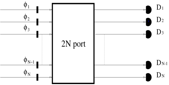
Figure 7.1: The schematic picture of an $2N$ port. There are $N$ phases in front of each input port and $N$ detectors behind each output ports.

An extended introduction to the physics and theory of such devices is given in [Żukowski97b], and therefore the reader not acknowledged with those concepts is kindly asked to consult this reference. Multiport beam splitters were introduced into the literature on the EPR paradox in [Klyshko88, Zeilinger93, Zeilinger94] in order to extend two qubit Bell-phenomena to observables described as operators in Hilbert spaces of dimension higher than two. In contradistinction to the higher than 1/2 spin generalisations of the Bell-phenomena [Mermin80, Garg82, Mermin82, Ardehali91, Agarwal93, Wódkiewicz94, Wódkiewicz95], this type of experimental devices generalise the ideas of beam-entanglement [Horne85, Żukowski88, Horne89, Rarity90]. Unbiased symmetric multiport beam splitters are performing unitary transformations between ”mutually unbiased” bases in the Hilbert space [Schwinger60, Ivanovic81, Wooters86]. They were tested in several recent experiments [Mattle95, Reck96], and also various aspects of such devices were analysed theoretically [Reck94, Jex95].

We shall use here only multiport beam splitters which have the property that the elements of the unitary transformation which describes their action are given by

$$U_{m,m^{\prime}}^{N}={1\over\sqrt{N}}\gamma_{N}^{(m-1)(m^{\prime}-1)},$$ (7.1)

where $\gamma_{N}=\exp(i{2\pi\over N})$ and the indices $m$, $m^{\prime}$ denote the input and exit ports. Such devices were called in [Żukowski97b] the Bell multiports.

7.3 Quantum mechanical predictions

One assumes that the initial $M$ qu$N$it state that feeds $M$ spatially separated multiports, each of which has $N$ inputs and $N$ outputs, has the following form:

$$|\psi(M)\rangle={1\over\sqrt{N}}\sum_{m=1}^{N}\prod_{l=1}^{M}|m\rangle_{l},$$ (7.2)

where $|m\rangle_{l}$ describes the $l$-th qu$N$it being in the $m$-th beam, which leads to the $m$-th input of the $l$-th multiport. Please note, that only one qu$N$it enters each multiport. However, each of the qu$N$its itself is in a mixed state (with equal weights), which gives it equal probability to enter the local multiport via any of the input ports.

Figure 7.2: The scheme of the experiment with four tritters.

The state (7.2) seems to be the most straightforward generalisation of the GHZ states to the new type of observables. In the original GHZ states the number of their components (i.e., two) is equal to the dimension of the Hilbert space describing the relevant (dichotomic) degrees of freedom of each of the qu$N$its. This property is shared with the EPR-type states proposed in [Żukowski97b] for a two-multiport Bell-type experiment - in this case the number of components equals the number of input ports of each of the multiport beam splitters. We shall not discuss here the possible methods to generate such states. However, we briefly mention that the recently tested entanglement swapping [Żukowski93a, Żukowski95, Pan98] technique could be used for this purpose.

As it was mentioned earlier, in front of every input of each multiport beam splitter one has a tunable phase shifter. The initial state is transformed by the phase shifters into

$$|\psi(M)^{\prime}\rangle={1\over\sqrt{N}}\sum_{m=1}^{N}\prod_{l=1}^{M}\exp(i\phi_{l}^{m})|m\rangle_{l},$$ (7.3)

where $\phi_{l}^{m}$ stands for the setting of the phase shifter in front of the $m$-th port of the $l$-th multiport.

The quantum prediction for probability to register the first photon in the output $k_{1}$ of an $2N$ - port device, the second one in the output $k_{2}$ of the second such device ,…, and the $M$-th one in the output $k_{M}$ of the $M$-th device is given by:

$$P_{QM}(k_{1},\dots,k_{M}|\vec{\phi_{1}},\dots,\vec{\phi_{M}})=$$

$$({1\over N})^{M+1}|\sum_{m=1}^{N}\exp(i\sum_{l=1}^{M}\phi_{l}^{m})\prod_{n=1}^{M}\gamma_{N}^{(m-1)(k_{n}-1)}|^{2}=$$

$$=({1\over N})^{M+1}\left[N+2\sum_{m>m^{\prime}}^{N}\cos\left(\sum_{l=1}^{M}\Delta\Phi_{l,k_{l}}^{m,m^{\prime}}\right)\right],$$ (7.4)

where $\Delta\Phi_{l,k_{l}}^{m,m^{\prime}}=\phi_{l}^{m}-\phi_{l}^{m^{\prime}}+{2\pi\over N}(k_{l}-1)(m-m^{\prime})$. The shorthand symbol $\vec{\phi}_{k}$ stands for the full set of phase settings in front of the $k$-th multiport, i.e. $\phi_{k}^{1},\phi_{k}^{2},\dots,\phi_{k}^{N}$.

7.3.1 Bell number assignment

To efficiently describe the local detection events let us employ a specific value assignment method (called Bell number assignment; for a detailed explanation see again [Żukowski97b]), which ascribes to the detection event behind the $m$ - th output of a multiport the value $\gamma_{N}^{m-1}$, where $\gamma_{N}=\exp(i{2\pi\over N})$. With such a value assignment to the detection events, the Bell-type correlation function, which is the average of the product of the expected results, is defined as

$$E(\vec{\phi_{1}},\cdots,\vec{\phi_{M}})=$$

$$=\sum_{k_{1},\cdots,k_{M}=1}^{N}\prod_{l=1}^{M}\gamma_{N}^{k_{l}-1}P(k_{1},\cdots,k_{M}|\vec{\phi_{1}},\cdots,\vec{\phi_{M}})$$ (7.5)

and as we shall see for the quantum case it acquires particularly simple and universal form.

The easiest way to compute the correlation function for the quantum prediction employs the mid formula of (7.4):

$$E_{QM}(\vec{\phi_{1}},\cdots,\vec{\phi_{M}})=$$

$$=({1\over N})^{M+1}\sum_{k_{1},\cdots,k_{M}=1}^{N}\sum_{m,m^{\prime}=1}^{N}\exp\left(i\sum_{n=1}^{M}(\phi_{n}^{m}-\phi_{n}^{m^{\prime}})\right)$$

$$\times\prod_{l=1}^{M}\gamma_{N}^{(k_{l}-1)(m-m^{\prime}+1)}=$$

$$=({1\over N})^{M+1}\sum_{m,m^{\prime}=1}^{N}\exp\left(i\sum_{n=1}^{N}(\phi_{n}^{m}-\phi_{n}^{m^{\prime}})\right)$$

$$\times\prod_{l=1}^{M}\sum_{k_{l}=1}^{N}\gamma_{N}^{(k_{l}-1)(m-m^{\prime}+1)}.$$ (7.6)

Now, one notices that $\sum_{k_{l}=1}^{N}\gamma_{N}^{(k_{l}-1)(m-m^{\prime}+1)}$ differs from zero (and equals to N) only if $m-m^{\prime}+1=0$, modulo N. Therefore we can finally write:

$$E_{QM}(\vec{\phi_{1}},\cdots,\vec{\phi_{M}})$$

$$={1\over N}\sum_{m=1}^{N}\exp(i\sum_{l=1}^{M}\phi^{m,m+1}_{l}),$$ (7.7)

where $\phi^{m,m+1}_{l}=\phi^{m}_{l}-\phi^{m+1}_{l}$ and the above sum is understood modulo N, which means that $\phi^{N+1}_{l}=\phi^{1}_{l}$.

One can notice here a striking simplicity and symmetry of this quantum correlation function (7.7). It is valid for all possible values of M (number of qu$N$its) and for all possible values of $N\geq 2$ (number of ports). For $N=2$, it reduces itself to the usual two qubit, and for $N=2$, $M\geq 2$ the standard GHZ type multi-qubit correlation function for beam-entanglement experiments, namely $\cos(\sum_{l=1}^{M}\phi_{l}^{1,2})$ [Mermin90b]. The Bell - EPR phenomena discussed in [Żukowski97b] are described by (7.7) for $M=2,N\geq 3$.

Even for $N=2$, $M=1$ the function (7.7) describes the following process. Assume that a traditional four-port 50-50 beam splitter, is fed a single photon input in a state in which is an equal superposition of being in each of the two input ports. The value of (7.7) is the average of expected photo counts behind the exit ports (provided the click at one of the detectors is described as $+1$ and at the other one as $-1$), and of course it depends on the relative phase shifts in front of the beam splitter. In other words, this situation describes a Mach-Zehnder interferometer with a single photon input at a chosen input port. For $N=3$, $M=1$ the same interpretation applies to the case of a generalised three input, three output Mach-Zehnder interferometer described in [Weihs96], provided one ascribes to firings of the three detectors respectively $\gamma_{3}=\alpha\equiv\exp(i{2\pi\over 3})$, $\alpha^{2}$ and $\alpha^{3}$.

7.3.2 Perfect correlations

The described set of gedanken experiments is rich in EPR-GHZ correlations (for $M\geq 2$). To reveal the above, let us first analyse the conditions (i.e. settings) for such correlations. As the correlation function (7.7) is an average of complex numbers of unit modulus, one has $|E_{QM}(\vec{\phi_{1}},\cdots,\vec{\phi_{M})}|\leq 1$. The equality signals a perfect EPR-GHZ correlation. It is easy to notice that this may happen only if

$$\exp(i\sum_{l=1}^{M}\phi_{l}^{1,2})=\exp(i\sum_{l=1}^{M}\phi_{l}^{2,3})=\cdots=\exp(i\sum_{l=1}^{M}\phi_{l}^{M,1})=\gamma_{N}^{k},$$

where k is an arbitrary natural number. Under this condition $E(\vec{\phi_{1}},\cdots,\vec{\phi_{M}})=\gamma_{N}^{k}$. This means that only those sets of $M$ spatially separated detectors may fire, which are ascribed such Bell numbers which have the property that their product is $\gamma_{N}^{k}$. Knowing, which detectors fired in the set of $M-1$ observation stations, one can predict with certainty which detector would fire at the sole observation station not in the set.

7.4 Paradoxes for $N+1$ maximally entangled qu$N$its

7.4.1 Four tritters

We shall now present the simplest GHZ-type paradox for such systems. We take $N=3$ and $M=4$. That is we consider now, the experimental situation in which one has the source producing the ensemble of four three-state particles (qutrits) described by the state $|\psi(4)\rangle$ (compare, (7.2)) that feeds four three-port beam splitters (i.e., tritters [Żukowski97b]). In this case the quantum correlation function has the form:

$$E_{QM}(\vec{\phi_{1}},\vec{\phi_{2}},\vec{\phi_{3}},\vec{\phi_{4}})$$

$$={1\over 3}\sum_{k=1}^{3}\exp\left(i\sum_{l=1}^{4}(\phi_{l}^{k}-\phi_{l}^{k+1})\right).$$ (7.8)

The (deterministic) local hidden variables correlation function for this type of experiment must have the following structure [Bell64]:

$$E_{HV}(\vec{\phi_{1}},\vec{\phi_{2}},\vec{\phi_{3}},\vec{\phi_{4}})=\int_{\Lambda}\prod_{k=1}^{4}I_{k}(\vec{\phi_{k}},\lambda)\rho(\lambda)d\lambda.$$ (7.9)

The hidden variable function $I_{k}(\vec{\phi_{k}},\lambda)$, which determines the firing of the detectors behind the k-th multiport, depends only upon the local set of phases, and takes one of the three possible values $\alpha$, $\alpha^{2}$, $\alpha^{3}=1$ (these values indicate which of the detectors is to fire), and $\rho(\lambda)$ is the distribution of hidden variables.

Consider four gedanken experiments. In the first one our observers, each of whom operates one of the spatial separated devices, choose the following phases in front of their three-port beam splitters:

$$\vec{\phi_{1}}\equiv(\phi_{1}^{1},\phi_{1}^{2},\phi_{1}^{3})=(0,{2\pi\over 9},{4\pi\over 9})=\vec{\phi_{2}}=\vec{\phi_{3}}=\vec{\phi}$$

$$\vec{\phi_{4}}\equiv(\phi_{4}^{1},\phi_{4}^{2},\phi_{4}^{3})=(0,0,0)=\vec{\phi^{\prime}}.$$ (7.10)

In the second experiment, the third observer sets $\vec{\phi_{3}}=\vec{\phi^{\prime}}$ whereas the other ones set $\vec{\phi}$. We repeat this swapping of the settings procedure in the next two experiments until the first observer sets $\vec{\phi^{\prime}}$ and the other set $\vec{\phi}$. Quantum mechanics predicts that in all four such experiments the correlation function is equal to $\alpha^{2}$ (i.e. we have perfect GHZ correlations). Namely we have

$$E_{QM}(\vec{\phi},\vec{\phi},\vec{\phi},\vec{\phi}^{\prime})=E_{QM}(\vec{\phi},\vec{\phi},\vec{\phi}^{\prime},\vec{\phi})$$

$$=E_{QM}(\vec{\phi},\vec{\phi}^{\prime},\vec{\phi},\vec{\phi})=E_{QM}(\vec{\phi}^{\prime},\vec{\phi},\vec{\phi},\vec{\phi})=\alpha^{2}.$$ (7.11)

However, this immediately implies that for any local hidden variables theory that aims at describing these phenomena one must have for every $\lambda$

$$I_{k}(\vec{\phi^{\prime}},\lambda)\prod_{{l=1},{l\neq k}}^{4}I_{l}(\vec{\phi},\lambda)=\alpha^{2},$$ (7.12)

and this must hold for all $k=1,2,3,4$. But, since $I_{l}(\vec{\phi},\lambda)^{3}=\alpha^{3k}=1$ (where, $k$ represents a certain integer), then after multiplying these four equations side by side, one has for every $\lambda$

$$\prod_{l=1}^{4}I_{l}(\vec{\phi^{\prime}},\lambda)=\alpha^{2}.$$ (7.13)

Therefore, if the local hidden variable theory is to agree with the earlier mentioned quantum predictions (7.11), then one must have

$$E(\vec{\phi^{\prime}},\vec{\phi^{\prime}},\vec{\phi^{\prime}},\vec{\phi^{\prime}})=\alpha^{2}=\alpha^{*}.$$ (7.14)

However, the quantum prediction is $E_{QM}(\vec{\phi^{\prime}},\vec{\phi^{\prime}},\vec{\phi^{\prime}},\vec{\phi^{\prime}})=1$. Thus we have a GHZ-type contradiction that $1=\alpha^{*}$. I.e., hidden variables predict a different type perfect EPR-GHZ correlation. I.e. we have a realisation of the GHZ paradox for non-dichotomic observables.

7.4.2 General case: $N+1$ maximally entangled qu$N$its

We will extend the reasoning to the case when one has $M=N+1$ qu$N$its (described by the state of the form (7.2)) beamed into multiport beam splitters with $N$ input and output ports. The quantum prediction for the Bell correlation function is given by (7.7), with the appropriate value of $M$.

The local hidden variables correlation function must have the following structure

$$\int\prod_{k=1}^{M}I_{k}(\vec{\psi_{k}},\lambda)\rho(\lambda)d\lambda,$$ (7.15)

where $k$ now extends from $1$ to $M$ and $\vec{\psi_{k}}$ stands for the full set of settings in front of the $k$-th multiport, i.e. $\psi_{k}^{1},\psi_{k}^{2},\cdots,\psi_{k}^{M-1}$, and $I_{k}(\vec{\psi_{k}},\lambda)$ is a hidden variable function depending on the local phase settings, which has the property that its value, which can be any integer power of $\gamma_{M-1}$, indicated which local detector is to fire.

Now, as it was in the previous case, we must choose appropriate phases for each of observers that will be taken in the first experiment. The appropriate choice is the following one:

$$\vec{\psi}_{1}=\cdots=\vec{\psi}_{M-1}=(0,\delta,2\delta,\cdots,(M-2)\delta)=\vec{\psi}$$

$$\vec{\psi}_{M}=(0,\cdots,0)=\vec{\psi^{\prime}},$$ (7.16)

where $\delta={2\pi\over(M-1)^{2}}$. In the next $M-1$ experiments one applies previously described swapping of the settings procedure until the first observer sets $\vec{\psi^{\prime}}$ and the other ones set $\vec{\psi}$. For such choice of phases the quantum correlation function for every of the $M$ experiment, is equal to $\gamma_{M-1}^{M-2}=\gamma_{M-1}^{*}$. (i.e. we have perfect GHZ correlations of the same type for each of the experiments). But this implies that, for any local hidden variables theory that aims at describing these phenomena one must have, for every $\lambda$,

$$I_{k}(\vec{\psi^{\prime}},\lambda)\prod_{l\neq k}I_{l}(\vec{\psi},\lambda)=\gamma_{M-1}^{*},$$ (7.17)

and that this must hold for all $k=1,\cdots,M$. However, after multiplying these $M$ equations one has:

$$\prod_{l=1}^{M}I_{l}(\vec{\psi^{\prime}},\lambda)=\gamma_{M-1}^{*},$$ (7.18)

where we have used the property of the Bell numbers generated by $\gamma_{M-1}$, that each of them to the $M-1$-th power gives 1, and therefore that $I_{k}(\vec{\psi},\lambda)^{M}=1$. Thus, the local hidden variable implies that

$$E_{QM}(\vec{\psi^{\prime}},\cdots,\vec{\psi^{\prime}})=\gamma_{M-1}^{*}.$$

However, the quantum prediction is 1. Thus we have the GHZ contradiction that $1=\gamma_{M-1}^{*}$. I.e. hidden variables predict a different type perfect EPR - GHZ correlations. In other words the EPR idea of elements of reality makes no sense for the discussed experiments, and this hold for an arbitrary number of qu$N$its $M$, and for suitably related ($M-1$), but in principle arbitrarily high number of input and exit ports of symmetric multiport beam splitters.

7.5 Paradoxes for $N$ maximally entangled qu$N$its.

In this section we show that the above reasoning can be as well applied to the case where the number of observers $M$ equals the number of input ports $N$ of the $2N$ port Bell multiports.

7.5.1 Three tritters

As the simplest example let us consider the gedanken experiment with three observers each of which having tritters (3 input and 3 output ports) as a measuring device. The correlation function for such an experiment reads

$$E_{QM}(\vec{\phi}_{1},\vec{\phi}_{2},\vec{\phi}_{3})$$

$$={1\over 3}\sum_{k=1}^{3}\exp\left(i\sum_{l=1}^{3}(\phi_{l}^{k}-\phi^{k+1}_{l})\right).$$ (7.19)

In the first run of the experiment we allow the observers to choose the following settings of the measuring apparatus

$$\vec{\phi}_{1}=(0,{\pi\over 3},{2\pi\over 3})=\vec{\phi}_{2}=\vec{\phi}$$

$$\vec{\phi}_{3}=(0,0,0)=\vec{\phi^{\prime}}$$ (7.20)

in the second run they choose

$$\vec{\phi}_{1}=\vec{\phi^{\prime}}$$

$$\vec{\phi}_{2}=\vec{\phi}=\vec{\phi}_{3}$$

whereas in the third run they fix the local settings of their tritters on

$$\vec{\phi}_{1}=\vec{\phi}=\vec{\phi}_{3}$$

$$\vec{\phi}_{2}=\vec{\phi^{\prime}}.$$ (7.22)

Now, let us calculate the numerical values of the correlation function for each experimental situation. We easily find that for all three experiments this value, due to the special form of the correlation function, is the same and reads

$$E_{QM}(\vec{\phi},\vec{\phi},\vec{\phi^{\prime}})=E_{QM}(\vec{\phi^{\prime}},\vec{\phi},\vec{\phi})=E_{QM}(\vec{\phi},\vec{\phi^{\prime}},\vec{\phi})$$

$$=\exp(-i{2\pi\over 3})=\alpha^{2},$$ (7.23)

i.e., we observe perfect correlations.

Proceeding in exactly the same way as in the previous section we can write the equations that must be fulfilled by local hidden variables for every $\lambda$, i.e.,

$$I_{1}(\vec{\phi},\lambda)I_{2}(\vec{\phi},\lambda)I_{3}(\vec{\phi^{\prime}},\lambda)=\alpha^{2}$$

$$I_{1}(\vec{\phi^{\prime}},\lambda)I_{2}(\vec{\phi},\lambda)I_{3}(\vec{\phi},\lambda)=\alpha^{2}$$

$$I_{1}(\vec{\phi},\lambda)I_{2}(\vec{\phi^{\prime}},\lambda)I_{3}(\vec{\phi},\lambda)=\alpha^{2}$$ (7.24)

After multiplication of the above equations one arrives at:

$$\prod_{k=1}^{3}I_{k}(\vec{\phi^{\prime}},\lambda)\prod_{k=1}^{3}I_{k}(\vec{\phi},\lambda)^{2}=(\alpha^{2})^{3}=1,$$ (7.25)

which can be also written in the following form

$$\prod_{k=1}^{3}I_{k}(\vec{\phi^{\prime}},\lambda)=\prod_{k=1}^{3}I_{k}(\vec{\phi},\lambda),$$ (7.26)

where we have used the property of the hidden variable functions, namely that $I_{k}(\vec{\phi},\lambda)^{2}=I_{k}(\vec{\phi},\lambda)^{*}$ for every $\lambda$. However, because $E_{QM}(\vec{\phi^{\prime}},\vec{\phi^{\prime}},\vec{\phi^{\prime}})=1$ we must also have

$$\prod_{k=1}^{3}I_{k}(\vec{\phi^{\prime}},\lambda)=1,$$ (7.27)

which, because of (7.26), gives

$$\prod_{k=1}^{3}I_{k}(\vec{\phi},\lambda)=1$$ (7.28)

for every $\lambda$. This in turn implies that

$$E_{QM}(\vec{\phi},\vec{\phi},\vec{\phi})=1,$$ (7.29)

which means that local hidden variables predict perfect correlations for the experiment when all observers set their local settings at $\vec{\phi}$. However, the true quantum prediction is that

$$E_{QM}(\vec{\phi},\vec{\phi},\vec{\phi})=-{1\over 3}.$$ (7.30)

Therefore we have the contradiction: $1=-{1\over 3}$.

This contradiction is of the different type than the one derived in the previous section although it has been obtained in the similar way, i.e., the perfect correlations have been used to derive it- equations (7.24) and (7.25). Here local hidden variables imply a certain perfect correlation, which is not predicted by quantum mechanics.

7.5.2 General case: N maximally entangled qu$N$its.

Now, we employ the above procedure for the case when we have an arbitrary odd number of multiports and qu$N$its $N=2m+1$. As we have seen in the previous section the crucial point is to find the proper phases for the multiports. Let us choose for the first gedanken experiment the following ones

$$\vec{\phi}_{1}=(0,{\pi\over 2m+1},{2\pi\over 2m+1},...,{2m\pi\over 2m+1})=\vec{\phi}$$

$$\vec{\phi}_{2}=\vec{\phi}_{3}=...=\vec{\phi}_{2m}=\vec{\phi}$$

$$\vec{\phi}_{2m+1}=(0,0,...,0)=\vec{\phi^{\prime}}.$$ (7.31)

As before, in the next run of the experiment we choose the same phases but we change the role of observers such that in the second run the first one chooses $\vec{\phi^{\prime}}$ while the rest of them choose $\vec{\phi}$, in the third run the third one chooses $\vec{\phi^{\prime}}$ while the rest of them choose $\vec{\phi}$, etc. Again, the value of the correlation function for each experiment is the same

$$E_{QM}(\vec{\phi},...,\vec{\phi^{\prime}})=E_{QM}(\vec{\phi^{\prime}},\dots,\vec{\phi})=\dots=E_{QM}(\vec{\phi},\dots,\vec{\phi^{\prime}},\vec{\phi})$$

$$={1\over 2m+1}\left[\exp\left(-i{2m\pi\over 2m+1}\right)+\exp\left(-i{2m\pi\over 2m+1}\right)\right.$$

$$\left.+...+\exp\left(-i{2m\pi\over 2m+1}\right)+\exp\left(i{4m^{2}\pi\over 2m+1}\right)\right]$$

$$={1\over 2m+1}\left[2m\exp\left(-i{2m\pi\over 2m+1}\right)+\exp\left(i{4m^{2}\pi\over 2m+1}\right)\right]=\gamma_{N}^{-m}$$ (7.32)

Using (7.32), the structure of the hidden variables correlation function (7.15) and multiplying the above equations by each other we arrive at

$$\prod_{k=1}^{2m+1}I_{k}(\vec{\phi^{\prime}},\lambda)=\prod_{k=1}^{2m+1}I_{k}(\vec{\phi},\lambda)^{-2m}=\prod_{k=1}^{2m+1}I_{k}(\vec{\phi},\lambda)$$ (7.33)

for every $\lambda$. Because $E_{QM}(\vec{\phi^{\prime}},\dots,\vec{\phi^{\prime}})=1$ one must have

$$\prod_{k=1}^{2m+1}I_{k}(\vec{\phi^{\prime}},\lambda)=1,$$ (7.34)

which gives

$$\prod_{k=1}^{2m+1}I_{k}(\vec{\phi},\lambda)=1$$ (7.35)

for every $\lambda$. Thus, local hidden variables imply the following perfect correlation

$$E_{QM}(\vec{\phi},...,\vec{\phi})=1,$$ (7.36)

which is untrue because quantum mechanics gives

$$E_{QM}(\vec{\phi},...,\vec{\phi})$$

$$={1\over 2m+1}\left[2m\exp\left(-i\frac{2m+1}{2m+1}\pi\right)\right.$$

$$\left.+\exp\left(i\frac{(2m+1)2m}{2m+1}\pi\right)\right]={-2m+1\over 2m+1}.$$ (7.37)

Therefore, for each $m$ one obtains the untrue identity $1=\frac{-2m+1}{2m+1}$, which in the limit of $m\longrightarrow\infty$ becomes $1=-1$.

Now, let us see what happens when one has the even number of qu$N$its and the multiports $N=2m$ ($m\geq 2$). As before we must find appropriate phases. Let us make the following choice:

$$\vec{\phi}_{1}=(0,{\pi\over 2m-1},{2\pi\over 2m-1},...,{(2m-1)\pi\over 2m-1})=\vec{\phi}$$

$$\vec{\phi}_{2}=\vec{\phi}_{3}=...=\vec{\phi}_{N-1}=\vec{\phi}$$

$$\vec{\phi}_{N}=(0,0,...,0)=\vec{\phi^{\prime}}.$$ (7.38)

One easily finds that

$$E_{QM}(\vec{\phi},\dots,\vec{\phi^{\prime}})=E_{QM}(\vec{\phi^{\prime}},\dots,\vec{\phi})=\dots=E_{QM}(\vec{\phi},\dots,\vec{\phi^{\prime}},\vec{\phi})$$

$$={1\over 2m}\left[(2m-1)\exp\left(-i\frac{2m-1}{2m-1}\pi\right)\right.$$

$$\left.+\exp\left(i\frac{(2m-1)^{2}}{2m-1}\pi\right)\right]=-1$$ (7.39)

and

$$E_{QM}(\vec{\phi},..,\vec{\phi})$$

$$={1\over 2m}\left[(2m-1)\exp\left(-i\frac{2m}{2m-1}\pi\right)+\exp\left(i\frac{2m(2m+1)}{2m+1}\pi\right)\right]$$

$$={1\over 2m}\left[(2m-1)\exp\left(-i\frac{2m}{2m-1}\pi\right)+1\right].$$ (7.40)

Applying the same reasoning as above one has

$$1={1\over 2m}\left[(2m-1)\exp\left(-i\frac{2m}{2m-1}\pi\right)+1\right].$$ (7.41)

Again, for each $m>2$ one has a contradiction, which in the limit of $m\longrightarrow\infty$ becomes $1=-1$.

According to the old quantum rules of thumb one approaches the classical limit with the growing quantum numbers. The above results (for both the odd and the even case) once more show the contrary behaviour.

7.6 Conclusions

The derived paradoxes can be divided into two groups. To the first group belong the series of paradoxes where one has more observers than input ports in the unbiased multiport beamsplitters. Within this group the contradiction manifests itself in different perfect correlations predicted by quantum mechanics and local realism. As a special case one obtains the original GHZ paradox.

In the second group one has the series of paradoxes in which the number of observers and input ports in the unbiased multiport beamsplitters is the same. Within this group the derivation of the paradoxes relies on the perfect correlations (as in the first group) but the final result is different. The resulting contradiction between quantum mechanics and local realism manifests itself in the fact that local realism predicts a certain perfect correlation whereas quantum mechanics does not.

An interesting feature of paradoxes within the second group is that they naturally split into two parts: the even and the odd number of observers (input ports). In each part the final contradiction has different numerical values. Furthermore, for the case of two observers one cannot derive the GHZ paradox with the method presented here.

All paradoxes do not vanish with the growing dimension $N$ of the Hilbert space describing each qu$N$it.

In conclusion we state that the multiport beam splitters, and the idea of value assignment based Bell numbers, lead to a strikingly straightforward generalisation of the GHZ paradox for entangled qu$N$its. These properties may possibly find an application in future quantum information and communication schemes (especially as GHZ states are now observable in the lab [Bouwmeester99]).

Part III Extension of Bell Theorem via numerical approach

***

   

In the present part of the dissertation a novel approach to the Bell theorem, via numerical linear optimisation, will be presented. This approach enables one to first of all solve the old question of generalisation of the Bell theorem to

• more possible settings at each side of the experiment (for two and three qubits)

• entangled pairs of qu$N$its ($N>2$) (in earlier literature called spins higher than $\frac{1}{2}$)

The early Bell theorem involved only two entangled qubits and two observers, who could choose among two local mutually incompatible observables. Generalisations involving more than two observers were considered by many authors and here in the previous sections. However, one can ask the following question what the necessary and sufficient conditions for local realistic description of situations in which each observer can choose from more than two observables, and for the case when two observables are not of a dichotomic nature are.

There were several attempts to unite Bell inequalities for such problems, however only the stage of necessary conditions for local realism was reached. No one has been able to construct the full set of Bell inequalities for such problems which would provide the sufficient condition for local realistic description.

This was a serious issue, since necessary conditions are per se weaker than sufficient ones. Several papers were written discussing the exploding algebraic difficulty in finding sufficient sets of Bell inequalities [Peres99]. For example Peres gives as a number of the so called Farkas vectors (effectively coefficients in generalised Clauser-Horne inequalities) for a two qu$N$it experiment with only two observables (non-degenerate) allowed to be measured at each side [Peres99]. It reads $N_{F}(N)=(2^{N}-2)^{4}$, i.e., one has $N_{F}(2)=16,N_{F}(3)=1296$ etc. This causes that the computational time grows extremely fast not allowing one to calculate anything in reasonable time.

However if one asks directly the question whether the probabilities given by quantum mechanics are describable via a local realistic theory, it turns out that this question can be formulated as a typical linear optimisation problem. Since excellent numerical methods exist it turns out that for the number of settings of the order of 10 for two qubits and of the order of 4 for three qubits, and for qu$N$its with $N$ up to 10, such problems are solvable on a standard work-station with the computing time of the order of one day. The algorithm to tackle these problems together with the results will be presented here.

The threshold noise, or in other words visibility, below which there is no local realistic model for two and three maximally entangled qubits is of the same value as in the case of standard Bell inequalities (involving only two settings at each side). Nevertheless, the presented approach gives a new method of a direct analysis of experimental data. Such data can be directly tested for a possibility of a local realistic model of them (without any of the usual hypothesis about the curves best fitting to the data).

In the case of the second problem, entangled qu$N$its, new surprising results have been obtained. The computer data reveal growing discrepancy of the quantum predictions with local realism with the increasing dimensionality of the Hilbert space of the sub-systems. Earlier approaches suggested contrary behaviour (see , for instance, [Mermin80, Mermin82]).

Chapter 8 Necessary and sufficient conditions to violate local realism for two maximally entangled qubits- extension to more than two local settings [7]

8.1 Introduction

It is a common wisdom in the quantum optical community that the threshold visibility of the sinusoidal two-qubit interference pattern beyond which the Bell inequalities are violated is (for the case of perfect detectors) $\frac{1}{\sqrt{2}}$ (see, e. g. [Clauser78]). Most of the experiments exceed that limit (with the usual “fair sampling assumption”) [Freedman72, Ou88, Rarity90, Kwiat93, Pittman95, Tittel98]. Some difficulties to reach this threshold were observed in the very early experiments [Clauser78], as well as in some recent ones involving novel techniques. Thus far, in atomic interferometry EPR experiments [Hagley97] and for the phenomenon of entanglement swapping [Żukowski95, Pan98], the resulting visibility is less than the magic $71\%$.

It is also well known that the Clauser-Horne inequality and the CHSH inequality are not only necessary conditions for the existence of local realistic models but also sufficient [Fine82] (in the case of the CHSH inequality, this requires some simplifying assumptions [Garg87]). However, the sufficiency proofs used involve only two pairs of settings of the local macroscopic parameters (e.g. orientations of the polarisers) that define the measured local observables. Thus, the constructions are valid for precisely those settings and nothing more, and there is no guarantee that the models can be extended to more settings. Consequently one may ask what is the maximal visibility for a model applicable to all possible settings of the measuring apparata, that returns sinusoidal two qubit interference fringes. It is already known that for perfect detectors, this value cannot be higher than $\frac{1}{\sqrt{2}}$ or lower than $2/\pi$ (this is the visibility of the recent ad hoc model by Larsson [Larsson99]; for earlier models returning visibilities of $50\%$ see e.g. [Wódkiewicz91]).

The knowledge of the maximal visibility of sinusoidal two-qubit fringes in a Bell-type experiment that still can be fully modelled in a local realistic way, may help us to distinguish better between ‘local’ and ‘nonlocal’ density matrices. For two two-state systems one can find precise conditions which have to be satisfied by density matrices describing the general state, pure or mixed, of the full system, that enable violation of the CHSH inequalities [Horodecki95]. States fulfilling such conditions are often called “nonlocal”. However, since the CHSH inequality is necessary and sufficient only for two pairs of settings, it is not excluded a priori that some states that satisfy such inequalities for all possible sets of two pairs of local dichotomic observables, nevertheless give predictions that in their entirety cannot be modelled by local hidden variables. Such models must first of all reproduce the full continuous sinusoidal variation of two-qubit interference fringes, as well as the other predictions.

It is clear that the full solution of the question would require a construction, or a proof of existence, of local hidden variable models which return sinusoidal fringes of the maximal possible visibility, that are applicable for all possible settings of the measuring apparata. Since this seems to be very difficult, we chose a numerical method of point wise approximation at a finite number of settings at each side of the experiment. Due to exponential growth of the computation time when the number of settings increases, we managed to reach up to 10 settings on each side, i.e. up to 100 measurements points (which due to a certain symmetry, about which we will say more later, effectively can be transformed into $20\times 20=400$ points). The exponential growth hinders any substantial increase in this number. Such numerical models cannot give a definite answer concerning the critical visibility of sinusoidal fringes, however our calculations enable us to put forward a strong conjecture that this value must be indeed ${1\over\sqrt{2}}$ (see below). The numerical method presented in this chapter is applied to the correlation function for two qubits. The alternative approach, much better suited for general problems is to apply the method to probabilities of all events that are observed in the experiment. However, for maximally entangled two qubit state, with the interference visibility reduced by some noise (the generic problem studied here) application of numerical approach to correlation function is equivalent to a similar procedure with probabilities, and what is important due to the fact that it leads to a less complicated linear optimisation problem it allows to have numerical results for much more settings on each side than the method involving probabilities. Nevertheless the algorithm involving probabilities was also written, and it returns identical results. It will be presented in the chapter on two entangled qu$N$it problem.

Experimentally our problem can be formulated in the following way: the two qubit state produced by the source does not allow for single qubit interference, and in the experiment less-than-perfect two-qubit fringes are obtained, due to some fundamental limitations (like those present in the case of entanglement swapping, e.g. [Żukowski95, Pan98]) or due to imperfections of the devices. What is the critical two qubit interference visibility beyond which the observed process falsifies local realism? We shall ask these questions assuming, for simplicity, perfect detection efficiencies, which is possible theoretically, and experimentally thus far amounts to the usual “fair sampling assumption”.

Furthermore, the problem may be investigated without the use of the assumption that the observed fringes are of a sinusoidal nature even though the observed two-qubit fringes in experiments with high photon counts follow almost exactly the sinusoidal curves [Freedman72, Ou88, Rarity90, Kwiat93, Pittman95, Tittel98]. In experiments with lower count rates, still with relatively good level of confidence the recorded data have approximately the same character, and it is customary to fit them with sinusoidal curves. It is now a standard procedure to perform the two-qubit interference experiments by recording many points of the interference pattern, rather than stabilising the devices at measurement settings appropriate for the best violation of some Bell inequality. Further, in some of the experiments, e.g. those involving optical fibre interferometers it was not possible to stabilise the phase differences and what is observed is just the interference pattern changing in time, and the visibility of the sinusoidal two-qubit fringes is used as the critical parameter [Tapster94].

Even though the numerical calculations presented here only reach $20\times 20$ points, this is more than enough in comparison to the experimental data. The usual experimental scans rarely involve more than 20 points. Further, our algorithm can be applied directly to the measurement data, and in that way one can even avoid the standby hypothesis that the fringes follow a sinusoidal pattern. The algorithm can directly answer the question: are the data compatible with local realism or not? Since physics is an experimental science, the questions about Nature get their final answers solely in this way.

8.2 Quantum mechanical and local realistic description of the gedanken experiment

We consider the following gedanken experiment. Two observers $a$ and $b$ perform measurements of observables $\vec{a}\cdot\vec{\sigma}$ (observer $a$) and $\vec{b}\cdot\vec{\sigma}$ (observer $b$) on the state defined by the equation (2.1). Observer $a$ can choose between $N_{a}$ settings of the measuring apparatus, which are defined by vectors $\vec{a}_{i}$ ($i=1,\dots,N_{a}$) whereas observer $b$ can choose between $N_{b}$ settings of the measuring apparatus defined by vectors $\vec{b}_{j}$ ($j=1,\dots,N_{b}$). Therefore, they perform $N_{a}\times N_{b}$ mutually exclusive experiments. For each experiment one has the following quantum probabilities (see the equation (6.1))

$$P_{QM}^{V_{2}}(l,m|\vec{a}_{i},\vec{b}_{j})={1\over 4}(1-lmV_{2}\vec{a}_{i}\cdot\vec{b}_{j})$$ (8.1)

and the quantum correlation function

$$E_{QM}^{V_{2}}(\vec{a}_{i},\vec{b}_{j})=-V_{2}\vec{a}_{i}\cdot\vec{b}_{j}.$$ (8.2)

There is no one qubit interference, i.e., $P_{QM}^{V_{2}}(l|\vec{a}_{i})=P_{QM}^{V_{2}}(m|\vec{b}_{j})={1\over 2}$ for all $i,j$.

If one assumes that the unit vectors which define the measured observables are always coplanar the correlation function can be simplified to $E^{V_{2}}_{QM}(\alpha_{i},\beta_{j})=-V_{2}\cos{(\alpha_{i}+\beta_{j})}$ (with the obvious definition of $\alpha_{i}$ and $\beta_{j}$).

Please note that in the considered here gedanken experiment there is one-to-one equivalence between the quantum correlation function and quantum probabilities (see (8.1) and (8.2)). Therefore, we can use either the quantum correlation function or the quantum probabilities to describe the experiment. However, the description of the experiment in terms of the quantum correlation function is more convenient from the numerical point of view, which we will be seen further.

From the numerical values of the quantum correlation function we form a certain matrix $\hat{Q}_{V_{2}}$ of quantum predictions with the entries: $Q_{ij}(V_{2})=E^{V_{2}}_{QM}(\vec{a}_{i},\vec{b}_{j})$.

Within the local hidden variables formalism the correlation function must have the following structure

$$E_{LHV}(\vec{a}_{i},\vec{b}_{j})=\int d\lambda\rho(\lambda)A(\vec{a}_{i},\lambda)B(\vec{b}_{j},\lambda),$$ (8.3)

where for dichotomic measurements

$$A(\vec{a}_{i},\lambda)=\pm 1$$ (8.4)

and

$$B(\vec{b}_{j},\lambda)=\pm 1,$$ (8.5)

and they represent the values of local measurements predetermined by the local hidden variables, denoted by $\lambda$, for the specified local settings. This expression is an average over a certain local hidden variables distribution $\rho(\lambda)$ of certain factorisable matrices, namely those with elements given by $M_{ij}(\lambda)=A(\vec{a}_{i},\lambda)B(\vec{b}_{j},\lambda)$. The symbol $\lambda$ may hide very many parameters. However, since the only possible values of $A(\vec{a}_{i},\lambda)$ and $B(\vec{b}_{j},\lambda)$ are $\pm 1$ there are only $2^{N_{a}}$ different sequences of the values of $(A(\vec{a}_{1},\lambda),A(\vec{a}_{2},\lambda),...,A(\vec{a}_{N_{a}},\lambda))$, and only $2^{N_{b}}$ different sequences of $(B(\vec{b}_{1},\lambda),B(\vec{b}_{2},\lambda),...,B(\vec{b}_{N_{b}},\lambda))$ and consequently they form only $2^{N_{a}+N_{b}}$ matrices $\hat{M}(\lambda)$.

Therefore the structure of local hidden variables models of $E_{LHV}(\vec{a}_{i},\vec{b}_{j})$ reduces to discrete probabilistic models involving the average of all the $2^{N_{a}+N_{b}}$ matrices $\hat{M}(\lambda)$. In other words, the local hidden variables can be replaced, without any loss of generality, by a certain pair of variables $k$ and $l$ that have integer values respectively from $1$ to $2^{N_{a}}$ and from $1$ to $2^{N_{b}}$. To each $k$ we ascribe one possible sequence of the possible values of $A(\vec{a}_{i},\lambda)$, denoted from now on by $A(\vec{a}_{i},k)$, similarly we replace $B(\vec{b}_{j},\lambda)$ by $B(\vec{b}_{j},l)$. With this notation the possible local hidden variables models of the correlation function $E_{LHV}(\vec{a}_{i},\vec{b}_{j})$ acquire the following simple form

$$E_{LHV}(\vec{a}_{i},\vec{b}_{j})=\sum_{k=1}^{2^{N_{a}}}\sum_{l=1}^{2^{N_{b}}}p_{kl}A(\vec{a}_{i},k)B(\vec{b}_{j},l),$$ (8.6)

with, of course, the probabilities satisfying $p_{kl}\geq 0$ and $\sum_{k=1}^{2^{N_{a}}}\sum_{l=1}^{2^{N_{b}}}p_{kl}=1$.

The special case that we study here enables us to simplify the description further. To satisfy the additional requirement that the local hidden variables model returns the quantum prediction of equal probability of the results at the local observation stations, that $P_{QM}^{V_{2}}(l|\vec{a})=P_{QM}^{V_{2}}(m|\vec{b})={1\over 2}$, one can use the following observation. For each $k$, there must exist a $k^{\prime}\neq k$ with the property that $A(\vec{a}_{i},k^{\prime})=-A(\vec{a}_{i},k)$, and similarly for each $l$, there must exist an $l^{\prime}\neq l$ for which $B(\vec{b}_{j},l^{\prime})=-B(\vec{b}_{j},l)$. Then $A(\vec{a}_{i},k)B(\vec{b}_{j},l)=A(\vec{a}_{i},k^{\prime})B(\vec{b}_{j},l^{\prime})$, and thus they give exactly the same matrix of local hidden variables predictions. By assuming $p_{kl}=p_{k^{\prime}l^{\prime}}$ the property of total randomness of local results will always be reproduced by the local hidden variables models, and the generality will not be reduced since the contributions of $p_{kl}$ and $p_{k^{\prime}l^{\prime}}$ to (8.6) cannot be distinguished. Hence, we will always take only one representative of the two pairs, reducing in this way the number of probabilities and matrices of LHV predictions in (8.6) by a factor of two. This is equivalent to taking only half of different $B(\vec{b}_{j},l)$ (or $A(\vec{a}_{i},k)$ for the situation is symmetrical), say, first $2^{N_{b}-1}$ ones. Thus, (8.6) acquires the form

$$E_{LHV}(\vec{a}_{i},\vec{b}_{j})=\sum_{k=1}^{2^{N_{a}}}\sum_{l=1}^{2^{N_{b}-1}}\tilde{p}_{kl}A(\vec{a}_{i},k)B(\vec{b}_{j},l),$$ (8.7)

where we still assume that $\sum_{k=1}^{2^{N_{a}}}\sum_{l=1}^{2^{N_{b}-1}}\tilde{p}_{kl}=1$.

Another reduction by a factor of four is given by the fact that in the coplanar case, the choice of the settings may be limited on each side to ranges not greater than $\pi$ (i.e. $\phi\leq\alpha_{i}\leq\phi+\pi,\psi\leq\beta_{j}\leq\psi+\pi$). This is due to the simple observation that a model of the type (8.6) once established for such settings can be easily extended to settings $\alpha_{i}^{{}^{\prime}}=\alpha_{j}+\pi,\beta_{j}^{{}^{\prime}}=\beta_{j}+\pi$ by putting $A(\alpha_{i}^{{}^{\prime}},l)=-A(\alpha_{i},l)$ and $B(\beta_{j}^{{}^{\prime}},l)=-B(\beta_{j},l)$.

The conditions for local hidden variables to reproduce the quantum prediction with a final visibility $V_{2}$ can be simplified to the problem of maximising a parameter $V_{2}$ for which exists a set of $2^{N_{a}+N_{b}-1}$ probabilities $\tilde{p}_{kl}$, such that

$$\sum_{k=1}^{2^{N_{a}}}\sum_{l=1}^{2^{N_{b}-1}}\tilde{p}_{kl}A(\vec{a}_{i},k)B(\vec{b}_{j},l)=Q_{ij}(V_{2}).$$ (8.8)

Because, for the given local settings (8.8) imposes linear constraints on the probabilities and the visibility, and we are looking for the maximal $V_{2}$, the problem can be solved by means of linear programming- a certain method of optimisation.

8.3 Linear programming and Downhill Simplex Method

Let us briefly describe the idea of linear programming sending more interested readers to the excellent book by Gass [Gass75].

The set of linear equations (8.8) constitute a certain region in a $D=2^{N_{a}+N_{b}-1}+1$ dimensional real space- $2^{N_{a}+N_{b}-1}$ probabilities plus the visibility. The border of the region consists of hyper planes each defined by one of the equations belonging to (8.8); thus, if the equations do not contradict each other the region is a convex set with a certain number of vertices. On this convex set we define a linear function (cost function) $f(p_{1},\cdots,p_{2^{N_{a}+N_{b}-1}},V_{2})=V_{2}$, which maximum we seek.

The fundamental theorem of linear programming states that the cost function reaches its maximum at one of the vertices. Hence, it suffices to find numerical values of the cost function calculated at the vertices and then pick up the largest one. Of course, the algorithmic implementation of this simple idea is not so easy for we must have a method of finding the vertices for which the value of the function continually increases so that the program reaches the optimal solution in the least possible number of steps. Calculating the value of the cost function at every vertex would take too much time as there may be too many of them.

There are lots of excellent algorithms which solve the above optimisation problem. Here we have used the algorithm invented by Gondzio [Gondzio95] and implemented in the commercial code HOPDM 2.30 (Higher Order Primal-Dual Method) written in C programming language.

However, finding the maximal visibility for the given local settings of the measuring apparata is not enough. We should remember that our main goal is to find such local setting for which the threshold visibility is the lowest one. The maximal visibility $V^{max}_{2}$ returned by the HOPDM 2.30 procedure depends on the local settings entering right hand side of (8.8). Thus, returned $V^{max}_{2}$ can be treated as the many variable function, which depends on $N_{a}+N_{b}$ angles in the coplanar case and two times more in the non coplanar one, i.e., $V_{2}^{max}=V_{2}^{max}(\vec{a}_{1},\dots,\vec{a}_{N_{a}},\vec{b}_{1},\dots,\vec{b}_{N_{b}})$.

Hence, we should also have a numerical procedure which finds the minimum of $V^{max}_{2}$. Because we do not know much about the structure of $V^{max}_{2}$ as a function of the local settings the only reasonable method of finding the $V^{max}_{2}$ minimum is the Downhill Simplex Method (DSM) [Nelder65]. The way it looks for the extremum is the following. If the dimension of the domain of a function is $Dim$ the DSM randomly generates $Dim+1$ points. This way it creates a starting simplex, which vertices are these points. Then it calculates the value of a function at the vertices and starts exploring the space by stretching and contracting the simplex. In every step when it finds a vertex where the value of the function is lower then in others it ”goes” in this direction. For more elaborate discussion of this issue see [Nelder65].

8.3.1 Numerical difficulties

Obviously there are some numerical limitations of our computer program. First of all it is obvious that the time needed for computation grows with the number of local settings $N_{a},N_{b}$. For the given $N_{a},N_{b}$ we have $2^{N_{a}+N_{b}-1}+1$ unknowns and $N_{a}\times N_{b}+2$ linear constraints imposed on them. Furthermore, the dimension of the domain of $V^{max}_{2}$ is in general $2N_{a}+2N_{b}$, which makes it harder for the DSM procedure to find a global minimum of $V^{max}_{2}$.

Secondly, the amount of the memory needed to store ”hidden” matrices grows exponentially with $N_{a}$ and $N_{b}$. All these problems taken together has limited our research to the cases where $N_{a}+N_{b}\leq 20$.

It is worth mentioning at this point about the advantages of using the quantum correlation function instead of quantum probabilities as the description of the gedanken experiment. If we are to use probabilities we will have $2^{N_{a}+N_{b}}+1$ unknowns ($2^{N_{a}+N_{b}}$ probabilities plus the visibility $V_{2}$) and $4\times N_{a}\times N_{b}+1$ constraints. Because we struggle with the memory capacity and the computation time every reduction in the number of unknowns and constraints is a great advantage.

Recently A. Peres [Peres99] has discussed the algorithms which search for so-called Farkas vectors, which in turn define coefficients in generalised Bell-inequalities, the set of which is a sufficient and necessary condition for classical probabilistic model (here, essentially, local realistic) to reproduce a certain set of probabilities for pairs of experiments. However, his method explodes numerically much much faster then ours. Simply, our method is applied directly to a certain finite set of specified quantum probabilities. Whereas inequalities based on the Farkas lemma apply to all possible sets of probabilities.

8.4 Results

First of all, we have performed calculations in the coplanar case. We have checked situations in which the number of settings for observer $a$ and $b$ is the same, i.e., $N_{a}=N_{b}=2,3,4,\dots,10$ as well as the cases in which the number of settings for observer $a$ and $b$ is different, i.e., $N_{a}\neq N_{b}$. Because of mentioned limitations of the computer program we could only reach the limit of $N_{a}+N_{b}=20$ in both cases, i.e., for the equal and unequal number of the settings at each side.

Because of the richness of $N_{a}+N_{b}$ dimensional space (coplanar case) to find a global minimum of $V^{max}_{2}$ for the cases where $N_{a}+N_{b}\leq 12$ we have run the DSM procedure $30$ times with varied starting points. For the higher dimensional ones, i.e., where $13\leq N_{a}+N_{b}\leq 15$ we have run the DSM only a few times whereas for the extremal cases, i.e., where $16\leq N_{a}+N_{b}\leq 20$ we have not used the DSM but we simply have calculated $V^{max}_{2}$ on some sets of angles containing (or not) the Bell angles (the definition of the Bell angles is given below).

For $N_{a}+N_{b}\leq 15$ the DSM has always converged to $V^{max}_{2}={1\over\sqrt{2}}$ within the given numerical precision of computation. Furthermore, within the angles $\alpha_{i},\beta_{j}$ ($i=1\dots N_{a},j=1\dots N_{b}$) for which the optimum has been achieved there has been always the subset of four ones (we call the angles belonging to this subset the Bell angles) for which the maximal violation of the CHSH inequality occurs. In other words it means that in the quantum matrix $\hat{Q}$ (matrix of results for the visibility equal one) with entries calculated for the optimal local settings found by the DSM, i.e., settings for which $V_{2}^{max}$ reaches its minimum, a $2\times 2$ sub matrix $\hat{B}$ appears with moduli of all its elements equal to ${1\over\sqrt{2}}$, and three of them of the same sign, e.g.

$$\hat{B}=\left(\begin{array}[]{cc}-{1\over\sqrt{2}}&-{1\over\sqrt{2}}\\[5.69054pt] -{1\over\sqrt{2}}&+{1\over\sqrt{2}}\end{array}\right).$$ (8.11)

Of course, the elements of $\hat{B}$ can be scattered throughout the matrix $\hat{Q}$ but by relabelling the indices it is always possible, for instance, to have $\hat{B}$ in the left hand corner of $\hat{Q}$.

For the combinations of the number of local settings at each side of the gedanken experiment such that $16\leq N_{a}+N_{b}\leq 20$ we have calculated $V^{max}_{2}$ on the sets of local settings including the Bell angles with exactly the same result, i.e., $V_{2}^{max}={1\over\sqrt{2}}$ whereas for the sets of the settings not including the Bell angles $V_{2}^{max}>{1\over\sqrt{2}}$.

We have also tested non coplanar settings with exactly the same result. The visibility was higher than ${1\over\sqrt{2}}$ if among the local settings were no the Bell angles (no sub matrix $\hat{B}$) and it was exactly ${1\over\sqrt{2}}$ otherwise (sub matrix $\hat{B}$ present).

8.4.1 Exemplary numerical model

Let us show an example of the computer solution for the $3\times 3$ coplanar case with the optimisation over local settings of the measuring apparata (the DSM has been used). The threshold visibility for the optimal settings found by the program is $V^{max}_{2}=0.707$ whereas the quantum matrix is given below

$$\hat{Q}_{V^{max}_{2}}=V^{max}_{2}\hat{Q}=V^{max}_{2}\left(\begin{array}[]{ccc}0.107&-0.994&-0.399\\ -0.707&-0.707&-0.964\\ -0.707&0.707&-0.266\end{array}\right).$$ (8.15)

The computer hidden variable model reproducing the above matrix reads

$$\tilde{p}(-1-1-1;+1+1+1)=0.250$$

$$\tilde{p}(+1+1-1;+1-1+1)=0.060$$

$$\tilde{p}(+1+1-1;+1-1-1)=0.135$$

$$\tilde{p}(-1-1+1;+1+1+1)=0.157$$

$$\tilde{p}(+1-1+1;+1+1+1)=0.026$$

$$\tilde{p}(+1-1+1;+1+1-1)=0.067$$

$$\tilde{p}(-1+1-1;+1-1-1)=0.055$$

$$\tilde{p}(+1-1-1;+1-1+1)=0.217$$

$$\tilde{p}(+1-1-1;+1-1-1)=0.033,$$ (8.16)

where, for instance, $\tilde{p}(+1+1-1;+1-1+1)$ denotes the probability of appearing the factorisable matrix $\hat{M}$

$$\hat{M}=\left(\begin{array}[]{ccc}+1&-1&+1\\ +1&-1&+1\\ -1&+1&-1\end{array}\right)=\left(\begin{array}[]{c}+1\\ +1\\ -1\end{array}\right)\left(\begin{array}[]{c}+1\\ -1\\ +1\end{array}\right)^{T}$$ (8.26)

($T$ denotes ordinary transposition).

This example clearly exhibits the characteristic trait which has been mentioned already, namely that in the matrix $\hat{Q}$ there is a sub matrix $\hat{B}$ corresponding to the matrix obtained for the Bell angles- here the elements $Q_{21},Q_{31},Q_{32},Q_{22}$.

The numerical precision of the entries of the matrix $\hat{Q}$ and the visibility $V^{max}_{2}$ is in this example $10^{-3}$. Of course the precision can be increased when necessary but this makes the time of computation longer. However, in some cases we have run the program with the numerical precision of order $10^{-6}$ with the same result, i.e., the $V_{2}^{max}=0.707107\pm 10^{-6}$.

8.5 Application to experimental data

To apply our computer program for analysis of experimental data we replace $Q_{ij}(V_{2})$ in (8.8) by the measured values $E^{QM}_{ij}(exp)$, and perform the same task. If the critical $V_{2}$ returned by the program is less than $1$, the data cannot be reproduced by any local hidden variable model. Note that one even does not have to know what the settings are.

In a recent Bell-type experiment Weinfurter and Michler have obtained the following matrix of results

$$\hat{Q}^{exp}=\left(\begin{array}[]{ccc}-0.894&-0.061&0.761\\ -0.851&0.343&0.765\\ -0.625&0.688&0.516\\ -0.251&0.860&0.103\\ 0.226&0.921&-0.389\\ 0.530&0.651&-0.648\\ 0.855&0.323&-0.832\\ 0.852&-0.092&-0.843\\ 0.785&-0.539&-0.638\\ 0.397&-0.795&-0.253\\ \end{array}\right).$$ (8.27)

The program gives the verdict that the values of all entries to the matrix of results have to be reduced by the factor of $0.796$ to be describable by local hidden variables.

Some explanation is needed here. The entries of (8.27) give the values of the correlation function - there were three different setting on side A of the experiment and 27 settings on side B, however only 10 of them are shown here. In the actual experiment only data from a pair of detectors were collected. To obtain the matrix we have used the usual assumption that $E(\alpha,\beta)=4P(+,+;\alpha,\beta)-1.$ We have also renormalised the numbers of photon pairs counted, so that the average of the counts over approximately two periods of settings at side B represents the probability of $\frac{1}{4}$ (in concurrence with the quantum prediction). To this end we have used data for all 27 settings on side B.

In the recent long-distance EPR-Bell experiment the following set of values of the correlation function was obtained:

$$\hat{Q}^{exp}=\left(\begin{array}[]{cc}0.960&-0.102\\ 0.903&-0.375\\ 0.733&-0.660\\ 0.479&-0.809\\ 0.191&-0.903\\ -0.120&-0.923\\ -0.429&-0.807\\ -0.666&-0.656\\ -0.842&-0.395\\ -0.951&-0.152\\ -0.953&0.171\\ \end{array}\right).$$ (8.28)

This matrix has to be reduced by the factor of $0.737$ to have a local realistic description.

8.6 Conclusions

In his paper Peres [Peres99] has conjectured that if the CH inequalities are satisfied for all possible subsets of two settings on one side and two settings on the other (out of all $N_{a}\times N_{b}$ settings) then this is sufficient for a local realistic model for all $N_{a}\times N_{b}$ settings. Our numerical calculations strongly support this conjecture.

Furthermore, for the situations characterised by the condition $N_{a}+N_{b}\leq 12$ we have found the ultimate value of the visibility still admitting the existence of local hidden variables. Surely, we must be aware of the fact that the DSM may have not found a global minimum of $V^{max}_{2}$, in which the case the threshold $V_{2}$ would be lower than ${1\over\sqrt{2}}$. However, we think that this is highly improbable, which is strongly supported by calculations for $N_{a}+N_{b}>12$.

As it has been shown on two examples our computer program can be also used to analyse directly the raw experimental data. Here the analysis in terms of the correlation function has been performed. However, this is not necessary. In the chapter concerning two maximally entangled qu$N$its (including also qubits) we will present a computer program entirely based on the quantum probabilities rather then on the correlation function. This is important because the one-to-one equivalence between the correlation function and probabilities is valid only if one assumes that certain symmetries concerning probabilities are present (see (8.1)). In the real experiment one may expect that these symmetries are not always fulfilled. The program based on probabilities utterly solves this problem allowing us to analyse real experiments basing solely on the observed clicks of detectors.

To conclude, the performed calculations enable us to put forward the following conjecture: sinusoidal two-qubit fringes of visibility up to $\frac{1}{\sqrt{2}}$ are describable by local realistic theories. At this stage we are not able to give an analytic proof of the above. However, for finite sets of measurement points the results of data analysis with the use of our program fully concur with this hypothesis. One can even say that this is more than enough, since one cannot experimentally test exact sinusoidal nature of the two qubit fringes. The real output of an experiment are count rate sequences at finite number of the measurement points which follow sinusoidal-like pattern. To such data our program can be directly applied giving verdict whether the data admit a local realistic model or not.

Chapter 9 Necessary and sufficient conditions to violate local realism for three maximally entangled qubits- extension to more than two local settings

Exactly the same question on the threshold visibility allowing local and realistic description for all positions of measuring apparata can be posed in the case of correlations involving three qubits instead of two ones. Up to now, the threshold visibility for three qubit correlations (GHZ correlations) is known to be $V_{2}(3)={1\over 2}$ (in the brackets we show that we deal with the visibility for three qubits to distinguish it from the visibility for two qubits $V_{2}$.) [Mermin90b]. However, this limit has been established for the case when there are two local settings of the measuring apparatus at each side of the experiment and it has been obtained in a standard way, i.e., as a condition for the violation of an appropriate Bell inequality.

From the previous section we know that there is a more direct method of finding the numerical value of the threshold visibility, which in addition gives necessary and sufficient conditions for the existence of local hidden variables for the given set of local settings for each observer. In this section we show the application of the presented numerical method to the GHZ correlations, i.e., to the maximally entangled state of three qubits. Surprisingly, the obtained results bear great resemblance to those for two qubits.

9.1 Description of the method

To this end let us consider the following maximally entangled state of 3 qubits

$$|\psi\rangle={1\over\sqrt{2}}(|0\rangle_{1}|0\rangle_{2}|0\rangle_{3}+|1\rangle_{1}|1\rangle_{2}|1\rangle_{3})$$ (9.1)

where $|i\rangle_{j}$ is the $i$-th state of the $j$-th qubit.

Each observer measure the observable $\vec{n}\cdot\vec{\sigma}$, where $n=a,b,c$ ($a$ for the first observer, $b$ for the second one and $c$ for the third one), $\vec{n}$ is a unit vector characterising the observable which is measured by observer $n$ and $\vec{\sigma}$ is a vector the components of which are standard Pauli matrices. As in the case of two qubits the family of observables $\vec{n}\cdot\vec{\sigma}$ covers all possible dichotomic observables for a qubit system, endowed with a spectrum consisting of $\pm 1$.

The probability of obtaining the result $m=\pm 1$ for the observer $a$, when measuring the observable characterised by the vector $\vec{a}$, the result $l=\pm 1$ for the observer $b$, when measuring the observable characterised by the vector $\vec{b}$ and the result $k=\pm 1$ for the observer $c$, when measuring the observable characterised by the vector $\vec{c}$ is equal to

$$P_{QM}(m,l,k;\vec{a},\vec{b},\vec{c})={1\over 8}(1+mla_{3}b_{3}+mka_{3}c_{3}+lkb_{3}c_{3}$$

$$+mlk\sum_{r,p,s=1}^{3}M_{rps}a_{r}b_{p}c_{s}),$$ (9.2)

where $a_{r},b_{p},c_{s}$ are components of vectors $\vec{a},\vec{b},\vec{c}$ and where nonzero elements of the tensor $M_{rps}$ are $M_{111}=1,M_{122}=-1,M_{212}=-1,M_{221}=-1$. In spherical coordinates vectors $\vec{a},\vec{b},\vec{c}$ read

$$\vec{n}=(\cos\phi_{n}\sin\theta_{n},\sin\phi_{n}\sin\theta_{n},\cos\theta_{n}),$$ (9.3)

where $\theta_{n}\in[0,\pi],\phi_{n}\in[0,2\pi]$. From now on we will be considering only the measurement of the observables characterised by vectors with the zero third component, which is equivalent to putting $\theta_{n}=\pi/2$. Thus, the formula (9.2) acquires simpler form (we have replaced $\phi_{a},\phi_{b},\phi_{c}$ by $\alpha,\beta,\gamma$ respectively)

$$P_{QM}(m,l,k;\alpha,\beta,\gamma)={1\over 8}(1+mlk\sum_{r,p,s=1}^{3}M_{rps}a_{r}b_{p}c_{s})$$ (9.4)

in which only a term responsible for three qubit correlations is present.

The probabilities of obtaining one of the results in the local stations reveal no dependence on the local parameters, $P_{QM}(l|\alpha)=P_{QM}(m|\beta)=P_{QM}(n|\gamma)={1\over 2}$. Similarly, the probabilities describing two qubit correlations do not reveal dependence on the local parameters either, $P_{QM}(l,m|\alpha,\beta)=P_{QM}(m,n|\beta,\gamma)=P_{QM}(l,n|\alpha,\gamma)={1\over 4}$.

As usual, if $V_{2}(3)<1$ we replace (9.4) by

$$P_{QM}^{V_{2}(3)}(m,l,k|\alpha,\beta,\gamma)={1\over 8}(1+mlkV_{2}(3)\sum_{r,p,s=1}^{3}M_{rps}a_{r}b_{p}c_{s}).$$ (9.5)

The quantum prediction for the correlation function with reduced visibility reads:

$$E_{QM}^{V_{2}(3)}(\alpha,\beta,\gamma)=\sum_{m,l,k=-1}^{1}mlkP(m,l,k;\alpha,\beta,\gamma)$$

$$=V_{2}(3)\sum_{r,p,s=1}^{3}M_{rps}a_{r}b_{p}c_{s}=V_{2}(3)\cos(\alpha+\beta+\gamma).$$ (9.6)

and there is no single and two qubit interference.

Now, we proceed analogously to the case of two qubits. Observer $a$ chooses between $N_{a}$ settings of the measuring apparata $\alpha_{1},\dots,\alpha_{N_{a}}$, observer $b$ between $N_{b}$ settings $\beta_{1},\dots,\beta_{N_{b}}$ and ,finally, observer $c$ between $N_{c}$ settings $\gamma_{1},\dots,\gamma_{N_{c}}$. For each triple of local settings we calculate the quantum correlation function (9.6) $E_{QM}^{V_{2}(3)}(\alpha_{i},\beta_{j},\gamma_{k})$, where $i=1,\dots,N_{a},j=1,\dots,N_{b},k=1,\dots,N_{c}$. Thus we have a tensor $Q_{ijk}(V_{2}(3))=E_{QM}^{V_{2}(3)}(\alpha_{i},\beta_{j},\gamma_{k})$ of quantum predictions.

Within the local hidden variables formalism the correlation function must have the following structure

$$E_{LHV}(\alpha_{i},\beta_{j},\gamma_{k})=\int d\rho(\lambda)A(\alpha_{i},\lambda)B(\beta_{j},\lambda)C(\gamma_{k},\lambda),$$ (9.7)

where for dichotomic measurements

$$A(\alpha_{i},\lambda)=\pm 1$$

$$B(\beta_{j},\lambda)=\pm 1$$

$$C(\gamma_{k},\lambda)=\pm 1,$$ (9.8)

and they represent the values of local measurements predetermined by the local hidden variables, denoted by $\lambda$, for the specified local settings. This expression is an average over a certain local hidden variables distribution $\rho(\lambda)$ of certain factorisable tensors, namely those with elements given by $T_{ijk}(\lambda)=A(\alpha_{i},\lambda)B(\beta_{j},\lambda)C(\gamma_{k},\lambda)$. Since the only possible values of $A(\alpha_{i},\lambda)$, $B(\beta_{j},\lambda)$ and $C(\gamma_{k},\lambda)$ are $\pm 1$ there are only $2^{N_{a}}$ different sequences of the values of $(A(\alpha_{1},\lambda),...,A(\alpha_{N_{a}},\lambda))$, $2^{N_{b}}$ different sequences of $(B(\beta_{1},\lambda),...,B(\beta_{N_{b}},\lambda))$, $2^{N_{c}}$ different sequences of $(C(\gamma_{1},\lambda),...,C(\gamma_{N_{c}},\lambda))$ and consequently they form only $2^{N_{a}+N_{b}+N_{c}}$ tensors $T_{ijk}(\lambda)$.

Therefore the structure of local hidden variables models of $E_{LHV}(\alpha_{i},\beta_{j},\gamma_{k})$ reduces to discrete probabilistic models involving the average of all the $2^{N_{a}+N_{b}+N_{c}}$ tensors $T_{ijk}(\lambda)$. In other words, the local hidden variables can be replaced, without any loss of generality, by a certain triple of variables $l,m,n$ that have integer values respectively from $1,\dots,2^{N_{a}},1,\dots,2^{N_{b}},1,\dots,2^{N_{c}}$. To each $l$ we ascribe one possible sequence of the possible values of $A(\alpha_{i},\lambda)$, denoted from now on by $A(\alpha_{i},l)$, similarly we replace $B(\beta_{j},\lambda)$ by $B(\beta_{j},m)$ and $C(\gamma_{k},\lambda)$ by $C(\gamma_{k},n)$ . With this notation the possible local hidden variables models of the correlation function $E_{LHV}(\alpha_{i},\beta_{j},\gamma_{k})$ acquire the following simple form

$$E_{LHV}(\alpha_{i},\beta_{j},\gamma_{k})=\sum_{l=1}^{2^{N_{a}}}\sum_{m=1}^{2^{N_{b}}}\sum_{n=1}^{2^{N_{c}}}p_{lmn}A(\alpha_{i},l)B(\beta_{j},m)C(\gamma_{k},n),$$ (9.9)

with, of course, the probabilities satisfying $p_{lmn}\geq 0$ and $\sum_{l=1}^{2^{N_{a}}}\sum_{m=1}^{2^{N_{b}}}\sum_{n=1}^{2^{N_{c}}}p_{lmn}=1$.

Not all of tensors $T_{ijk}(lmn)$ are different. It is easy to check that only one fourth of them are. The situation is similar to that with two qubits and enables one to simplify the actual computer program.

For the given local settings of the measuring apparatus at each side of the experiment we want to find the maximal $V_{2}(3)$ still admitting the local realistic description in the form (9.9). Then we want to find such local settings for which this maximal $V_{2}(3)$ reaches its minimum. From the previous section we know how to cope with such a problem. We use exactly the same numerical approach, i.e., the HOPDM 2.30 and the DSM procedures.

9.2 Results

We have checked three experimental situations: $N_{a}=N_{b}=N_{c}=2,3,4,5$ with the result that the threshold visibility admitting local hidden variables is $V_{2}(3)={1\over 2}$. This result is in concurrence with the threshold visibility obtained earlier in [Mermin90b] with the usage of appropriate Bell inequalities.

Again, because of the complexity of the space being the domain of the $V^{max}_{2}(3)$ function (defined in analogy to that for two qubits)- to find a global minimum- for the case $N_{a}=N_{b}=N_{c}=2,3$ we have run the amoeba procedure 30 times with varied starting points. For $N_{a}=N_{b}=N_{c}=4$ we calculated $V^{max}_{2}(3)$ on $9000$ randomly chosen sets of the local settings whereas in the case $N_{a}=N_{b}=N_{c}=5$ we have calculated $V^{max}_{2}(3)$ on the following set of the local settings: $\alpha_{1}=0,\alpha_{2}=\pi/8,\alpha_{3}=\pi/4,\alpha_{4}=3\pi/8,\alpha_{5}=\pi/2,\beta_{1}=\gamma_{1}=-\pi/4,\beta_{2}=\gamma_{2}=-\pi/8,\beta_{3}=\gamma_{3}=0,\beta_{4}=\gamma_{4}=\pi/8,\beta_{5}=\gamma_{5}=\pi/4$.

An interesting feature of the results is that, as for two qubits, the threshold visibility $V^{max}_{2}(3)={1\over 2}$ is always achieved for such settings of the measuring apparata which include as a subset the settings giving maximal violation of the inequalities presented in [Mermin90b]. This is in analogy with the two qubit case in which the threshold visibility of ${1\over\sqrt{2}}$ is always obtained if among the settings one has a subset which lead to maximal violation of the CHSH inequality (for the maximally entangled state).

9.3 Conclusions

The presented numerical approach to the three qubit GHZ correlations gives the sufficient and necessary conditions for the existence of local hidden variables for the given experimental situation, i.e., for the fixed number of positions of the measuring apparata at each side of the experiment.

For the cases where $N_{a}=N_{b}=N_{c}=2,3$ we have found such numerical values of the local settings for which the visibility admitting local hidden variables has the lowest possible value. Up to the possibility that the DSM procedure has not succeeded in finding the global minimum of $V^{max}_{2}(3)$ the visibility $V_{2}(3)={1\over 2}$ is the ultimate limit drawing the borderline between local hidden variables and quantum mechanics for these cases, i.e., for 2 and 3 settings of the measuring apparatus at each side of the experiment. As far as I know these are the first results giving the necessary and sufficient conditions for violation of local realism in the GHZ case.

For $N_{a}=N_{b}=N_{c}=4$ the visibility returned by the program for every random choice of local settings has been always higher than $\frac{1}{2}$.

In the extremal case, i.e., for $N_{a}=N_{b}=N_{c}=5$ we have found the threshold value for local settings including as a subset settings giving maximal violation of Mermin’s inequality [Mermin90b] with the result that $V^{max}_{2}(3)={1\over 2}$ (the DSM has not been used).

Unfortunately, due to the computer time and memory limitations (of the same origin as in the two qubit case) we could not check more settings of the measuring apparatus. Nevertheless, we suppose that increasing the number of settings will not lead to visibility lower than $V_{2}(3)={1\over 2}$.

The important aspect of the presented analysis of the GHZ correlations is that, just like in the case of two qubits, the numerical approach can be directly applied to measurement data.

We should also mention that the program based on the quantum probabilities (the idea is presented in the chapter 10) has also been written for considered here three maximally entangled qubits. Some calculations have been performed but due to the time limitations we could not test so much cases as we did with the program based on the correlation function. As one expects, the results for the tested cases ($N_{a}=N_{b}=N_{c}=2,3$ with the DSM optimisation) are the same, i.e., the threshold visibility equals $\frac{1}{2}$.

Chapter 10 Entangled pairs of qu$N$its: the violation of local realism increases with $N$ [8]

10.1 Introduction

John Bell has shown that no local realistic models can agree with all quantum mechanical predictions for the maximally entangled states of two qubits. After some years researchers started to ask questions about the Bell theorem for more complicated systems. The most spectacular answer came for multiple qubits in the form the GHZ theorem [Greenberger89]: the conflict between local realism and quantum mechanics is much sharper than for two qubits, and can be shown even at the level of perfect EPR-type correlations.

The other possible extension are entangled states of pairs of qu$N$its ($3\leq N$). First results, in 1980-82, suggested that the conflict between local realism and quantum mechanics diminishes with growing N [Mermin80, Mermin82, Garg82]. This was felt to be in concurrence with the old quantum wisdom of higher quantum numbers leading to a quasi-classical behaviour. However, the early research was confined to Stern-Gerlach type measurements performed on pairs of maximally entangled ${N-1\over 2}$ spins [Mermin80, Mermin82, Garg82]. Since operation of a Stern-Gerlach device depends solely on the orientation of the quantisation axis, i.e. on only two parameters, devices of this kind cannot make projections into arbitrary orthogonal bases of the subsystems. That is, they cannot make full use of the richness of the $N$-dimensional Hilbert space.

Wódkiewicz [Wódkiewicz94] proposed to employ the measurement of the observable of a different kind (projection onto a coherent state) and the Clauser-Horne inequality. Even in this case in the limit of $N\longrightarrow\infty$ the violation vanishes.

In early 1990’s Peres and Gisin [Peres92, Gisin92] have shown, that if one considers certain dichotomic observables applied to maximally entangled pairs of qu$N$its, the violation of local realism, or more precisely of the CHSH inequalities, survives the limit of $N\rightarrow\infty$ and is maximal there. However, for any dichotomic quantum observables the CHSH inequalities give violations bounded by the Tsirelson limit [Tsirelson80], i.e. limited by the factor of $\sqrt{2}$. Therefore, the question whether the violation of local realism increases with growing $N$ was still left open.

There are some reasons to suspect that violations of local realism should get stronger with increasing $N$. For systems described by observables which are at least three valued the Bell-Kochen-Specker theorem [Gleason57, Kochen67, Bell66] on non-contextual hidden variable theories can be applied. This means that any realistic theory of local observations must be inevitably contextual. In contradistinction, the original Bell theorem is formulated for subsystems for which such problems do not arise.

In this chapter we show that violation of local realism indeed increases with growing $N$ if one uses non-degenerate observables- already introduced unbiased symmetric $2N$ ports.

As a ”measure” of the strength of violation of local realism in this chapter the threshold noise admixture $F_{N}$ (see (2.14)) still allowing a local and realistic description of the gedanken experiment will be used. Its link with the visibility $V_{N}$ is simple, namely $F_{N}=1-V_{N}$. However, as the results for objects belonging to Hilbert spaces of different dimensions will be compared, using the parameter $F_{N}$ is more objective.

10.2 Description of the gedanken experiment

The general idea is the same as in the previous chapters. We analyse a Bell-type experiment with two qu$N$its flying towards two spatially separated observers A and B. We assume that the qu$N$its are prepared in the mixed state $\hat{\rho}(F_{N})$

$$\hat{\rho}(F_{N})=F_{N}\hat{\rho}_{noise}+(1-F_{N})\hat{\rho}_{max},$$ (10.1)

where $\hat{\rho}_{noise}={1\over N^{2}}I\otimes I$ ($I$ is an $N\times N$ identity matrix) and $\hat{\rho}_{max}$ is the projector $|\psi\rangle\langle\psi|$ on the maximally entangled state

$$|\psi\rangle={1\over\sqrt{N}}\sum_{k=1}^{N}|k\rangle_{A}|k\rangle_{B}.$$ (10.2)

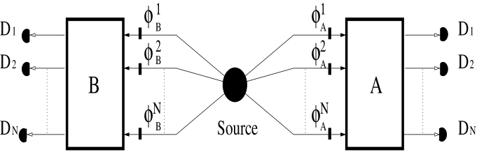
Figure 10.1: The experiment of observer A and B with two maximally entangled qu$N$its. Each of their measuring apparata consist of a set of $N$ phase shifters just in front of an $2N$ port Bell multiport, and $N$ photon detectors $D_{k},D_{l}$ (perfect, in the gedanken situation described here) which register photons in the output ports of the device. The phase shifters serve the role of the devices which set the free macroscopic, classical parameters that can be controlled by the experimenters. The source produces a beam-entangled two qu$N$it state.

Observer A can choose between the non commuting observables $A_{1},A_{2}$ and observer B also can choose between the non commuting observables $B_{1},B_{2}$ (each observable for observer A and B is characterised by some set of local parameters (knobs)) . We assume that the spectrum of each observable consists of $N$ points, which we enumerate by subsequent natural numbers $k,l=1,2,\dots,N$, where index $k$ refers to observer A and index $l$ to observer B. Thus, the observers can perform $2\times 2$ mutually exclusive global experiments.

The quantum probability distribution for the specific pairs of results $k$ and $l$, provided a specific pairs of local observables is chosen ($A_{i}$ and $B_{j}$), will be denoted by $P_{QM}^{F_{N}}(k,l|{A}_{i},{B}_{j})$. In the case considered here the quantum probabilities read

$$P_{QM}^{F_{N}}(k,l|A_{i},B_{j})$$

$$=\frac{1}{N^{2}}F_{N}+(1-F_{N})P_{QM}^{max}(k,l|A_{i},B_{j}),$$ (10.3)

where $P_{QM}^{max}(k,l|A_{i},B_{j})$ is the probability for the given pair of events for the pure maximally entangled state (10.2). Of course, the exact form of $P_{QM}^{max}(k,l|A_{i},B_{j})$ depends on the specific choice of the observables $A_{i},B_{j}$. According to quantum mechanics the set of $4N^{2}$ such probabilities is the only information available to the observers.

10.3 Local realism and joint probability distribution

It is well known (see, e. g. [Fine82], [Peres99]) that the hypothesis of local hidden variables is equivalent to the existence of a (non-negative) joint probability distribution involving all four observables from which it should be possible to obtain all the quantum predictions as marginals. Let us denote this hypothetical distribution by $P_{HV}(k,m;l,n|A_{1},A_{2},B_{1},B_{2})$, where $k$ and $m$, represent the outcome values for observer A observables ($l$ and $n$ for observer B). In quantum mechanics one cannot even define such objects, since they involve mutually incompatible measurements. The local hidden variable probabilities $P_{HV}(...)$ are defined as the marginals

$$P_{HV}(k,l|A_{1},B_{1})=\sum_{m}\sum_{n}P_{HV}(k,m;l,n),$$

$$P_{HV}(k,n|A_{1},B_{2})=\sum_{m}\sum_{l}P_{HV}(k,m;l,n),$$

$$P_{HV}(m,l|A_{2},B_{1})=\sum_{k}\sum_{n}P_{HV}(k,m;l,n),$$

$$P_{HV}(m,n|A_{2},B_{2})=\sum_{k}\sum_{l}P_{HV}(k,m;l,n),$$

(10.4)

where $P_{HV}(k,m;l,n)$ is a short hand notation for $P_{HV}(k,m;l,n|A_{1},A_{2},B_{1},B_{2})$. The $4\times N^{2}$ equations (10.4) form the full set of necessary and sufficient conditions for the existence of local and realistic description of the experiment, i.e., for the joint probability distribution $P_{HV}(k,m;l,n)$. The Bell theorem says that there are quantum predictions, which for $F_{N}$ below a certain threshold cannot be modelled by (10.4), i.e. there exists a critical $F_{N}^{tr}$ below which one cannot have any local realistic model with $P_{HV}(k,l|A_{i},B_{j})=P_{QM}^{F_{N}}(k,l|A_{i},B_{j})$. Our goal is to find observables for the two qu$N$its returning the highest possible critical $F_{N}^{tr}$.

10.4 Linear programming

The set of conditions (10.4) with $P_{QM}^{F_{N}}(k,l|A_{i},B_{j})$ replacing $P_{HV}(k,l|A_{i},B_{j})$ imposes linear constraints on the $N^{4}$ “hidden probabilities” $P_{HV}(k,m;l,n)$ and on the parameter $F_{N}$, which are the nonnegative unknowns. We have more unknowns ($N^{4}+1$) than equations ($4N^{2}$), and we want to find the minimal $F_{N}$ for which the set of constraints can still be satisfied. Then we want to find such local settings characterising the observables that the found minimal $F_{N}$ reaches its highest possible value. From the previous chapters we know how to handle such a problem. We use our sledge hammer: HOPDM 2.30 and the DSM procedures.

10.5 Observables

In our numerical calculations we have used the observables defined by unbiased multiport beamsplitters (for the definition of such a device see chapter devoted to the GHZ paradoxes for qu$N$its).

The quantum prediction for the joint probability $P_{QM}^{max}(k,l|A_{i},B_{j})$ to detect a photon at the $k$-th output of the multiport A characterised by phase shifters $\vec{\phi}^{i}_{A}=(\phi^{1}_{A}(i),...\phi^{N}_{A}(i))$ ($i=1,2$) and another one at the $l$-th output of the multiport B characterised by phase shifters $\vec{\phi}^{j}_{B}=(\phi^{1}_{B}(j),...\phi^{N}_{B}(j))$ ($j=1,2$) for the maximally entangled state (10.2) can be derived from (7.4) with $M=2$ and reads:

$$P_{QM}^{max}(k,l|\vec{\phi}^{i}_{A},\vec{\phi}^{j}_{B})$$

$$=(\frac{1}{N^{3}})\left(N+2\sum^{N}_{m>n}\cos{({\bf\Phi}^{m}_{kl}(ij)-{\bf\Phi}^{n}_{kl}(ij))}\right),$$ (10.5)

where ${\bf\Phi}^{m}_{kl}(ij)\equiv\phi^{m}_{A}(i)+\phi^{m}_{B}(j)+[m(k+l-2)]\frac{2\pi}{N}$. The counts at a single detector, of course, do not depend upon the local phase settings: $P_{QM}(k|A_{i})=P_{QM}(l|B_{j})={1}/{N}$ for all $i,j=1,2$.

10.6 Results

The results are depicted in (10.2).

Figure 10.2: The threshold noise admixture $F_{N}$ versus the dimension of the Hilbert space of qu$N$its. For $N=3$ basing on the computer calculations we were able to find the analytical expression for the threshold noise admixture $F_{3}=\frac{11-6\sqrt{3}}{2}$.

We see that $F_{N}$ continuously increases with growing $N$ exhibiting opposite behaviour to the results obtained in earlier works [Mermin80, Mermin82, Garg82, Peres92, Gisin92, Wódkiewicz94].

For instance, let us compare (10.2) with the results obtained in [Gisin92], which are depicted in (10.3).

Figure 10.3: The threshold noise admixture $F_{N}$ versus the dimension of the Hilbert space of qu$N$its obtained by Gisin and Peres [Gisin92].

We see that for $N=2$ both results are identical. However, starting from $N\geq 3$ the results in (10.3) never exceed the $1-{1\over\sqrt{2}}$. This is due to the fact that in [Gisin92] dichotomic observables were used and the threshold $F_{N}$ was obtained as a condition for violation of CHSH inequality. This behaviour is in agreement with the theorem proved by Tsirelson [Tsirelson80], which states that the CHSH inequality for dichotomic observables can be violated only if $F_{N}$ is lower than $1-{1\over\sqrt{2}}$.

A few words of comment are needed. One may argue that because of a quite large number of local macroscopic parameters (the phases) defining the function to be maximised with the DSM procedure we could have missed the global minimum. While this argument cannot be ruled out in principle, we stress that in that case the ultimate violation would even be larger. This would only strengthen our conclusion that two entangled qu$N$it systems are in stronger conflict with local realism than two entangled qubits.

An important question is whether unbiased multiports provide us with a family of observables in maximal conflict with local realism. For a check of this question we have also calculated the threshold value of $F_{3}$ for the case where both observers apply to the incoming qutrit ($N=3$) the most general unitary transformation belonging to a full SU(3) group (i.e. we have any trichotomic observables on each side). Again we have assumed that each observer chooses between two sets of local settings. However, in this case each set consists of 8 local settings rather than the three (effectively two) in the tritter case. The result appears to be the same as for two tritters, which suggests that tritters (an perhaps generally unbiased multiports) are optimal devices to test quantum mechanics against local realism for $N=3$ (for all $N$).

10.7 Exemplary analytical model for $N=3$

The presented above approach based on the idea of marginals and joint probability distribution compatible with them is the most general one, i.e., it does not assume any symmetries within the tested quantum probabilities (marginals). However, this approach has one drawback. Namely, it involves lots of linear constraints imposed on the joint distribution probability. In the most general case, i.e., when observer A chooses $N_{A}$ observables $A_{i}$ and observer B chooses $N_{B}$ observables $B_{j}$ (each observable has $N$ point spectrum) there are $N_{A}\times N_{B}\times N^{2}$ linear constraints that must be fulfilled by the joint probability distribution (we does not count the constraint that $F_{N}\leq 1$). This considerably lengthens computation time.

On the other hand the quantum probabilities (marginals) that we consider here exhibit some symmetries. Therefore, one can ask the question if, as it has been with two and three maximally entangled qubits (see previous chapters), it is possible to use the properly defined quantum correlation function instead of quantum probabilities.

In this section we show that the answer is yes but only for $N=3$. Considering the quantum correlation function will benefit in calculating the threshold $F_{3}$ for more local settings of the measuring apparata than with the program presented in this chapter.

To this end let us consider two maximally entangled qutrits (qu$N$its with $N=3$) and the quantum correlation function defined in (7.7) with $M=2$ and $N=3$. We remember that it has been obtained by ascribing to the local results of measurements subsequent powers of $\alpha=\exp(\frac{2\pi i}{3})$. We can prove that there is one-to-one equivalence between quantum probabilities (7.4) and the quantum correlation function (7.7).

According to (7.4) for $N=3$ and for any local settings $\vec{\phi}_{A},\vec{\phi}_{B}$ quantum probabilities $P^{QM}(kl|\vec{\phi}_{A},\vec{\phi}_{B})$ can be divided into three groups

$$P_{QM}^{1}=P_{QM}(12)=P_{QM}(21)=P_{QM}(33)$$

$$P_{QM}^{2}=P_{QM}(11)=P_{QM}(23)=P_{QM}(32)$$

$$P_{QM}^{3}=P_{QM}(13)=P_{QM}(31)=P_{QM}(22),$$ (10.6)

where we do not show the dependence on local settings to shorten the notation. This allows us to write the correlation function $E_{QM}(\vec{\phi}^{i}_{A},\vec{\phi}^{j}_{B})$ in the form (for convenience we put $F_{3}=0$)

$$E_{QM}=3(P_{QM}^{1}+\alpha^{2}P_{QM}^{2}+\alpha P_{QM}^{3}),$$ (10.7)

where again we do not show the dependence of the correlation function on local settings. Using the identity ${1\over 3}=P_{QM}^{1}+P_{QM}^{2}+P_{QM}^{3}$ and $\alpha+\alpha^{2}+\alpha^{3}=0$ we arrive at

$${1\over 3}(E_{QM}-1)=(\alpha-1)P_{QM}^{3}-(2+\alpha)P_{QM}^{2},$$ (10.8)

which allows us to express all quantum probabilities through the correlation function (now $F_{3}$ is arbitrary)

$$P_{QM}^{1}={1\over 9}+{2\over 9}ReE_{QM}^{F_{3}}$$

$$P_{QM}^{2}={1\over 9}-{1\over 9}(\sqrt{3}ImE_{QM}^{F_{3}}+ReE_{QM}^{F_{3}})$$

$$P_{QM}^{3}={1\over 9}+{1\over 9}(\sqrt{3}ImE_{QM}^{F_{3}}-ReE_{QM}^{F_{3}}).$$ (10.9)

Therefore, we can apply the approach based on the quantum correlation function presented in the chapter concerning two and three qubits.

For every measurement of the pair of observables $A_{i}$ and $B_{j}$ ($i=1,\dots,N_{a};j=1,\dots,N_{b}$) defined by the tritter and the phase shifters we calculate the quantum correlation function obtaining this way the quantum matrix of predictions $\hat{Q}$ with entries $Q_{ij}(F_{3})=E_{QM}^{F_{3}}(\vec{\phi}^{i}_{A},\vec{\phi}^{j}_{B})$. Note that now the observer A has $N_{A}$ observables to choose from (B has $N_{B}$).

The hidden variable model in this case reads

$$E_{LHV}(\vec{\phi}^{i}_{A},\vec{\phi}^{j}_{B})=\sum_{k=1}^{N^{N_{a}}}\sum_{l=1}^{N^{N_{b}-1}}p_{kl}A(\vec{\phi}^{i}_{A},k)B(\vec{\phi}^{j}_{B},l),$$ (10.10)

where the functions $A(\vec{\phi}^{i}_{A},k)=\alpha^{m}$ and $B(\vec{\phi}^{j}_{B},l)=\alpha^{n}$ ($m,n=1,2,3$). If it is to reproduce the quantum correlation function it must fulfil the following set of $N_{a}\times N_{b}$ linear constraints

$$Q_{ij}(F_{3})=\sum_{k=1}^{N^{N_{a}}}\sum_{l=1}^{N^{N_{b}-1}}p_{kl}A(\vec{\phi}^{i}_{A},k)B(\vec{\phi}^{j}_{B},l).$$ (10.11)

Using HOPDM 2.30 and the DSM we can find the threshold $F_{3}$ still admitting a local and realistic description of the gedanken experiment. The results are identical with those obtained by the previous method. However, since the algorithm is now much faster we were able to perform calculations involving up to 5 different phase settings on each side (i.e. allowing each observer to have a choice of up to 5 different observables to measure). Just as in the two qubit case the optimal $F_{3}$ stayed unchanged at the value obtained for the problem with $N_{a}=N_{b}=2$.

10.7.1 Explicit model for extremal case

Exemplary optimal settings for violation of local realism in the experiment with two qutrits and $N_{a}=N_{b}=2$ are

$$\vec{\phi_{A}}^{1}=(0,\frac{\pi}{3},-\frac{\pi}{3})$$

$$\vec{\phi_{A}}^{2}=(0,0,0)$$

$$\vec{\phi_{B}}^{1}=(0,\frac{\pi}{6},-\frac{\pi}{6})$$

$$\vec{\phi_{B}}^{2}=(0,-\frac{\pi}{6},\frac{\pi}{6}).$$ (10.12)

For such settings the quantum matrix $\hat{Q}$ (with $F_{3}=0$) reads

$$\hat{Q}=\left(\begin{array}[]{cc}Q_{1}&Q_{1}^{*}\\ Q_{2}&Q_{1}\\ \end{array}\right),$$ (10.15)

where $Q_{1}=\frac{2\sqrt{3}+1}{6}-i\frac{2-\sqrt{3}}{6}$ and $Q_{2}=-{1\over 3}(1+2i)$. Please, note that the all entries of (10.15) have the same modulus equal $\frac{\sqrt{5}}{3}$.

The hidden variables can only reproduce the matrix of correlation function given by $(1-F_{3})\hat{Q}$ with $F_{3}\leq\frac{11-6\sqrt{3}}{2}$. For the threshold maximal $F_{3}$ the explicit model is given by

$$\hat{Q}^{F_{3}}=p\left(\begin{array}[]{cc}\alpha^{3}&\alpha^{3}\\ \alpha^{3}&\alpha^{3}\\ \end{array}\right)+p\left(\begin{array}[]{cc}\alpha^{2}&\alpha^{3}\\ \alpha^{2}&\alpha^{3}\\ \end{array}\right)+$$ (10.20)

$$p\left(\begin{array}[]{cc}\alpha^{3}&\alpha^{3}\\ \alpha^{2}&\alpha^{2}\\ \end{array}\right)+p\left(\begin{array}[]{cc}\alpha^{3}&\alpha\\ \alpha^{2}&\alpha^{3}\\ \end{array}\right)+$$ (10.25)

$$q\left(\begin{array}[]{cc}\alpha^{3}&\alpha^{2}\\ \alpha&\alpha^{3}\\ \end{array}\right)+q\left(\begin{array}[]{cc}\alpha&\alpha^{3}\\ \alpha^{2}&\alpha\\ \end{array}\right)=(1-F_{3})\hat{Q},$$ (10.30)

where $p=\frac{4-2\sqrt{3}}{3}$, $q=\frac{8\sqrt{3}-13}{6}$.

This model has to be understood in the following way. Consider the first term. The rank-one matrix

$$\left(\begin{array}[]{cc}\alpha^{3}&\alpha^{3}\\ \alpha^{3}&\alpha^{3}\\ \end{array}\right)$$ (10.33)

can be factorised into column and row matrices built out of powers of $\alpha$, in the following three ways:

$$\left(\begin{array}[]{cc}\alpha^{3}&\alpha^{3}\\ \alpha^{3}&\alpha^{3}\\ \end{array}\right)=\left(\begin{array}[]{c}\alpha^{3}\\ \alpha^{3}\end{array}\right)\left(\begin{array}[]{c}1\\ 1\end{array}\right)^{T}=\left(\begin{array}[]{c}\alpha^{2}\\ \alpha^{2}\end{array}\right)\left(\begin{array}[]{c}\alpha\\ \alpha\end{array}\right)^{T}=\left(\begin{array}[]{c}\alpha\\ \alpha\end{array}\right)\left(\begin{array}[]{c}\alpha^{2}\\ \alpha^{2}\end{array}\right)^{T}.$$ (10.48)

Therefore with probability $p^{\prime}={1\over 3}p$ each of this factorisations is present in the model of $\hat{Q}^{F_{3}}$ (compare (10.10) and (10.11)).

10.8 Conclusions

It is evident, that indeed two entangled qu$N$its violate local realism stronger than two entangled qubits, and that the violation increases with $N$. It is important to stress that the values were obtained using four independently written codes, one of them employing a different linear optimisation procedure (from the NAG Library).

It is interesting to compare our results with the limit [Horodecki99] for the non separability of the density matrices [Werner89] of the two entangled systems. The fact that this limit, $\frac{N}{N+1}$, is always higher than ours indicates that that requirement of having local quantum description of the two subsystems is a much more stringent condition than our requirement of admitting any possible local realistic model.

It will be interesting to consider within our approach different families of states, generalisations to more than two qu$N$its, extensions of the families of observables, to see if a wider choice of experiments than can be performed on one side (i.e., more than two) can lead to even stronger violations of local realism, and finally to see experimental realizations of such schemes.

Finally we should mention that this approach can be extended to the research into the threshold efficiency of detectors for such experiments. The computer program for imperfect detectors has been already written.

Appendix A Proof of equivalence of the existence of local hidden variables and a joint probability distribution for incompatible measurements

This appendix is a re-derivation of known results (see e.g. [Fine82]).

We consider the experiment with two observers A and B. Observer A can choose to measure $N_{A}$ observables $A_{i}$ ($i=1,2,\dots,N_{A}$) whereas observer can choose to measure $N_{B}$ observables $B_{j}$ ($j=1,2,\dots,N_{B}$). In the measurement of the observable $A_{i}$ observer A can obtain $N$ results, which we denote by $k_{i}$ ($i=1,\dots,N$). Similarly, in the measurement of the observable $B_{j}$ observer B can obtain $N$ results, which we denote by $l_{j}$ ($j=1,\dots,N$). In the experiment the observers can only measure joint probabilities $P(k_{i},l_{j}|A_{i},B_{j})$, i.e., probabilities of obtaining the result $k_{i}$ when measuring the observable $A_{i}$ and the result $l_{j}$ when measuring the observable $B_{j}$.

First, let us show that the existence of stochastic local hidden variables recovering the marginals $P(k_{i},l_{j}|A_{i},B_{j})$ implies the existence of a joint probability distribution

$$P_{HV}(k_{1},\dots,k_{N_{A}},l_{1},\dots,l_{N_{B}}|A_{1},\dots,A_{N_{A}},B_{1},\dots,B_{N_{B}})$$ (A.1)

compatible with the given marginals. The existence of local hidden variable space $\Lambda$ and the ”hidden” probabilities $P_{i}(k_{i}|\lambda,A_{i})$ and $P_{j}(l_{j};\lambda,B_{j})$ (see (2.13)) allows one to define the joint probability distribution (A.1) in the following way

$$P_{HV}(k_{1},\dots,k_{N_{A}},l_{1},\dots,l_{N_{B}}|A_{1},\dots,A_{N_{A}},B_{1},\dots,B_{N_{B}})$$

$$=\int_{\Lambda}d\rho(\lambda)\prod_{i=1}^{N_{A}}P_{i}(k_{i}|\lambda,A_{i})\prod_{j=1}^{N_{B}}P_{j}(l_{j}|\lambda,B_{j}).$$ (A.2)

It is evident that (A.2) returns as marginals $P(k_{i},l_{j}|A_{i},B_{j})$.

Now let us assume that (A.1) exists and is compatible with the marginals $P(k_{i},l_{j}|A_{i},B_{j})$ We can define the local hidden variables as follows. To each sequence of possible results $(\tilde{k}_{1},\tilde{k}_{2},\dots,\tilde{k}_{N_{A}},\tilde{l}_{1},\tilde{l}_{2},\dots,\tilde{l}_{N_{B}})$ we ascribe a hidden variable, which we denote as $\lambda(\tilde{k}_{1},\tilde{k}_{2},\dots,\linebreak\tilde{k}_{N_{A}},\tilde{l}_{1},\tilde{l}_{2},\dots,\tilde{l}_{N_{B}})$. Therefore, the local hidden variable space $\Lambda$ consists of $N^{N_{A}+N_{B}}$ different hidden variables. On this space we define the discrete probability distribution of local hidden variables $\rho(\lambda)$ in the following way

$$\rho(\lambda(\tilde{k}_{1},\tilde{k}_{2},\dots,\tilde{k}_{N_{A}},\tilde{l}_{1},\tilde{l}_{2},\dots,\tilde{l}_{N_{B}}))$$

$$=P_{HV}(\tilde{k}_{1},\dots,\tilde{k}_{N_{A}},\tilde{l}_{1},\dots,\tilde{l}_{N_{B}}|A_{1},\dots,A_{N_{A}},B_{1},\dots,B_{N_{B}}).$$ (A.3)

The hidden probabilities $P_{i}(k_{i}|\lambda,A_{i})$ and $P_{j}(l_{j}|\lambda,B_{j})$ we define as

$$P_{i}(k_{i}|\lambda(\tilde{k}_{1},\tilde{k}_{2},\dots,\tilde{k}_{N_{A}},\tilde{l}_{1},\tilde{l}_{2},\dots,\tilde{l}_{N_{B}}),A_{i})=\delta_{\tilde{k}_{i},k_{i}}$$

$$P_{j}(l_{j}|\lambda(\tilde{k}_{1},\tilde{k}_{2},\dots,\tilde{k}_{N_{A}},\tilde{l}_{1},\tilde{l}_{2},\dots,\tilde{l}_{N_{B}}),B_{j})=\delta_{\tilde{l}_{j},l_{j}},$$ (A.4)

where $\delta$ denotes the Kronecker delta function. Then the marginals are recovered in the following way

$$P(k_{i},l_{j}|A_{i},B_{j})$$

$$=\sum_{\lambda}\rho(\lambda(\tilde{k}_{1},\tilde{k}_{2},\dots,\tilde{k}_{N_{A}},\tilde{l}_{1},\tilde{l}_{2},\dots,\tilde{l}_{N_{B}}))\delta_{\tilde{k}_{i},k_{i}}\delta_{\tilde{l}_{j},l_{j}},$$ (A.5)

where we sum over all $N^{N_{A}+N_{B}}$ hidden variables $\lambda$. Using the above definitions (A.5) can be rewritten as

$$P(k_{i},l_{j}|A_{i},B_{j})=\sum_{\lambda}\rho(\lambda)P_{i}(k_{i}|\lambda,A_{i})P_{j}(l_{j}|\lambda,B_{j}),$$ (A.6)

i.e. we have a typical structure of a local hidden variable model (for hidden variables forming a discrete set).

Bibliography

- [Aerts99] S. Aerts, P. Kwiat, J. -Å. Larsson, and M. Żukowski, Phys. Rev. Lett. 83, 2872 (1999).
- [Agarwal93] G. S. Agarwal, Phys.Rev. A 47, 4608 (1993).
- [Ardehali91] M. Ardehali, Phys. Rev. D 44, 3336 (1991).
- [Ardehali92] M. Ardehali, Phys. Rev. A 46, 5375 (1992)
- [Aspect82] A. Aspect, J. Dalibard, and G. Roger, Phys. Rev. Lett. 49, 1804 (1982).
- [Belinfante73] F. J. Belinfante, Asurvey of Hidden-Variables Theories, Oxford, Pergamon, 1973.
- [Bell64] J. Bell, Physics 1, 195 (1964).
- [Bell66] J. S. Bell, Rev. Mod. Phys. 38, 447 (1966).
- [Bell87] J. S. Bell. Speakable and Unspeakable in Quantum Mechanics. Camridge UP, Cambridge, 1987.
- [Bennett84] C. H. Bennett and G. Brassard, in Proceedings of the IEEE International Conference on Computers, Systems, and Signal Processing, Bangalore, India (IEEE, New York, 1984), p. 175.
- [Bennett93] C. Bennett, G. Brassard, C. Crepeau, R. Jozsa, A. Peres and W. Wooters, Phys. Rev. Lett. 70, 1895 (1993).
- [Belinski93] A. V. Belinskii and D. N. Klyshko, Phys. Usp. 36, 653 (1993).
- [Bohm51] D. Bohm. Quantum Theory, Prentice Hall, Englewood Cliffs, 1951.
- [Bohm52] D. Bohm, Phys. Rev. 85, 166 (1952).
- [Bose98] S. Bose, V. Vedral, P. L. Knight, Phys. Rev. A 57, 822 (1998).
- [Bouwmeester97] D. Bouwmeester, J.-W. Pan, K. Mattle, M. Eible, H. Weinfurter and A. Zeilinger, Nature 390 575 (1997).
- [Bouwmeester98] D. Bouwmeester, K. Mattle, J.-W. Pan, H. Weinfurter, A. Zeilinger and M. Żukowski, Appl. Phys. B, 67 749 (1998).
- [Bouwmeester99] D. Bouwmeester, Jian-Wei Pan, M. Daniell, H. Weinfurter and A. Zeilinger, Phys. Rev. Lett. 82, 1345 (1999).
- [Braunstein89] S. L. Braunstein and C. M. Caves, Ann. Phys. (NY) 202, 22 (1990).
- [Casado97] A. Casado, A. Fernandez-Rueda, T. W. Marshall, R. Risco-Delgado and E. Santos, Phys. Rev. A 55, 3879 (1997).
- [Clauser69] J. F. Clauser, M. A. Horne, A. Shimony and R. A. Holt, Phys. Rev. Lett. 23, 880 (1969).
- [Clauser74] J.F Clauser and M. A. Horne, Phys. Rev. D 10, 526 (1974).
- [Clauser78] J. F. Clauser and A. Shimony, Rep. Prog. Phys. 41, 1881 (1978).
- [Deutsch89] D. Deutsch, Proc. R. Soc. London A 425, 73 (1989).
- [Eckert91] A. K. Ekert, Phys. Rev. Lett. 67, 661 (1991).
- [Einstein35] A. Einstein, B. Podolsky and N. Rosen, Phys. Rev. 47, 777 (1935).
- [Feynman82] R. Feynman, Int. J. Theor. Phys. 21, 219 (1982).
- [Fine82] A. Fine, Phys. Rev. Lett. 48, 291 (1982).
- [Freedman72] S. J. Freedman and J. F. Clauser, Phys. Rev. Lett. 28, 938 (1972).
- [Garg82] A. Garg and N. D. Mermin, Phys. Rev Lett. 49, 901 (1982).
- [Garg85] A. Garg and N. D. Mermin, Phys. Rev. D 35, 3832 (1985).
- [Garg87] A. Garg, N. D. Mermin, Phys. Rev. D 35, 3638 (1987).
- [Garuccio80] A. Garuccio and F. Selleri, Found. Phys. 10, 209 (1980).
- [Garuccio94] L. De Caro and A. Garuccio, Phys. Rev. A 50, R2803 (1994).
- [Gass75] S. I. Gass Linear programming 4th ed. New York: McGraw-Hill 1975.
- [Gisin92] N. Gisin and A. Peres, Phys. Lett. A 162, 15 (1992).
- [Gisin99] N. Gisin, Phys. Lett. A 260, 1 (1999).
- [Gleason57] A. M. Gleason, J. Math. and Mech. 6, 885 (1957).
- [Gondzio95] J. Gondzio, European Journal of Operational Research 85, 221 (1995); J. Gondzio, Computational Optimization and Applications 6, 137 (1996).
- [Greenberger89] D. M. Greenberger, M. A. Horne and A. Zeilinger, in Bell’s Theorem, Quantum Theory, and Conceptions of the Universe, edited by Kafatos, M. (Kluwer Academics, Dordrecht, The Netherlands,1989), p. 73.
- [Greenberger90] D. M. Greenberger, M. Horne, A. Shimony and A. Zeilinger Am. J. Phys. 58, 1131 (1990).
- [Hagley97] E. Hagley, X. Maitre, G. Nogues, C. Wunderlich, M. Brune, J. M. Raimond, and S. Haroche, Phys. Rev. Lett. 79, 1 (1997).
- [Hong85] C. Hong, L. Mandel, Phys. Rev. A 31, 2409, (1985).
- [Hong87] C. K. Hong, Z. Y. Ou and L. Mandel, Phys. Rev. Lett. 59, 2044 (1987).
- [Horne85] M. A. Horne and A. Zeilinger, in Symposium on Foundations of Modern Physics, eds. P. Lahti and P. Mittelstaedt (World Sc., Singapore, 1985).
- [Horne89] M. A. Horne, A. Shimony and A. Zeilinger, Phys. Rev. Lett. 62, 2209 (1989).
- [Horodecki95] R. Horodecki, P. Horodecki and M. Horodecki, Phys. Lett. A 200, 340 (1995).
- [Horodecki96] M. Horodecki, P. Horodecki, and R. Horodecki, Phys. Lett. A 223, 1 (1996).
- [Horodecki99] M. Horodecki and P. Horodecki, Phys. Rev. A 59, 4206 (1999).
- [Ivanovic81] I. D. Ivanovic, J. Phys. A 14, 3241 (1981).
- [Jex95] I. Jex, S. Stenholm and A. Zeilinger, Opt. Comm. 117, 95 (1995).
- [Jaeger93] G. Jaeger, M. A. Horne and A. Shimony, Phys. Rev. A, 48, 1023 (1993).
- [Klyshko88] D. N. Klyshko, Phys. Lett. A 132, 299 (1988).
- [Kochen67] S. Kochen and E. Specker, J. Math. Mech. 17, 59 (1967).
- [Kwiat93] P. G. Kwiat, A. M. Steinberg and R. Y. Chiao, Phys. Rev. A 47, R2472 (1993)
- [Kwiat94] P. G. Kwiat, P. E. Eberhard, A. M. Steinberg and R. Y. Chiao, Phys. Rev. A 49, 3209 (1994).
- [Kwiat95] P. G. Kwiat, Phys. Rev. A 52, 3380 (1995).
- [Larsson99] J.-Å. Larsson, Phys. Lett. A 256, 245 (1999).
- [Mattle95] C. Mattle, M. Michler, H. Weinfurter, A. Zeilinger and M. Żukowski, Appl. Phys. B 60, S111 (1995).
- [Mattle96] K. Mattle, H. Weinfurter, P. G. Kwiat and A. Zeilinger, Phys. Rev. Lett. 76, 4656 (1996).
- [Mermin80] N. D. Mermin, Phys. Rev. D 22, 356 (1980).
- [Mermin82] N. D. Mermin and G. M. Schwarz, Found. Phys. 12, 101 (1982).
- [Mermin90a] N. D. Mermin Physics Today, p. 9 (June 1990).
- [Mermin90b] N. D. Mermin, Phys. Rev. Lett. 65, 1838 (1990).
- [Michler96] M. Michler, K. Mattle, H. Weinfurter and A. Zeilinger, Phys. Rev. A 53, R1209 (1996).
- [Michler00] M. Michler, H. Weinfurter, M. Żukowski, Phys. Rev. Lett. 84, 5427 (2000).
- [Nelder65] J. A. Nelder and R. Mead, Computer Journal 7, 308 (1965).
- [Ou88] Z. Y. Ou and L. Mandel, Phys. Rev. Lett. 61, 50 (1988).
- [Pan98] J. W. Pan, D. Bouwmeester, H. Weinfurter, A. Zeilinger, Phys. Rev. Lett. 80, 3891 (1998).
- [Peres92] A. Peres, Phys. Rev. A 46, 4413 (1992).
- [Peres96] A. Peres, Phys. Rev. Lett. 77, 1413 (1996).
- [Peres99] A. Peres, Found. Phys. 29, 589 (1999).
- [Pittman95] T. B. Pittman, Y. H. Shih, A. V. Sergienko and M. H. Rubin, Phys. Rev. A 51, 3495 (1995).
- [Popescu97] S. Popescu, L. Hardy and M. Żukowski, Phys. Rev. A 56, R4353 (1997).
- [Rarity90] J. G. Rarity and P. R. Tapster, Phys. Rev. Lett. 64, 2495 (1990).
- [Reck94] M. Reck, A. Zeilinger, H. J. Bernstein and P. Bertani, Phys. Rev. Lett. 73, 58 (1994).
- [Reck96] M. Reck, PhD Thesis (supervisor: A. Zeilinger) (University of Innsbruck, 1996, unpublished).
- [Redhead87] M. Redhead. Incompletness, Nonlocality, and Realism. A prolegomenon to the philosophy of quantum mechanics. Clarendon Press, Oxford, 1987.
- [Roy91] S. M. Roy and V. Singh, Phys. Rev. Lett. 67, 2761 (1991).
- [Santos92] E. Santos, Phys. Rev. A 46, 3646 (1992).
- [Schröedinger35] E. Schrödinger. The present situation in quantum mechanics. In J. Wheeler and W. Żurek, editors, it Quantum Theory and Measurement, p. 152. Princeton University Press, 1983.
- [Schwinger60] J. Schwinger, Proc. Nat. Acad. Sc. 46, 570 (1960).
- [Selleri88] Quantum MechanicsVersus Local Realism. The Einstein-Podolsky-Rosen Paradox. Edited by F. Selleri. Plenum Press, New York, 1988.
- [Shih88] C. O. Alley and Y. H. Shih, Phys. Rev. Lett. 61, 2921 (1988).
- [Stapp77] H. Stapp, Nuovo Cimento 40B, 191 (1977).
- [Tapster94] P. R. Tapster, J. G. Rarity, and P. C. M. Owens, Phys. Rev. Lett. 73, 1923 (1994).
- [Tittel98] W. Tittel, J. Brendel, H. Zbinden, and N. Gisin, Phys. Rev. Lett. 81, 3563 (1998).
- [Tsirelson80] B. S. Cirel’son, Lett. Math. Phys. 4, 93 (1980).
- [Wódkiewicz91] C. Su and K. Wódkiewicz, Phys. Rev. A 44, 6097 (1991).
- [Wódkiewicz94] K. Wódkiewicz, Acta Phys. Pol. 86, 223 (1994).
- [Wódkiewicz95] K. Wódkiewicz, Phys. Rev A 51, 2785 (1995).
- [Weihs96] G. Weihs, M. Reck, H. Weinfurter, A. Zeilinger, Opt. Lett., 21, 302 (1996).
- [Weihs98] G. Weihs, T. Jennewein, Ch. Simon, H. Weinfurter and A. Zeilinger, Phys. Rev. Lett. 81, 5039 (1998).
- [Werner89] R. Werner, Phys. Rev. A 40, 4277 (1989).
- [Wigner70] E. P. Wigner, Am. J. Phys. 38, 1005 (1970).
- [Wooters86] W. K. Wooters, Found. Phys. 16, 391 (1986).
- [Yurke92] B. Yurke and D. Stoler, Phys. Rev. A 46 2229 (1992); Phys. Rev. Lett., 68 1251 (1992).
- [Zeilinger86] A. Zeilinger, Am. J. Phys 49, 882 (1981).
- [Zeilinger93] A. Zeilinger, H. J. Bernstein, D. M. Greenberger, M. A. Horne, and M. Żukowski, in QuantumControl and Measurement, eds. H. Ezawa and Y. Murayama (Elsevier, 1993).
- [Zeilinger94] A. Zeilinger, M. Żukowski, M. A. Horne, H. J. Bernstein and D. M. Greenberger, in Quantum Interferometry, eds. F. DeMartini, A. Zeilinger, (World Scientific, Singapore, 1994).
- [Żukowski88] M. Żukowski and J. Pykacz, Phys. Lett. A 127, 1 (1988).
- [Żukowski93a] M. Żukowski, A. Zeilinger, M. A. Horne and A. K. Ekert, Phys. Rev. Lett. 71, 4287 (1993).
- [Żukowski93b] M. Żukowski, Phys. Lett. A, 177, 290 (1993)
- [Żukowski95] M. Żukowski, A. Zeilinger, H. Weinfurter: Ann. N. Y. Acad. Science 755, 91 (1995).
- [Żukowski97b] M. Żukowski, A. Zeilinger, M. A. Horne, Phys. Rev. A 55, 2564 (1997).
- [Żukowski99] M. Żukowski, A. Zeilinger, M. A. Horne and H. Weinfurter, Int. J. Theor. Phys. 38, 501 (1999).
- [Żukowski91] M. Żukowski, Phys. Lett. A 177, 290 (1991).
- [vonNeumann32] J. v. Neumann, Mathematishe Grundlagender Quantenmechanik. Springer, Berlin, 1932.
- [1] M. Żukowski, D. Kaszlikowski and E. Santos, Phys. Rev. A 60, R2614 (1999).
- [2] M. Żukowski and D. Kaszlikowski, Acta Phys. Slov. 49, 621 (1999).
- [3] M. Żukowski and D. Kaszlikowski, Phys. Rev. A, 56, R1682 (1997).
- [4] D. Kaszlikowski and M. Żukowski, Phys. Rev. A 61, 022114 (2000).
- [5] M. Żukowski and D. Kaszlikowski, Phys. Rev. A 59, 3200 (1999).
- [6] M. Żukowski and D. Kaszlikowski, Vienna Circle Yearbook vol. 7, editors D. Greenberger, W. L. Reiter, A. Zeilinger, Kluwer Academic Publishers, Dortrecht (1999).
- [7] M. Żukowski, D. Kaszlikowski, A. Baturo and J. -A. Larsson, quant-ph/9910058
- [8] D. Kaszlikowski, P. Gnacinski, M. Żukowski, W. Miklaszewski and A. Zeilinger, quant-ph/0005028