Phase diffusion as a model for coherent suppression of tunneling in the presence of noise

Abstract

We study the stabilization of coherent suppression of tunneling in a driven double-well system subject to random periodic $\delta-$function “kicks”. We model dissipation due to this stochastic process as a phase diffusion process for an effective two-level system and derive a corresponding set of Bloch equations with phase damping terms that agree with the periodically kicked system at discrete times. We demonstrate that the ability of noise to localize the system on either side of the double-well potenital arises from overdamping of the phase of oscillation and not from any cooperative effect between the noise and the driving field. The model is investigated with a square wave drive, which has qualitatively similar features to the widely studied cosinusoidal drive, but has the additional advantage of allowing one to derive exact analytic expressions.

I Introduction

Coherent suppression of tunneling is a localization effect that occurs when a potential with multiple minima is exposed to a periodic drive in a specific parameter regime Dun86 ; Gro91 ; Hol92 . In their original paper, Grossman et. al. Gro91 examined this phenomena in the context of a quartic double-well potential driven by a strong cosinusoidal force. It was later shown that the essence of this effect could be described by the two lowest energy eigenstates corresponding to the symmetric $|S\rangle$, and antisymmetric $|A\rangle$, states of the ground state doublet. This approximation is valid if the drive strength, drive frequency and energy splitting are small compared to the energy spacing between the average energy of the ground doublet and the higher energy levels Llo92 . The two level approximate Hamiltonian for this system written in a basis of left and right states, $|L,R\rangle=(|S\rangle\mp|A\rangle)/\sqrt{2}$, is described by a bare tunneling system with an energy splitting $A_{x}$ and a cosine driving force with amplitude $A_{z}$ and frequency $\omega_{d}$,

$$\hat{H}(t)=\frac{A_{x}}{2}\hat{\sigma}_{x}+\frac{A_{z}}{2}\cos(\omega_{d}t)\hat{\sigma}_{z}.$$ (1)

A complete suppression of tunneling occurs when the drive amplitude is much larger than the energy splitting ($A_{z}\gg A_{x}$) and the ratio of the drive amplitude to the drive frequency is equal to a root of the zero order Bessel function Llo92 . This absence of coherent oscillation is due to the two Floquet states of the driven system becoming exactly degenerate Gro93 .

A counterintuitive effect Gro93 ; Dit93 ; Koh98 occurs when dissipation is added to this system. This can be modeled by the addition of a stochastic $\delta$-function kick, which is applied periodically Gro93 . When the ratio of the amplitude to the frequency of the periodic driving field is near but not equal to the Bessel root condition in the absence of noise, coherent oscillations between the left and right wells proceed at a modified tunneling rate corresponding to the quasienergy splitting (See Fig. 1). At first, the effect of noise is to destroy coherent oscillations causing the system to evolve into a 50/50 mixture of left and right wells. However, increasing the noise strength appears to have a stabilizing effect on coherent suppression of tunneling Gro93 ; Dit93 causing the system to remain in the well corresponding to its initial state. This seems surprising because the condition for coherent suppression of tunneling depends on the state of the system being in a stationary superposition of the two degenerate Floquet states for all times whereas dissipation generally tends to destroy quantum coherence. However, we will demostrate that this localization effect can be understood intuitively as arising from strong damping of the phase of oscillation. This has been previously pointed out by Makarov Mak93 using a semiclassical quantization scheme to establish a correspondence between a classically driven two-level system and the spin-boson problem. Standard treatments of dissipation based on the master equation of a reduced density operator after tracing over a large reservoir Dit93 ; Mak93 ; Mak95 can obscure the physical content of this localization phenomena. Our treatment uses a simplified model based on a damping due to phase diffusion from random classical kicks. This model corresponds to the regime of weak coupling to a classical noise reservoir Leg87 ; Mak93 ; Mak95 . From this we derive a detailed and exact expression for the tunneling oscillations that gives a clear interpretation of this phenomena that excludes any cooperative effects between the noise and the driving field.

Dissipation in driven two level systems has been extensively studied Gro93 ; Dit93 ; Koh98 ; Mak93 ; Mak95 ; Wei99 ; Dak94 ; Gri95 ; Gri96a ; Mak97 ; Neu97 ; Gri97 ; For99 ; Sto99 because this model provides a realistic paradigm for understanding a variety of physical systems. For example this model can be used to describe charge oscillations in semiconductor double wells Bav92 ; Dak93a ; Dak93b , magnetic flux dynamics in superconducting quantum interference devices (SQUIDs) Han91 , condensed phase electron and proton reactions Mor93 ; Fle90 ; Ben94 and strong field spectroscopy Cuk98 ; Mor99 . Recently, quantum tunneling over mesoscopic distances and the generation of mesoscopic superposition states has been realized in an optical lattice of double wells Hay00 . This system is ideally suited for the study of the driven double well in the presence of dissipation given the large degree of experimental control one has over the system Deu98 . For example the energy barrier and energy assymmetry can be dynamically controlled through laser beam configuration and externally applied magnetic fields. Furthermore, this system can operate in an essentially dissipation free environment when the lattice lasers are sufficiently far detuned from the atomic resonance. Dissipation can then be reintroduced into the system in the form of well-controlled fluctuations in the potential Deu98 ; Deu00 .

In this paper we replace the cosine drive field with a periodic square wave drive field. Our Hamiltonian reads,

$$\hat{H}(t) = \frac{A_{x}}{2}\hat{\sigma}_{x}+\frac{A_{z}}{2}\Lambda(\omega_{d}t)\hat{\sigma}_{z},$$

$$\Lambda(\omega_{d}t) = \left\{\begin{array}[]{ll}+1&\mbox{ for }0\leq\mbox{mod}_{\tau_{d}}(t)<\frac{\tau_{d}}{2}\\ -1&\mbox{ for }\frac{\tau_{d}}{2}\leq\mbox{mod}_{\tau_{d}}(t)<\tau_{d},\end{array}\right.$$ (5)

where $\tau_{d}=\frac{2\pi}{\omega_{d}}$ is the drive period. This drive has similar qualitative features to the sinusoidal force. For instance, the condition for coherent suppression of tunneling occurs when the ratio of the amplitude to the frequency of the drive is equal to an integer rather than a root of the zero order Bessel function. However, this Hamiltonian has the advantage that one can derive analytic results without making approximations that are common when analyzing sinusoidal drives. The paper is organized as follows. In Sec. II we present an effective magnetic field formalism in the Floquet basis showing how one can describe the tunneling system with a set of Bloch equations associated with spin precession about a fictitous static magnetic field. In Sec. III we show how one can use a phase diffusion model to describe the dissipation in terms of dephasing terms added to the Bloch equations and we present results that compare numerical simulations to analytic expressions. In Sec. IV we summarize our results.

II The effective magnetic field in the Floquet basis

As discussed above, we simplify the problem of a tunneling wave packet in a double well by considering the problem restricted to the two lowest energy eigenstates. Because this is a two-level system one can visualize the dynamics geometrically on the Bloch sphere with spin up and spin down along the quantization axis $\mathbf{\hat{z}}$ corresponding to the localized $|L\rangle$ and $|R\rangle$ states respectively. According to the bare Hamiltonian, the first term in Eq. (2), tunneling on the Bloch sphere is pictured as the Larmour precession of a Bloch vector, $\mathbf{s}$, about a static magnetic field in the $\mathbf{\hat{x}}$ direction with a frequency $\omega_{L}=A_{x}$ ($\hbar=1$). When a drive is added to the tunneling system, such as the square wave drive given in Eq. (2), the Hamiltonian becomes time dependent. In general, a drive term causes trajectories to explore the entire Bloch sphere in a complicated fashion (See Fig. 2a). However, when the ratio of the amplitude to the frequency of the drive is an integer and $A_{z}\gg A_{x}$, one finds that the trajectories on the Bloch sphere form closed “loops” near the top (or bottom) of the Bloch sphere which correspond to the quantum system remaining localized in the $|L\rangle$ (or $|R\rangle$) state (See Fig. 2b). This is the coherent suppression of tunneling. Note that if the condition $A_{z}\gg A_{x}$ (typically $A_{z}/A_{x}\gtrsim 5$) is not satisfied then the system can still form closed trajectories but they do not stay “near” the top or bottom of the Bloch sphere and hence are not localizing.

According to the Floquet theorem Shi65 ; Gri98 , a system with a Hamiltonian that is periodic in time, $\hat{H}(t+\tau_{d})=\hat{H}(t)$, has solutions to the Schrödinger equation, $|\varepsilon_{j}\rangle$, which are eigenfunctions of the single period time propagator or Floquet operator, ($\hbar=1$)

$$\hat{U}(\tau_{d},0)=\hat{\mathcal{T}}\exp\Bigl{(}-i\int_{0}^{\tau_{d}}dt\hat{H}(t)\Bigr{)}$$ (6)

where $\hat{\mathcal{T}}$ denotes the time-ordering operator. The eigenvalues of this propagator are given by

$$\hat{U}(\tau_{d},0)|\varepsilon_{j}\rangle=\exp(-i\varepsilon_{j}\tau_{d})|\varepsilon_{j}\rangle,$$ (7)

where $\varepsilon_{j}$ is a quasienergy which belongs to a family of quasienergies such that $\varepsilon_{j}+k\omega_{d}$ (where $k$ is an integer) belongs to the same physical state. Quasienergies can be uniquely defined by requiring them to continuously approach the energies of the time independent Hamiltonian as the periodic part vanishes. Because the Floquet states are stationary states at integer multiples of $\tau_{d}$, we restrict time to these discrete values. In this stroboscopic picture of the dynamics, the Floquet states evolve like energy eigenstates for a time-independent Hamiltonian with the quasienergies playing the role of energies.

For a two-level system we denote the Floquet states $\{|\varepsilon_{-}\rangle,|\varepsilon_{+}\rangle\}$. Writing the single period time propagator in the Floquet basis and neglecting global phase factors gives,

$$\hat{U}(\tau_{d},0)=\hat{1}\cos\Bigl{(}\frac{\Delta\varepsilon\tau_{d}}{2}\Bigr{)}-i(\mathbf{\hat{\vec{\sigma}}}\cdot\mathbf{\hat{e}}_{F})\sin\Bigl{(}\frac{\Delta\varepsilon\tau_{d}}{2}\Bigr{)},$$ (8)

where $\Delta\varepsilon=\varepsilon_{+}-\varepsilon_{-}$ is the quasienergy splitting and the quantization direction, $\mathbf{\hat{e}}_{F}$, is chosen along $|\varepsilon_{+}\rangle$. We see that the application of the single period time propagator can be thought of as a rotation about an effective magnetic field, $\mathbf{B}_{F}=\Delta\varepsilon\;\mathbf{\hat{e}}_{F}$. Because the single period time propagator commutes with itself at integer multiples of the drive period, the unitary time propagator after $\ell$ drive periods is found from $\ell$ applications of the single period time propagator, $\hat{U}(\ell\tau_{d},0)=\hat{U}(\tau_{d},0)^{\ell}$ ($\ell=0,1,2,\cdots$). The end result of utilizing this representation is that one can replace the continuous dynamics of a time dependent Hamiltonian with a discrete dynamics associated with a time independent Hamiltonian described by spin precession about a fictitous static magnetic field (See Fig 3). This transformation is not an approximation, like the well known rotating wave approximation; the two pictures are in exact agreement at these discrete times. However, the time resolution of the Bloch trajectories is fundamentally limited by the drive period because this quasistatic picture does not contain information about time scales shorter than the drive period.

For the specific case of the square wave drive the time dependent Hamiltonian can be decomposed into two time independent Hamiltonians, $\hat{H}_{\pm}=\frac{A_{x}}{2}\hat{\sigma}_{x}\pm\frac{A_{z}}{2}\hat{\sigma}_{z}$. According to Eq. (2), the single period unitary operator can be easily contructed by multiplying the two half period unitaries,

$$\hat{U}(\tau_{d},0) = \exp\Bigl{(}-i\hat{H}_{-}\frac{\tau_{d}}{2}\Bigr{)}\exp\Bigl{(}-i\hat{H}_{+}\frac{\tau_{d}}{2}\Bigr{)}$$ (9b)

$$= \Bigl{(}1-2\sin^{2}(\frac{\phi}{2})\sin^{2}(\theta)\Bigr{)}\hat{1}$$

$$-\Bigl{(}2i\sin(\frac{\phi}{2})\cos(\frac{\phi}{2})\sin(\theta)\Bigr{)}\hat{\sigma}_{x}$$

$$+\Bigl{(}2i\sin^{2}(\frac{\phi}{2})\sin(\theta)\cos(\theta)\Bigr{)}\hat{\sigma}_{y},$$

where $\phi=\sqrt{A_{x}^{2}+A_{z}^{2}}\;\tau_{d}$ and $\tan(\theta)=A_{z}/A_{x}$. The effective magnetic field for the square wave drive can be found analytically by comparing Eq. (6b) to

$$\exp\Bigl{(}-i(\mathbf{\hat{\vec{\sigma}}\cdot\hat{n}})\frac{\Delta\varepsilon\tau_{d}}{2}\Bigr{)}=\hat{1}\cos\Bigl{(}\frac{\Delta\varepsilon\tau_{d}}{2}\Bigr{)}-i(\mathbf{\hat{\vec{\sigma}}\cdot\hat{n}})\sin\Bigl{(}\frac{\Delta\varepsilon\tau_{d}}{2}\Bigr{)},$$ (10)

and solving for the four quantities $\{\Delta\varepsilon,n_{x},n_{y},n_{z}\}$. With a proper coordinate transformation, we find that the effective magnetic field for a square wave drive can always be viewed to be in the $\mathbf{\hat{x}}$ direction, $\{n_{x}=1,n_{y}=0,n_{z}=0\}$, and the quasienergy splitting is given by

$$\Delta\varepsilon=\frac{2}{\tau_{d}}\cos^{-1}\Bigl{(}1-2\sin^{2}(\phi/2)\sin^{2}(\theta)\Bigr{)}.$$ (11)

One can verify that the effective magnetic field vanishes (Bloch vector trajectories form closed “loops” on the Bloch sphere) when the second term in Eq. (8) vanishes $\bigl{(}\sin(\phi/2)=0\bigr{)}$ giving the condition $\sqrt{A_{x}^{2}+A_{z}^{2}}/\omega_{d}=j$ ($j$ is an integer). When $A_{z}\gg A_{x}$ this reduces to the condition, $A_{z}/\omega_{d}=j$, the same condition stated in Sec. I for coherent suppression of tunneling by a square wave drive.

III Dissipation

We next add dissipation to the system with stochastic periodic $\delta$-function kicks Gro93 . Equation (2) is modified to read,

$$\hat{H}(t)=\frac{A_{x}}{2}\hat{\sigma}_{x}+\biggl{(}\frac{A_{z}}{2}\Lambda(\omega_{d}t)+\sum_{\ell}\xi_{\ell}\;\delta(t-\ell\tau_{d})\biggr{)}\hat{\sigma}_{z},$$ (12)

where $\xi_{\ell}$ is a discrete random variable governed by a distribution, $P(\xi)$, defined by a mean, $\langle\xi\rangle$, and variance, $\langle\xi^{2}\rangle=\sigma^{2}$. This model can be related to the widely studied spin-boson model in the weak coupling limit where dissipation is accomplished through coupling to a reservoir of harmonic oscillators at temperature $T$. We identify the variance with $\sigma^{2}~{}=~{}4\hbar^{-1}J(\Delta\varepsilon)\coth(\hbar\Delta\varepsilon/2k_{b}T)$, where $J(\omega)$ is the “spectral function” of the reservoir Leg87 ; Mak93 .

Without loss of generality we take $\langle\xi\rangle=0$ since a non-zero mean can be removed by an appropriate redefinition of the single period time propagator

$$\hat{U}(\tau_{d},0)\rightarrow\exp\Bigl{(}-i(\mathbf{\hat{\vec{\sigma}}\cdot\hat{z}})\frac{\langle\xi\rangle}{2}\Bigr{)}\;\hat{U}(\tau_{d},0).$$ (13)

The average dynamics are essentially independent of the specific shape of the distribution, $P(\xi)$, because of the central limit theorem. On the Bloch sphere, the dynamics can be viewed as single period time rotation about the effective magnetic field followed by a stochastic rotation about the $\mathbf{\hat{z}}$ axis by an angle $\xi_{\ell}$,

$$\mathbf{\vec{s}}(t)=\Bigl{(}\mathcal{R}_{\mathbf{\hat{z}}}(\xi_{\ell})\mathcal{R}_{\mathbf{\hat{F}}}(\Delta\varepsilon\tau_{d})\Bigr{)}^{\ell}\>\mathbf{\vec{s}}(0).$$ (14)

Taking the rotations about $\mathbf{\hat{z}}$ is completely general; kicks about other directions can be implemented with an approprate unitary transformation. The mean trajectory is computed by averaging over many realizations of the stochastic evolution. To see how the averaging effects the dynamics, consider the average $x$ and $y$ components of the Bloch vector, $\langle s_{j}(t)\rangle$ ($j={x,y}$). After $\ell$ periods of the drive, the random rotations about $\mathbf{\hat{z}}$ cause the components to execute a random walk in the $\mathbf{\hat{x}}-\mathbf{\hat{y}}$ plane. Accordingly, the angle in the $\mathbf{\hat{x}}-\mathbf{\hat{y}}$ plane obeys a diffusion equation and the mean $x$ and $y$ components decay as $\langle s_{j}(\ell\tau_{d})\rangle=\exp(-\frac{\ell\tau_{d}}{T_{2}})$, where the characteristic dephasing time is $T_{2}=2/\sigma^{2}$ Ste84 . These decay terms due to dephasing can be included in the Bloch equations,

$$\begin{array}[]{lll}\dot{s_{x}}&=&\Bigl{(}B_{y}\;s_{z}-B_{z}\;s_{y}\Bigr{)}-\frac{1}{T_{2}}\;s_{x}\\ \dot{s_{y}}&=&\Bigl{(}-B_{x}\;s_{z}+B_{z}\;s_{x}\Bigr{)}-\frac{1}{T_{2}}\;s_{y}\\ \dot{s_{z}}&=&\Bigl{(}B_{x}\;s_{y}-B_{y}\;s_{x}\Bigr{)}.\end{array}$$ (15)

Even though these are differential equations associated with a continuous time variable, there is an implicit understanding that the solution to these equations agree with the real system only at multiple integers of the drive period, $t=\ell\tau_{d}$.

As an example, we show how these Bloch equations can be used to derive the localization effect of dissipation caused by stochastic rotations about $\mathbf{\hat{z}}$ that was discussed in Sec. I. We take the initial state to be localized in the left well. Because the effective magnetic field for the periodic square drive is only in the $\mathbf{\hat{x}}$ direction, the dynamics take place completely in the $\mathbf{\hat{y}}-\mathbf{\hat{z}}$ plane. This reduces the number of differential equations that need to be solved to two which can be written as a single second order differntial equation,

$$\ddot{s_{z}}+\frac{1}{T_{2}}\;\dot{s_{z}}+(\Delta\varepsilon)^{2}\;s_{z}=0$$ (16)

with the initial conditions, $\{s_{z}(0)=1,\dot{s_{z}}(0)=0\}$. The solution to this equation is the familiar damped harmonic oscillator which can be solved in three regions: underdamped ($\Delta\varepsilon^{2}>\beta^{2}$), critically damped ($\Delta\varepsilon^{2}=\beta^{2}$), and overdamped ($\Delta\varepsilon^{2}<\beta^{2}$), where $\beta=1/2T_{2}$,

$$s_{z}(t)=\left\{\begin{array}[]{lr}\frac{1}{\cos(\delta)}e^{-\beta t}\cos\Bigl{(}\sqrt{\Delta\varepsilon^{2}-\beta^{2}}\;t-\delta\Bigr{)},&\Delta\varepsilon^{2}>\beta^{2}\\ e^{-\beta t}(1+\beta t),&\Delta\varepsilon^{2}=\beta^{2}\\ e^{-\beta t}\biggl{(}\frac{\sqrt{\beta^{2}-\Delta\varepsilon^{2}}+\beta}{2\sqrt{\beta^{2}-\Delta\varepsilon^{2}}}\exp\Bigl{(}\sqrt{\beta^{2}-\Delta\varepsilon^{2}}\>t\Bigr{)}+\frac{\sqrt{\beta^{2}-\Delta\varepsilon^{2}}-\beta}{2\sqrt{\beta^{2}-\Delta\varepsilon^{2}}}\exp\Bigl{(}-\sqrt{\beta^{2}-\Delta\varepsilon^{2}}\>t\Bigr{)}\biggr{)},&\Delta\varepsilon^{2}<\beta^{2},\end{array}\right.$$ (17)

where $\tan(\delta)=\beta/\sqrt{\Delta\varepsilon^{2}-\beta^{2}}$.

For a particle intially in the $|L\rangle$ state and for parameters of the Hamiltonian, $A_{x}=0.1$, $A_{z}=1.1$, and $\omega_{d}=1$, we perform numerical simulations according to the procedure described by Eq. (11) and average over 500 Bloch trajectories. We compare plots of the probability $P_{L}$ to be in the $|L\rangle$ state vs. time for these simulations with results obtained from Eq. (14) and find very good agreement (Fig. 4 a–c). However, the model eventually breaks down when $T_{2}<\tau_{d}$ (Fig. 4 d). In this regime the system is decaying faster than the oscillation frequency of the drive, the fundamental time resolution for working in the Floquet basis as discussed in Sec. II.

We are now in a position to explain the localization effect of dissipation that was presented in Sec. I. For small $\sigma$, dissipation causes the quantum oscillations to decay on a time scale $T_{2}$. Increasing $\sigma$ (decreasing $T_{2}$) causes the oscillations to decay on a shorter time scale until they reach a critical damping where the coherent oscillations are completely destroyed. Increasing $\sigma$ further causes the system to be overdamped with a dephasing time given approximately by $1/(T_{2}\Delta\varepsilon^{2})$. In this regime increasing $\sigma$ (decreasing $T_{2}$) causes the system to decay on a longer time scale. The classical noise localizes the state by destroying the phase coherence necessary for transitions between the left and right wells and not by any cooperative effect between the noise and the driving field. This can be seen from the fact that this localization effect would still occur, for a small enough bare tunneling splitting, even if the drive were completely eliminated! The reason this localization effect is stronger “near” the condition for coherent suppression of tunneling is because the dephasing time for this overdamping is longer at smaller quasienergy splittings. This explains why dissipation appears to “stabilize” coherent suppression of tunneling. We have performed simulations for the two-level system driven by a cosine drive and have found similar results, the only difference being that one must compute the effective magnetic field numerically.

IV Conclusion

In this article we studied the localization effect of dissipation caused by random periodic $\delta$-function “kicks” on a driven two-level system. Utilizing a Floquet formalism we found that this type of dissipation could be modeled with a set of Bloch equations including phase damping terms. For dephasing times longer than the drive period, these equations yield dynamics that agree with the periodically kicked system at discrete times. We considered a square wave drive in this article because it gives the same qualtative results as the widely studied cosine drive, but it is simpler to study. We found that the tunneling oscillations obey the equations of a damped harmonic oscillator and that this localization effect corresponds to overdamped tunneling oscillations. Thus, this stabilization of coherent suppression of tunneling is due simply to strong phase damping of tunneling oscillations, which effectively projects the system into the pointer-basis set by the interaction of the system with the noisy environment Zur82 , rather than a cooperative effect between the noise and the driven system. The simplified model studied in this article allowed one to gain physical intuition about the stabilization of coherent suppression of tunneling in the presense of noise and may prove useful in the study of other driven dissipative quantum systems in the weak coupling limit such as dynamical localization in a lattice Dun86 ; Hol92 ; Bha99 or quantum stochastic resonance Gri96b ; Lof94 . The utility of the square wave drive over the commonly studied sinusoidal drives may find wider application in more general treatments of driven quantum dissipative systems.

Fig. 1: The probability to be in the left well, $P_{L}$, vs. time, $t/\tau_{d}$. For the central cosinusoidal curve (solid line) $\sigma=0$, where $\sigma$ is the root mean variance of the probability distribution which governs the discrete random variable, we have coherent oscillations between the $|L\rangle$ and $|R\rangle$ states at a modified tunneling rate corresponding to the quasienergy splitting. In the central rapidly decaying curve (dashed), $\sigma=0.25$, stochastic $\delta$-function kicks rapidly destroy coherent oscillations. In the upper, slowly decaying curve (dash-dotted), $\sigma=2.5$, the coherent suppression of tunneling has been partially restored by the increased noise strength. Compare this to Fig. 7 b on pg. 243 in Ref. Gro93 and Fig. 2 on pg. 9 in Ref. Dit93 .

Fig. 2: The representation of coherent suppression of tunneling on the Bloch sphere for a two-level system initally in the $|L\rangle$ state: a) Trajectories off the condition of coherent suppression of tunneling wind up and down the Bloch sphere. b) When the condition for coherent suppression of tunneling is met trajectories form closed “loops” near the top ($|L\rangle$) of the Bloch sphere.

Fig. 3: Analyzing the system in a Floquet basis allows one to replace the (a) complicated continuous dynamics associated with a time dependent Hamiltonian with a (b) simple discrete dynamics associated with Larmour precession about a fictitous static magnetic field, $\mathbf{B}_{F}$. The two pictures agree exactly at these discrete times corresponding to integer multiples of the drive period.

Fig. 4: Comparison of numerical simulations (dotted line) to analytic expression (solid line). Each graph plots the probability $P_{L}$ to be in the left well vs. time, $t/\tau_{d}$, for the parameters $A_{x}=0.1,A_{z}=1.1$, and $\omega_{d}=1$. There is excellent agreement for cases: a) underdamped, ($\sigma=0.20,T_{2}=50\tau_{d}$), b) critically damped ($\sigma=0.68,T_{2}=4.28\tau_{d}$), and c) overdamped ($\sigma=1.41,T_{2}=1\tau_{d}$). The model breaks down: d) ($\sigma=2.5,T_{2}=.32\tau_{d}$) when $T_{2}<\tau_{d}$.

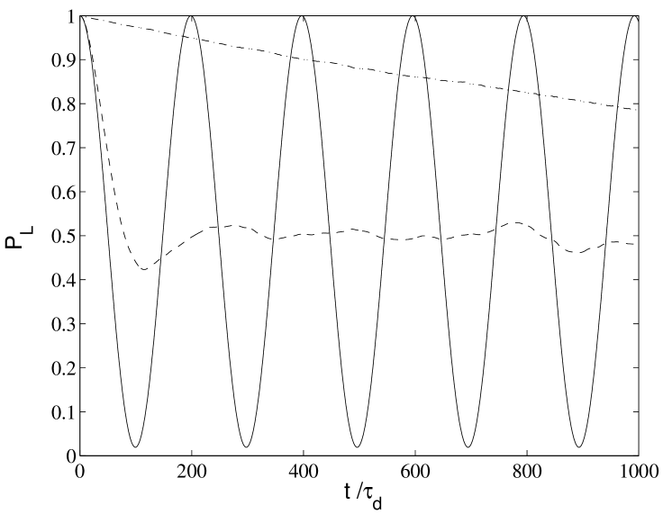
Figure 1: Fig. 1, J. Grondalski, Phys. Rev. E

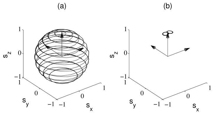
Figure 2: Fig. 2, J. Grondalski, Phys. Rev. E

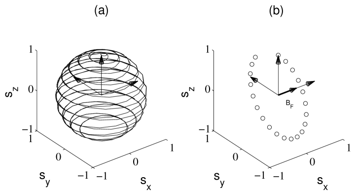
Figure 3: Fig. 3, J. Grondalski, Phys. Rev. E

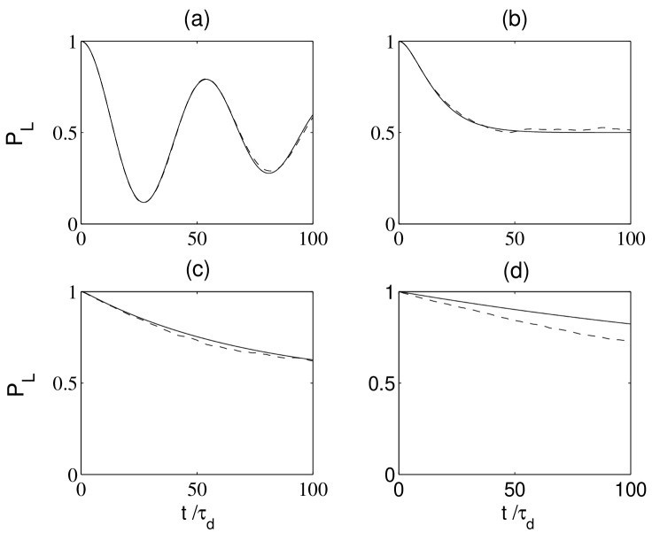
Figure 4: Fig. 4, J. Grondalski, Phys. Rev. E