Generation of eigenstates using the phase-estimation algorithm

Abstract

The phase estimation algorithm is so named because it allows the estimation of the eigenvalues associated with an operator. However it has been proposed that the algorithm can also be used to generate eigenstates. Here we extend this proposal for small quantum systems, identifying the conditions under which the phase estimation algorithm can successfully generate eigenstates. We then propose an implementation scheme based on an ion trap quantum computer. This scheme allows us to illustrate two simple examples, one in which the algorithm effectively generates eigenstates, and one in which it does not.

I Introduction

Since the inception of quantum computation Feynman (1982), people in the field have endeavored to find tasks which a quantum computer could perform more efficiently than a classical computer Deutsch and Jozsa (1992); Simon (1994); Shor (1994); Grover (1997). For a detailed introduction into the field of quantum computation and information, see Nielsen and Chuang (2000). The algorithm which has by far generated the most interest is Shor’s factoring algorithm Shor (1994), as it enables the cracking of the RSA encryption system Rivest et al. (1978). Kitaev Kitaev generalized Shor’s algorithm, showing how a quantum computer can generate an eigenvalue of an arbitrary unitary operator (in the limit of a large number of qubits, and not necessarily efficiently). Due to experimental difficulties, a large scale quantum computer (if possible), will not be attainable for a number of years. However, small-scale quantum computers are already available Sackett et al. (2000). In this paper, we show how a version of the phase estimation algorithm can be implemented on a particular ‘small-scale’ quantum computer, the ion trap quantum computer.

Given some unitary operator $U$ and an approximate eigenstate; the goal of the phase estimation algorithm Kitaev ; Cleve et al. (1998) is to obtain an eigenvalue of $U$ and leave the quantum system in the corresponding eigenstate Abrams and Lloyd (1999); Zalka (1996). To accomplish this task, we shall need two quantum systems which can be coupled together. One, we shall call the index system, the other the target system. The index system is initially prepared in the state $|0\rangle$. After performing the algorithm, the index system will store an eigenvalue of the target system operator, $U$.

Traditionally both the target and index systems have been qubit registers. In this paper the index system will remain a register of qubits, however we shall allow the target system to be an arbitrary $N$-dimensional quantum system, where $N$ may be equal to infinity. For a more generalized discussion of combining continuous and discrete quantum computation see Lloyd (2000).

In Sec. II we briefly review the phase estimation algorithm then derive the analytical results which will allow us to characterize the algorithm’s performance when using only a small number of qubits. In Sec. III we derive the Hamiltonians necessary to investigate the number and displacement operators in an ion trap, and contrast the algorithms effectiveness with respect to the two different operators.

II The Phase Estimation Algorithm

In what follows, we shall assume that our index system is a register of $m$ qubits. First, we need to be able to perform the operation $\Lambda(U)$ on our coupled system. $\Lambda(U)$ is completely described by defining its action on the standard basis states of the index system, coupled to an arbitrary target system state,

$$\Lambda(U)|j\rangle_{I}|\psi\rangle_{T} = {\mathbb{I}}_{I}\otimes{U^{j}}_{T}|j\rangle_{I}|\psi\rangle_{T}$$ (1)

$$= |j\rangle U^{j}|\psi\rangle\quad\forall\ j\in\mathbb{Z}_{M},$$

where $\mathbb{Z}_{M}=\{0,1,2,\dots,M-1\}$ and $M=2^{m}$. As in the last line of Eq. (1), we shall continue to omit the subscript notation when it is clear whether a ket or operator is referring to the target or index system. We begin the algorithm by initializing our quantum computer into the state

$$|\Psi_{0}\rangle=|0\rangle|\psi\rangle.$$ (2)

Performing a $\pi/2$ rotation of each qubit in the index register results in the state

$$|\Psi_{1}\rangle=\frac{1}{\sqrt{M}}\sum^{M-1}_{j=0}|j\rangle|\psi\rangle,$$ (3)

We now perform $\Lambda(U)$ on this state giving

$$|\Psi_{2}\rangle=\Lambda(U)|\Psi_{1}\rangle = \frac{1}{\sqrt{M}}\sum^{M-1}_{j=0}|j\rangle U^{j}|\psi\rangle.$$ (4)

The final steps in the algorithm are to perform the unitary quantum Fourier transform Coppersmith (1994) on the index register and measure this register . However, before applying this transform we shall re-write Eq. (4). First we replace $|\psi\rangle$ by it’s representation as a sum of eigenvectors of $U$,

$$|\psi\rangle=\sum_{k}c_{k}|\phi_{k}\rangle,$$ (5)

where $k$ sums over the dimensionality of the target system. Hence the state $|\Psi_{2}\rangle$ can be written as

$$|\Psi_{2}\rangle = \frac{1}{\sqrt{M}}\sum^{M-1}_{j=0}|j\rangle U^{j}\sum_{k}c_{k}|\phi_{k}\rangle.$$ (6)

We shall write the eigenvalue associated with $|\phi_{k}\rangle$ as $e^{i\phi_{k}}$. Noting that $U^{j}$ applied to each eigenvector $|\phi_{k}\rangle$ is simply $e^{ij\phi_{k}}|\phi_{k}\rangle$ and changing the order of the summations we obtain

$$|\Psi_{2}\rangle=\sum_{k}c_{k}\frac{1}{\sqrt{M}}\sum^{M-1}_{j=0}|j\rangle e^{ij\phi_{k}}|\phi_{k}\rangle.$$ (7)

Lastly, for clarity we exchange the order of the systems, and replace $\phi_{k}$ with $2\pi\omega_{k}/M$, where $\omega_{k}\in\left[0,M\right)$,

$$|\Psi_{2}\rangle = \sum_{k}c_{k}|\phi_{k}\rangle\frac{1}{\sqrt{M}}\sum^{M-1}_{j=0}e^{2\pi ij\omega_{k}/M}|j\rangle.$$ (8)

It is now not hard to show that taking the quantum Fourier transform of the index register results in the state

$$|\Psi_{3}\rangle = \sum_{k}c_{k}|\phi_{k}\rangle\sum^{M-1}_{j=0}f(\omega_{k},j)|j\rangle,$$ (9)

where

$$f(\omega_{k},j) = \left\{\begin{array}[]{c@{\ :\ }l}\frac{1}{M}\frac{\sin(\pi\omega_{k})}{\sin(\pi\frac{\omega_{k}-j}{M})}e^{\pi i(\omega_{k}-\frac{\omega_{k}-j}{M})}&\omega_{k}\not=j\\ 1&\omega_{k}=j.\end{array}\right.$$ (12)

As we will see shortly, it is helpful to note that

$$|f(\omega_{k},j)| \geq |\mathrm{sinc}(\omega_{k}-j)|,$$ (13)

for all $\omega_{k}\in\left[0,M\right)$ and $j\in\mathbb{Z}_{M}$. A plot of $|f(\omega_{k},j)|$ is shown in Fig. 1 where $M=16$ and $j$ has been set to 5.

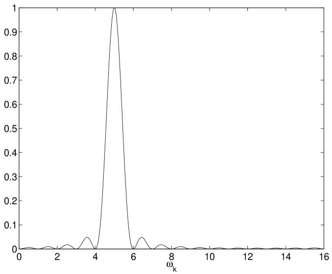
Figure 1: A plot of $|f|$ as a function of $\omega_{k}$, with $M=16$ and $j=5$.

Finally, measuring the index register will, with high probability, yield an approximate eigenvector. To understand this, let us begin by looking at the most simplified case. Suppose for a moment, that we have $\omega_{k}\in\mathbb{Z}_{M}$ for all $k$, then

$$f(\omega_{k},j) = \delta_{\omega_{k}-j}.$$ (14)

Thus Eq. (9) simplifies to

$$\sum_{k}c_{k}|\phi_{k}\rangle|\omega_{k}\rangle.$$ (15)

If we add the assumption that no two values of $k$ give the same $\omega_{k}$ (i.e. we have no degeneracy ) then upon measuring the index register, we will obtain $|\omega_{k}\rangle$, and hence $e^{i\phi_{k}}$, with probability $|c_{k}|^{2}$, and leave the target system in the eigenstate $|\phi_{k}\rangle$.

Removing the assumption of zero degeneracy, measuring the index register still allows us to obtain some eigenvalue $e^{2\pi ij/M}$, however the target system is now left in the state

$$\frac{1}{\sqrt{\mathcal{N}}}\sum_{k^{\prime}}c_{k^{\prime}}|\phi_{k^{\prime}}\rangle$$ (16)

where $k^{\prime}=\{k:\omega_{k}=j\}$, and $\mathcal{N}=\sum_{k^{\prime}}|c_{k^{\prime}}|^{2}$ is a normalization constant.

Finally, we shall remove the assumption that the $\omega_{k}$ must be elements of $\mathbb{Z}_{M}$. The probability $P(j)$, of measuring the index register in some basis state $|j\rangle$ is

$$P(j) = \sum_{k}|\langle\phi_{k}|\langle j|\Psi_{3}\rangle|^{2}$$ (17)

$$= \sum_{k}|c_{k}f(\omega_{k},j)|^{2}.$$

Having measured the index register to be in some state $|j\rangle$, the target system is left in the state

$$|\psi^{\prime}_{j}\rangle = \sum_{k}c^{\prime}_{k}|\phi_{k}\rangle,\quad c^{\prime}_{k}=\frac{c_{k}f(\omega_{k},j)}{\sqrt{\mathcal{N}}}$$ (18)

where $\mathcal{N}=\sum_{k}|c_{k}f(\omega_{k},j)|^{2}$.

In order to gain some useful information from Eqs. (17) and (18), let us assume that our initial target system state $|\psi\rangle$ is an approximate eigenstate of $|\phi_{q}\rangle$ for some $q$ such that

$$|c_{q}|^{2}\equiv|\langle\phi_{q}|\psi\rangle|^{2} = p.$$ (19)

Remembering that $\omega_{q}$ will be some real number between $0$ and $M$, we define $\lfloor\omega_{q}\rfloor$ to be the nearest $m$-bit integer less than $\omega_{q}$, and $\lceil\omega_{q}\rceil$ to be the nearest $m$-bit integer greater than $\omega_{q}$, where modulo $M$ has been assumed. The probability of measuring the index register in either the state $|\lfloor\omega_{q}\rfloor\rangle$ or $|\lceil\omega_{q}\rceil\rangle$ is

$$P(\lfloor\omega_{q}\rfloor\mathrm{or}\lceil\omega_{q}\rceil) = \sum_{k}|c_{k}f(\omega_{k},\lfloor\omega_{q}\rfloor)|^{2}$$ (20)

$$\quad+\quad\sum_{k}|c_{k}f(\omega_{k},\lceil\omega_{q}\rceil)|^{2}$$

$$\geq |c_{q}f(\omega_{q},\lfloor\omega_{q}\rfloor)|^{2}+|c_{q}f(\omega_{q},\lceil\omega_{q}\rceil)|^{2}$$

$$\geq |c_{q}|^{2}\ 2\ \mathrm{sinc}^{2}(0.5)$$

$$> 0.8p.$$

Hence, with probability greater than $0.8p$ we will obtain an approximate eigenvalue associated with $|\phi_{q}\rangle$ which differs in phase from the actual eigenvalue by less than $2\pi/2^{m}$. Thus, if $p$ is reasonably large, we have a high probability of finding the best estimate of the eigenvalue. However, as we shall see, large $p$ does not imply that we will improve on the approximate eigenstate.

Suppose we measure the index register in the state $|[\omega_{q}]\rangle$, where $[\omega_{q}]$ denotes the closest $m$-bit integer to $\omega_{q}$. (N.B. This will occur with probability greater than $0.4p$, as $|f(\omega_{q},[\omega_{q}])|^{2}>0.4$.) The key question that we wish to address in this paper is: has our initial approximate eigenstate improved? Letting $p^{\prime}\equiv|c^{\prime}_{q}|^{2}$, we are effectively asking what bounds can be placed on $p^{\prime}$? For an arbitrary $U$ it is obvious that the upper bound of $p^{\prime}=1$ can be obtained by setting $|\psi\rangle=|\phi_{q}\rangle$. We now investigate the lower bound by dividing the eigenstates into three disjoint sets,

$$\mathcal{Q} = \{q\},$$

$$\mathcal{G} = \{g:g\not=q,|\omega_{g}-[\omega_{q}]|\leq 1\}\ \mathrm{and}$$ (21)

$$\mathcal{H} = \{h:|\omega_{h}-[\omega_{q}]|>1\}.$$

We now have

$$p^{\prime} = \frac{p|f(\omega_{q},[\omega_{q}])|^{2}}{\mathcal{N}},$$ (22)

with

$$\mathcal{N} = p|f(\omega_{q},[\omega_{q}])|^{2}+\sum_{g\in\mathcal{G}}|c_{g}|^{2}|f(\omega_{g},[\omega_{q}])|^{2}$$ (23)

$$\quad+\sum_{h\in\mathcal{H}}|c_{h}|^{2}|f(\omega_{h},[\omega_{q}])|^{2}.$$

Using Eqs. (12) and (II), it is not hard to show

$$0.4< \ \ |f(\omega_{q},[\omega_{q}])|^{2}\ \ \leq 1$$

$$0\leq |f(\omega_{g},[\omega_{q}])|^{2} \leq 1$$ (24)

$$0\leq |f(\omega_{h},[\omega_{q}])|^{2} \leq\lambda$$

where $\lambda=|f(1.5,0)|^{2}$. As $m$ increases $\lambda$ tends to $(\frac{2}{3\pi})^{2}\approx 0.045$. However for our analysis it is sufficient to note that $0.045<\lambda<0.05$ for $m>3$. Eq. (II) leads to the lower bound

$$p^{\prime} \geq \frac{p|f(\omega_{q},[\omega_{q}])|^{2}}{p|f(\omega_{q},[\omega_{q}])|^{2}+(1-\lambda)G+\lambda(1-p)}$$ (25)

where $G=\sum_{g}|c_{g}|^{2}$. Fig. 2 contains a plot of this lower bound as a function of $G$ for $|f(\omega_{q},[\omega_{q}])|^{2}=0.6$ and various values of $p$. The circles indicate the points at which the minimum of $p^{\prime}$ equals $p$.

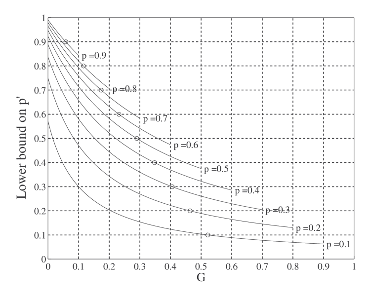
Figure 2: The lower bound on $p^{\prime}$ as a function of $G$ for $|f(\omega_{q},[\omega_{q}])|^{2}=0.6$ and various values of $p$. The circles indicate the points at which the minimum of $p^{\prime}$ equals $p$.

Thus, we see that by endeavoring to make $G$ as small as possible, we increase the amplitude of $|\phi_{q}\rangle$. For a given $U$ and $|\psi\rangle$, $G$ can be made arbitrarily small by increasing $m$. However, we are interested in the performance of the algorithm for small values of $m$. We shall now look at $G$’s dependence on $U$ and $|\psi\rangle$ by attempting to create eigenvectors for both the number and displacement operator in a ion trap.

III An Iontrap Implementation

We first derive the Hamiltonian for $\Lambda(U)$, where $U$ is the evolution operator associated with the number operator, and investigate the phase estimation algorithm’s performance for various initial states. We then derive the Hamiltonian for the more complicated case of $U$ being the displacement operator. For both of these examples the index register will be two electronic levels of $m$ ions in a linear ion trap, and the target system will be the center-of-mass (CM) vibrational mode of the ions.

III.1 The Number Operator

Consider the standard Hamiltonian of the one dimensional harmonic oscillator,

$$H=\hbar\omega(a^{\dagger}a+\frac{1}{2}).$$ (26)

where $a^{\dagger}$ and $a$ are the creation and annihilation operators. Ignoring the over-all phase contribution of the zero energy state, the unitary operator we will first be analyzing is

$$U(t)=e^{-i\omega a^{\dagger}at}.$$ (27)

In this case, $\Lambda(U)$ is given by

$$\Lambda(U) = \exp\left({\frac{-it}{\hbar}\sum_{j=0}^{m-1}H_{j}}\right),$$ (28)

where

$$H_{j} = \hbar a^{\dagger}a2^{j}\omega(\sigma_{z}^{(j)}+\frac{1}{2}).$$ (29)

The inversion operator for each ion is defined by $\sigma_{z}^{(j)}=(|0\rangle\langle 0|-|1\rangle\langle 1|)/2$. This Hamiltonian can be obtained for interaction times greater than the period of the CM vibrational mode by applying a set of far-detuned standing wave pulses to the ion D’Helon and Milburn (1996).

We begin our analysis by initializing the CM mode in some phonon number state $|n\rangle$ Meekhof et al. (1996), and setting $\omega t=2\pi(1-1/M)$. It is important to note that we are assuming that all the higher vibrational modes are in the vacuum state. Assuming no errors, applying the phase estimation algorithm results in the index register being measured in the state $|n\mod M\rangle$ and the target system is left unchanged. If we now let $\omega t$ be some arbitrary value, applying the algorithm will leave the target system unchanged, and the index system will be measured in the state $|j\rangle$ with probability

$$P(j) = \left|f\left(\frac{-\omega tnM}{2\pi},j\right)\right|^{2}$$ (30)

Let us consider the more interesting situation where the target system is initialized in some coherent state $|\alpha\rangle$. We can utilize the phase estimation algorithm to transform the state of the target system into an approximation to a Fock state.

For example, suppose we use four index qubits, $\omega t=1$ and we choose to approximate the Fock state $|n=9\rangle$ by using the coherent state $|\alpha=3\rangle$. In this example we perhaps might think that $|\alpha=3\rangle$ is not a good approximate state because $p\approx 0.13$ however the fact that $G<0.035$ indicates the algorithm should work well. Applying the algorithm and measuring the index register in the state $|9\rangle$, we obtain $p^{\prime}\approx 0.93$. The initial and final target state for this scenario is shown in Fig. 3.

Figure 3: Fock state distributions for the target system initially in a coherent state with $\alpha=3$, and the state of the system after applying the phase estimation algorithm and measuring the four index qubits.

Having shown that the phase estimation algorithm can be used to generate Fock states from coherent states, we now attempt to generate eigenstates of the displacement operator.

III.2 The Displacement Operator

The displacement operator applied to the CM vibrational mode is defined as

$$D(\alpha) = \exp(\alpha a^{\dagger}-\alpha^{*}a).$$ (31)

Thus the operator we wish to apply is

$$\Lambda(D) = \exp\left({\frac{-it}{\hbar}\sum_{j=0}^{m-1}H_{j}}\right),$$ (32)

where the $H_{j}$ are now defined as

$$H_{j} = i\hbar(\alpha a^{\dagger}-\alpha^{*}a)2^{j}(\sigma_{z}^{(j)}+\frac{1}{2}).$$ (33)

It has already been shown Monroe et al. (1996) that conditional displacement operations such as the Hamiltonian in Eq. (33) can be performed in an ion trap.

It is not hard to show that

$$D(de^{i(\phi+\frac{\pi}{2})})|\alpha,\varepsilon\rangle \approx e^{i2d|\alpha|e^{-r}}|\alpha,\varepsilon\rangle$$ (34)

for large values of squeezing parameter $r$ and where $\alpha=|\alpha|e^{i\phi}$, $\varepsilon=re^{2i\phi}$ and

$$|\alpha,\varepsilon\rangle \equiv S(\varepsilon)D(\alpha)|0\rangle$$ (35)

is a squeezed coherent state. Thus the squeezed coherent states $|\alpha,\varepsilon\rangle$ form approximate eigenvectors of the displacement operator $D(de^{i(\phi+\frac{\pi}{2})})$.

Without loss of generality we can set $\phi=0$ in which case the eigenstates of the displacement operator are simply the position eigenstates. It is then not hard to show that for small fixed $m$, $G\approx 1-p$, which leads to $p^{\prime}\approx p$. Thus applying the phase estimation algorithm to squeezed displaced states does not produce improved eigenstates of the displacement operator.

IV Conclusion

We have shown that the phase estimation algorithm can be used to generate eigenstates of the number operator, even when we severely limit the size of the index system. It would be interesting to see if an analogous implementation could be performed using cavity QED, allowing generation of photon number states with only small numbers of trapped atoms. We have also shown that the algorithm’s performance depends on the relation between the approximate eigenstate and the spectrum of the operator. We can gauge the algorithm’s performance by calculating a parameter $G$.