Observation of power-law scaling for phase transitions in linear trapped ion crystals

Abstract

We report an experimental confirmation of the power-law relationship between the critical anisotropy parameter and ion number for the linear-to-zigzag phase transition in an ionic crystal. Our experiment uses laser cooled calcium ions confined in a linear radio-frequency trap. Measurements for up to 10 ions are in good agreement with theoretical and numeric predictions. Implications on an upper limit to the size of data registers in ion trap quantum computers are discussed.

Ions confined in linear radio-frequency traps, and cooled by laser radiation, will condense into a crystalline state. Such crystals are the most rarefied form of condensed matter known [1]. Besides being of inherent scientific interest for this reason, cold trapped ions have a growing number of applications, notably spectroscopy [2, 3, 4], frequency standards [3, 5], and quantum computing [6, 7]. The existence of different kinds of phase transitions of these crystals has been known for some time [8, 9] and has been the subject of various theoretical and numeric studies [10, 1, 11]. Previous experimental work identified different crystal phases/configurations in a quadrupole ring trap [9]. Here we explicitly investigate the $\it{transition}$ between two of these phases: the linear and the zigzag configurations. We report the first experimental confirmation of one of the key theoretical/numeric predictions for the linear-to-zigzag transition, namely the existence of a power-law relating the critical anisotropy parameter to the number of ions in the crystal. Further, we discuss the usefulness of this power-law expression in determining the ultimate size of a quantum logic register realizable using a single ion trap.

The potential energy of a crystal of $N$ identical ions of mass $M$ and charge $e$ confined in an effective three-dimensional harmonic potential is

$$U\left({\bf r}_{1},{\bf r}_{2},\ldots{\bf r}_{N}\right) = \frac{M(2\pi)^{2}}{2}\sum_{n=1}^{N}\left(\nu_{x}^{2}x_{n}^{2}+\nu_{y}^{2}y_{n}^{2}+\nu_{z}^{2}z_{n}^{2}\right)$$ (2)

$$+\frac{e^{2}}{8\pi\epsilon_{0}}\sum_{\stackrel{{\scriptstyle\scriptstyle n,m=1}}{{m\neq n}}}^{N}\frac{1}{|{\bf r}_{n}-{\bf r}_{m}|}\ ,$$

where ${\bf r}_{n}=\left(x_{n},y_{n},z_{n}\right)$ is the postion vector of the $n-th$ ion, and $\nu_{x}$, $\nu_{y}$ and $\nu_{z}$ are the trapping potential frequencies in the three directions. Assume the trapping potentials are approximately equal in the two transverse directions ($x$ and $y$), so that $\nu_{x}\approx\nu_{y}\approx\nu_{r}$, and the trapping potential in the axial ($z$) direction is different than in the other two directions. This anisotropy is characterized by the parameter $\alpha=(\nu_{z}/\nu_{r})^{2}$. Work by Schiffer [1] and Dubin [11] predicts that the ions undergo a phase transition from a linear to a zigzag configuration at a critical anisotropy value $\alpha_{crit}$. The predicted power-law scaling for $\alpha_{crit}$ versus the number of trapped ions $N$ is:

$$\alpha_{crit}=cN^{\beta},$$ (3)

where the constants found empirically by Schiffer are $c=2.53$ and $\beta=-1.73$ [12]. Later in this paper we provide a simple alternative approach which produces qualitative agreement with Schiffer’s results but is based on a stability analysis of the transverse oscillatory modes, rather than on numerical simulations of the equilibrium crystalline configurations.

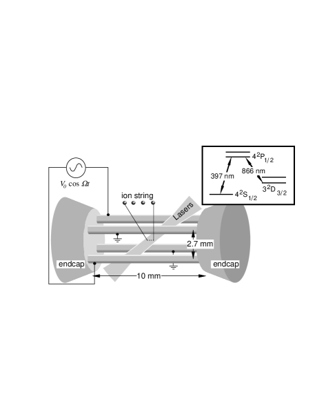
FIG. 1.: Trap electrodes include four 1-mm diameter rods and two endcaps. Rf trapping voltages $V_{0}$ range from 60-200 V, producing radial frequencies $\nu_{r}=200-700$ kHz. Endcap voltages range from 10-200 V, producing axial frequencies $\nu_{z}=80-390$ kHz. Outer support rods (not shown) double as compensation electrodes for moving ions radially within the trap. The insert shows a level diagram for ⁴⁰Ca⁺.

We studied the zigzag phase transition using strings of ⁴⁰Ca⁺ ions confined in a linear radio-frequency quadrupole trap. Trap electrodes (see Fig. 1 or Ref. [13]) consist of four rods and two conical endcaps. An rf drive at $\Omega/2\pi=6$ MHz is applied to two diagonally opposite rods to produce a radial confining pseudo-potential [14] with frequency $\nu_{r}$ proportional to the rf trapping voltage $V_{0}$ (for example, [15]). Axial confinement is provided by a static potential applied to the two endcap electrodes, resulting in a harmonic potential with frequency $\nu_{z}$ proportional to the square root of the endcap voltage. Anharmonic contributions to the axial potential energy are estimated to be less than $3\times 10^{-7}$ the harmonic contribution, and are thus ignored.

Calcium ions are introduced into the trap by intersecting an atomic beam with an electron beam. Laser cooling on the S_1/2 to P_1/2 transition at 397 nm (see Fig. 1) cools the ions so that a crystallized string is formed along the trap axis. The resulting 397 nm ion fluorescence is detected in the horizontal plane along a direction perpendicular to the trap axis by both a CCD camera and a photomultiplier tube. An 866 nm laser returns ions falling into the D_3/2 metastable state to the cooling cycle. The 397 nm light is produced by doubling 794 nm diode-laser light which is intensified by a tapered amplifier; the 866 nm beam is also produced by a diode laser.

For each measurement of $\alpha_{crit}$, the rf trapping potential is lowered, keeping the endcap voltage constant, until the transition to a zigzag pattern is observed. The rf potential is then repeatedly raised and lowered to determine the reproduceability of the transition point and to rule out hysteresis. At the identified critical rf voltage, we measure the radial and axial resonant frequencies. The measurements are repeated for a range of endcap voltages and then for different numbers of ions $N$.

To determine the rf trapping voltage at which the linear crystal becomes zigzag, the voltage is lowered until the equilibrium position of at least one of the ions moves visibly (0.5-1.5 pixels $\approx 0.3-1.0$ $\mu$m) on the CCD camera image. Axial shifts are detected more easily than radial shifts; therefore, movement in the axial direction is used as the diagnostic to identify the phase transition. Moreover, observations show the spacing between the two innermost ions to be most sensitive to this axial reorganization. The critical rf voltage is determined to within $\pm$0.1 V out of 3-8 V on the synthesizer generating the rf trapping voltage. This 0.1 V resolution, corresponding to 8-16 kHz uncertainty in radial frequency, is limited by the voltage change necessary to move an ion visibly on the CCD camera rather than by the synthesizer itself.

The radial and axial frequencies are individually measured by applying an external drive and observing melting of the crystal into a diffuse but still stable cloud when the drive frequency is resonant. Note that although the ions are driven at a center-of-mass frequency, coupling to higher order modes heats the string until it melts. The external drive is the output of a function generator, attenuated and capacitively coupled through 1000 pF to one endcap electrode. Resonant frequencies are measured reproduceably to within $\pm$1-2 kHz by stepping repeatedly back and forth through the typical 1-4 kHz range in which melting is observed. Since the azimuthal symmetry of the trap is not perfect, we measure two separate radial frequencies, differing from each other by 1-2$\%$. The data presented includes only the smaller radial frequency (corresponding to the weaker axis of the radial well) which is responsible for the zigzag instability onset.

Figure 2 shows the radial versus axial frequencies at which the linear-to-zigzag phase transition was observed for string lengths up to $N=10$. Figure 3 shows the average $\alpha_{crit}$ as a function of $N$, and demonstrates the predicted scaling behavior for these critical parameters. In both figures, the solid lines are results from our theoretical analysis (presented below) with no free parameters. Although the measurements of $\alpha_{crit}$ lie slightly above theory, the overall agreement within the 5-6$\%$ error bars is quite remarkable for a second order phase transition.

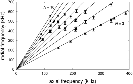
FIG. 2.: Measured radial versus axial frequencies (points), at the onset of the zigzag instability, agree well with the prediction of our theoretical analysis (lines). Measurements were taken on seven different days, with some days dedicated to a particular length ion string and other days spent studying up to six different length strings. Theory lines pass through the origin and have slopes $\nu_{r}/\nu_{z}=(\alpha_{crit})^{-1/2}$, increasing with ion number for $N=3$ (minimum slope shown) through $N=10$ (maximum slope shown). Error bars (see text) are dominated by the uncertainty in determining the critical rf voltage for zigzag onset while the axial frequency is held fixed.

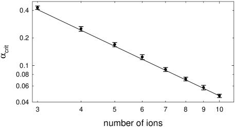
FIG. 3.: Measured values (points) of the critical anisotropy parameter $\alpha_{crit}$ versus ion number $N$ agree well with a fit to the predictions of our theoretical analysis (line). Each point is a weighted average of measured values from Fig. 2, as is each error bar.

In Fig. 2, vertical error bars are dominated by the 8-16 kHz resolution in determining the onset of the zigzag mode as described above, but also include (in quadrature) the 1-2 kHz measurement resolution of the radial frequency. Horizontal errors representing the axial frequency measurement resolution are smaller than the point size and not shown, but are included when calculating the error for a measured $\alpha_{crit}$. In Fig. 3, each plotted value is a weighted average of measured $\alpha_{crit}$’s. Corresponding error bars are taken to be weighted average errors rather than quadrature sums of the individual $\alpha_{crit}$ errors, because they represent detection resolution rather than statistical errors and performing many measurements would not be expected to reduce their size.

An unaccounted source of error arises from the threshold axial shift of 0.5-1.5 pixels required to detect a phase transition. Any smaller axial shifts due to onset of the zigzag mode at higher rf voltages go undetected. Investigations tracking the axial position of an ion near the center of a linear crystal as a function of rf trapping voltage were performed to estimate the size of this detection threshold error. Examples such as those shown in Fig. 4 reveal that once a phase transition is detected, the axial equilibrium moves roughly linearly with rf voltage at a rate of 0.3-1.1 pixels per 0.1 V step of the drive synthesizer. Not surprisingly, the weaker trap settings – low endcap voltage and small ion number – produce the larger amount of movement per voltage step but also require the larger threshold shift. Underestimates in the critical trapping voltage due to this effect, therefore, end up of the same order as the 0.1 V resolution error already assigned. This detection threshold error accounts in part for the slightly high trend exhibited by the measured $\alpha_{crit}$’s. Alternatively, ignoring the detection threshold error, our measurement can instead be interpreted as an upper bound on $\alpha_{crit}$.

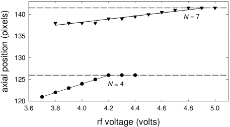
FIG. 4.: Axial position as a function of rf voltage for an ion nearest to, but not at the center of, a 4 ion string (circles) and a 7 ion string (triangles). Dashed lines show the steady state axial position for high rf voltages. Solid lines are fits to the points whose rf voltages lie at or below the critical value.

Trapping and cooling parameters were varied outside their normal ranges to rule out systematic effects. Detuning the 397 nm laser as far as possible to longer or shorter wavelengths, while still maintaining crystallization, altered neither the measured resonant frequencies nor the measured critical rf voltage. Similar tests involving the 866 nm laser wavelength showed no effects. Finally, for each new endcap voltage, care was taken to move the ion string to the radial center of the rf quadrupole potential. Ions not centered in this potential experience micromotion at the 6 MHz trap frequency. This driven motion, detected as a modulation on the ion fluorescence intensity, was used as a diagnostic to find the optimal position along one radial direction [15]. The diagnostic of micromotion for the orthogonal radial direction was the observation of a radial shift in ion position upon weakening or strengthening the pseudo-potential well, because an ion’s position in the pseudo-potential will depend on the potential well strength unless the ion is centered [15]. Ions were moved radially by applying voltages to the compensation electrodes, which were typically tuned to $\pm$1 V; tests detuning them by 5-10 V revealed no change in measured resonant frequencies or in critical rf voltages.

We now present a simple theoretical analysis of the onset of zigzag instability. The equilibrium positions of the ions are determined by the condition that the potential be a minimum, i.e. $\nabla_{n}U=0\,(n=1,\ldots N)$. For the case of strong anisotropy ($\alpha\ll 1$), the ions are configured along a line in the $z$-direction. The solutions to the equilibrium equations in this case have been investigated by various authors (see, for example [16, 17, 18]); we denote the equilibrium position of the $n-th$ ion by ${\bar{\bf r}}_{n}=\left(0,0,{\bar{z}}_{n}\right)$.

Small oscillations of the ions about their equilibrium positions are described by the Lagrangian [17, 19]

$$L = \frac{M}{2}\left[\sum_{n=1}^{N}\dot{\zeta}^{2}_{n}-\omega^{2}_{z}\sum_{n,m=1}^{N}A_{n,m}\zeta_{n}\zeta_{m}\right]$$ (4)

$$+ \frac{M}{2}\left[\sum_{n=1}^{N}\dot{\xi}^{2}_{n}-\omega^{2}_{x}\sum_{n,m=1}^{N}B_{n,m}\xi_{n}\xi_{m}\right]$$ (5)

$$+ \frac{M}{2}\left[\sum_{n=1}^{N}\dot{\eta}^{2}_{n}-\omega^{2}_{y}\sum_{n,m=1}^{N}B_{n,m}\eta_{n}\eta_{m}\right]\ ,$$ (6)

where $(\xi_{n},\eta_{n},\zeta_{n})$ are the displacements of the $n-th$ ion from its equilibrium position in the $(x,y,z)$ directions, respectively. The coupling matrices $A_{n,m}$ and $B_{n,m}$ are given by the formulae (following Ref. [17])

$$A_{n,m} = \left\{\begin{array}[]{ll}1+2{\displaystyle\sum^{N}_{\stackrel{{\scriptstyle\scriptstyle p=1}}{{p\neq m}}}\frac{\ell^{3}}{\left|{\bar{z}}_{m}-{\bar{z}}_{p}\right|^{3}}}&{\rm if}\quad n=m,\\ \rule{0.0pt}{21.52771pt}{\displaystyle\frac{-2\ell^{3}}{\left|{\bar{z}}_{m}-{\bar{z}}_{n}\right|^{3}}}&{\rm if}\quad n\neq m.\end{array}\right.$$ (9)

$$B_{n,m} = \left(\frac{1}{\alpha}+\frac{1}{2}\right)\delta_{n,m}-\frac{1}{2}A_{n,m}\ ,$$ (10)

where $\ell=\left[e^{2}/4\pi\epsilon_{0}M(2\pi\nu_{z})^{2}\right]^{1/3}$ is a length scale and $\delta_{n,m}$ is the Kronecker delta.

The eigenvectors and eigenvalues of the real, symmetric, positive-definite matrix $A_{n,m}$ define the normal modes of oscillation of the ions along the $z$-direction. Because of their importance to quantum computing, they have been studied in some detail [17, 19]. The eigenvectors are defined by the formula $\sum_{m=1}^{N}A_{n,m}b^{(p)}_{m}=\mu_{p}b^{(p)}_{n}$, where $\mu_{p}>0$ is the eigenvalue, $b^{(p)}_{n}$ the normalized eigenvector, and $p$ $(=1,\ldots N)$ the mode index (the modes being enumerated in order of increasing eigenvalue).

From the definition of the coupling matrix for the radial oscillations, $B_{n,m}$, we see that it has identical eigenvectors to $A_{n,m}$, but has different eigenvalues:

$$\sum_{m=1}^{N}B_{n,m}b^{(p)}_{m}=\left(\frac{1}{\alpha}+\frac{1}{2}-\frac{\mu_{p}}{2}\right)b^{(p)}_{n}.$$ (11)

For these oscillations, the eigenvalues are no longer always positive. Indeed, as $\alpha$ is increased, a critical value occurs for which one of the eigenvalues of the radial oscillations becomes zero. Beyond this point the radial oscillation is unstable and so is the linear configuration: this marks the onset of the zigzag mode. The critical value of $\alpha$ for which this occurs is given by the exact result $\alpha_{crit}(N)=2/(\mu_{N}-1)$, where $\mu_{N}$ is the largest eigenvalue of the matrix $A_{n,m}$ for a given number of ions $N$. The value of $\mu_{N}$ in general must be determined by numerically diagonalizing the matrix $A_{n,m}$ for each value of $N$, but the expression for $\alpha_{crit}(N)$ is exact.

We can approximate $\alpha_{crit}(N)$ as the power-law in Eq. 3 in order to compare it to our experimental measurements. Table I compares the constants $c$ and $\beta$ (see Eq. 3) derived from the measurements, from a fit to our theory (over $N=3-10$), and from Schiffer’s fit. We emphasize that no matter how well any model calculates $\alpha_{crit}$ for a specific $N$, the power-law deduced for $\alpha_{crit}$ versus $N$ is still approximate and must be obtained from a fit of many calculated $\alpha_{crit}$’s. In light of this, the three sets of coefficients are close, particularly for $\beta$. Small discrepancies may be explained by the fact that the exact expression for $\alpha_{crit}(N)$ is $\it{not}$ a power-law, and that Schiffer’s predicted values were deduced from a fit of 10 $\alpha_{crit}$ values over the range $N=2-500$ whereas we fit over just the experimental range $N=3-10$. Fitting, instead, over all values in the range $N=2-100$, yields the constants $c=2.88\pm 0.03$ and $\beta=-1.773\pm 0.003$, which are more appropriate (as are Schiffer’s) for large $N$ applications of the power-law discussed below.

TABLE I.: Scaling constants $c$ and $\beta$ from fits of the experimental and theoretical data shown in Fig. 3 and from Schiffer’s numerical results. Standard errors from our linear regressions are included. (The error in Schiffer’s linear regression was not reported). An additional $-5\%$ experimental uncertainty in $\alpha_{crit}$ is included to account for the detection threshold error discussed earlier; it dominates the $-0.2$ uncertainty in $c$ and the $\pm 0.04$ uncertainty in $\beta$.

	Experiment	Our Theory	Schiffer’s Results
$c$	$3.23^{+0.06}_{-0.2}$	$2.94\pm 0.07$	2.53
$\beta$	$-1.83\pm 0.04$	$-1.80\pm 0.01$	-1.73

Using the power-law expression, we illustrate how to estimate the maximum number of ions it is reasonable to confine along the trap axis. This gives one possible upper limit to the size of data registers for quantum computation with on-axis ions in a linear trap. Rewriting Eq. 3 gives an upper limit $N_{crit}$ to the number of ions one can trap in the linear configuration: $N_{crit}=(\nu_{z}/\sqrt{c}\nu_{r})^{2/\beta}$. Experimental limitations will dictate how large the ratio $\nu_{z}/\nu_{r}$ can be made, but this expression should prove useful in optimizing future designs of ion traps.

In summary, a simple theoretical analysis has produced the critical anisotropy parameter $\alpha_{crit}$ for the linear-to-zigzag phase transition. Experimental measurements have provided a confirmation of the predicted power-law scaling for $\alpha_{crit}$ versus $N$ which had until now been untested. From this scaling we obtain an expression for an upper limit to the size of linear data registers for quantum computation in these traps.

We are grateful to D. J. Berkeland and A. G. Petschek for helpful conversations. This work was supported by the National Security Agency.

REFERENCES

- [1] J. P. Schiffer, Phys. Rev. Lett. 70, 818 (1993).
- [2] M. Roberts et al., Phys. Rev. Lett. 78, 1876 (1997).
- [3] D. J. Berkeland et al., Phys. Rev. Lett. 80, 2089 (1998).
- [4] R. G. DeVoe and R. G. Brewer, Phys. Rev. Lett. 76, 2049 (1996).
- [5] P. T. H. Fisk, Rep. Prog. Phys. 60, 761 (1997).
- [6] J. I. Cirac and P. Zoller, Phys. Rev. Lett. 74, 4091 (1995).
- [7] C. A. Sackett et al., Nature 404, 256 (2000).
- [8] D. J. Wineland et al., Phys. Rev. Lett. 59, 2935 (1987).
- [9] G. Birkl, S. Kassner, and H. Walther, Nature 357, 310 (1992).
- [10] R. W. Hasse and J. P. Schiffer, Ann. Phys. 203, 419 (1990).
- [11] D. H. E. Dubin, Phys. Rev. Lett. 71, 2753 (1993).
- [12] The printed values of the parameter in [1] appear to be misprinted as the reciprocals of their true values.
- [13] R. J. Hughes et al., Fortschr. Phys. 46, 329 (1998).
- [14] P. H. Dawson, Quadrupole Mass Spectrometry and Its Applications (Elsevier Scientific Publishing Company, New York, 1976).
- [15] D. J. Berkeland et al., J. Appl. Phys. 83, 5025 (1998).
- [16] A. Steane, Appl. Phys. B 64, 623 (1997).
- [17] D. F. V. James, Appl. Phys. B 66, 181 (1998).
- [18] T. P. Meyrath and D. F. V. James, Phys. Lett. A 240, 37 (1998).
- [19] D. Kielpinski et al., Phys. Rev. A 61, 032310 (2000).