Quantum copying can increase the practically available information

Abstract

While it is known that copying a quantum system does not increase the amount of information obtainable about the originals, it may increase the amount available in practice, when one is restricted to imperfect measurements. We present a detection scheme which using imperfect detectors, and possibly noisy quantum copying machines (that entangle the copies), allows one to extract more information from an incoming signal, than with the imperfect detectors alone. The case of single-photon detection with noisy, inefficient detectors and copiers (single controlled-NOT gates in this case) is investigated in detail. The improvement in distinguishability between a photon and vacuum is found to occur for a wide range of parameters, and to be quite robust to random noise. The properties that a quantum copying device must have to be useful in this scheme are investigated.

I Introduction

It is well known that making copies of a quantum system (e.g. with a quantum copier) does not increase the amount of information present about the original. To put it another way, spreading information about the original system onto several systems does not increase the amount of information that one can obtain about the original (in fact, this usually decreases it due to noise). However, in discussions on this matter it is usually tacitly assumed that one has access to optimal measuring devices.

In practical situations, however, this is never the case. One is always restricted to imperfect measurements, due to inefficient detectors, and various sources of random noise. Although, in theory, Quantum mechanics allows one to perfectly distinguish between orthogonal states by making appropriate measurements, in practice distinguishing perfectly every time is impossible. Of course, in many situations these imperfections of measurement are insignificant, but in this article we consider those cases where such inefficiencies are relevant.

Let us investigate what can be done in principle if one is restricted to using inefficient and noisy detectors. In many practical situations what one is interested in is to determine in which one of several possible orthogonal states a system is residing. For example, this is what one does to extract transmitted information from a signal.

The basic idea explored in this article can be expressed as follows: If we can get a second chance to use the detectors at our disposal on the same state, we might do better at distinguishing it from among the range of possibilities. We will investigate what happens when one makes copies of the original state. If the available detectors are fairly poor, then one may hope that making even imperfect copies may still give improvements if one can then make independent measurements on each of the copies.

Copying machines in general use two approaches. One of the extreme cases is a classical copying machine, where measurements (destructive or non-destructive) are made on the original state, the results of which are then fed as parameters into some state preparation scheme that attempts to construct a copy of the original. This approach obviously allows one to generate an arbitrary amount of copies, possibly all identical to each other. The opposite extreme is a fully quantum copying machine that by some process that is unseen by external observers (a “black box”), creates a fixed number of copies, usually destroying the original in the process. Naturally in a realistic situation, noise will additionally degrade the quality of the copies, and copiers that utilize both of the processes above are obviously also possible.

Since one’s detection resources are restricted to imperfect detectors that discard some information about the state, then it becomes immediately obvious that classical copying gains you nothing. Any information about the original state that you can extract from the copies can be extracted just as well from the measurement results used to produce the copies – and these are made with those imperfect detectors. Quantum copying, however, is able to give improvements, even when degraded by noise and inefficiencies, as will be seen below.

For simplicity, and because the aim is above all to demonstrate the principle at work here, we will consider situations where one wishes to distinguish between two orthogonal possibilities for the input state. Some examples of this would be single-photon detection, distinguishing spins of spin-half particles, single-photon polarization, or distinguishing between some number of photons and no photons.

This paper sets out in more detail, and expands on a previous short article dealing with this topic by the same authors[2]. Sec. II puts forward the general detection scheme that, utilizing entangling quantum copiers and inefficient detectors, allows one (if the copiers are good enough) to achieve surer detection than with the detectors alone. An example is given with a very simplified case of single-photon detection. Sec. III Develops a more realistic schematic model of single-photon detection, using a single controlled-NOT gate as the copier.

Subsequently, in Sec. IV we consider the noiseless case and analyze its performance with respect to the standard one-detector setup. We first consider the situation where one uses the measurement results to make a decision about what the original state was – the probability of being correct is compared between detection schemes. Secondly, we compare the total information about the original state that is in principle extractable from the measurement outcomes. Sec. V Looks at how robust the copier-enhanced detection scheme is to random noise in the copiers and detectors. Finally, in Sec. VI the properties that a quantum copying device must have to be useful are found.

II A Detection Scheme with Quantum Copiers

Consider the case where one of a set of possible input states are to be distinguished by a measurement scheme, using (some number of identical) imperfect detectors. That is, whether the input states are mutually orthogonal, or not, the detectors at one’s disposal do not always distinguish between the inputs with certainty. One also has some (identical) quantum copiers that can act on the possible input states. For a first look at the situation, let us suppose that the possible input states are mutually orthogonal, and that one has somehow acquired perfect quantum copiers for this set of states. Assume the copiers destroy the original, and produce two copies for simplicity. Then, an obvious way to take advantage of the copiers is to send the originals through a quantum copier, before trying to detect both copies separately. (As in Fig. 1). This basically gives one a second chance to distinguish the input state, if the detection at the first copy fails.

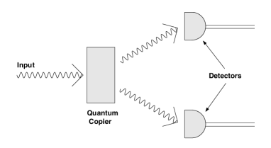
FIG. 1.: Basic detection scheme using imperfect detectors, and a quantum copier

In practice, one can never be certain whether the result given by a detector is due to noise, or the input state, but in this case, having two tries at detection allows one to better estimate whether the result was trustworthy - once again on average increasing one’s knowledge of the original.

To be slightly more concrete, consider a very simplified model of photodetection using this measurement scheme. (A more realistic model is developed in Sec. III). Suppose one has perfect copiers, and noiseless photodetectors of efficiency $\eta$. That is, the probability of a a count on the detector is $\eta$ if a photon is incident, and $0$ otherwise.

With the copier set up as in Fig. 1, if any of the detectors register a count, one can with certainty conclude that a photon was incident. So, if a photon is incident, the probability of finding it is

$$P^{(1)}_{\text{count}|\text{photon}}=\eta+(1-\eta)\eta,$$ (1)

as opposed to just $\eta$ with no copier, because one gets a “second chance” at detection. On the other hand, if no count is registered, then the probability that no photon was incident is

$$P^{(1)}_{\text{nophoton}|\text{nocount}}=\frac{1-p}{1-\eta p(2-\eta)},$$ (2)

where $p$ is the probability that a photon is incident on average, irrespective of the measurement result. The expression of Eq. (2) is always greater than $(1-p)/(1-\eta p)$, which is the probability if no copier is used. This increase reflects the added confidence that comes from both detectors failing to register the photon.

With more copiers, one can do better. Instead of placing photodetectors at the outputs of the first copier, place copiers instead , and detect photons only when they have come out of the second lot of copiers. One can continue putting in more copiers in a similar fashion. If we let the number of copiers that photons must pass through before being detected be $N$, ($N=1$ in the case considered previously) then one finds that for this simplified scheme

$$P^{(N)}_{\text{count}|\text{photon}} = 1-(1-\eta)^{(2^{N})},$$ (4)

$$P^{(N)}x_{\text{nophoton}|\text{nocount}} = \frac{1-p}{1-p+p(1-\eta)^{(2^{N})}}.$$ (5)

So as $N$ increases, the probability of detecting a photon that is present (given that it is present) approaches one. Also, the probability that no photon was present if it was not detected also approaches one.

Note that using quantum copiers, and not classical ones is vital. A classical copier would have to rely on the same imperfect photodetectors, and would actually reduce the detection efficiency, since to detect a photon at one of the two copy detectors, one must have been first detected at the copier. This gives $P^{(1)}_{\text{count}|\text{photon}}=\eta^{2}(2-\eta)$, which is always less than or equal to $\eta$ ($P^{(0)}_{\text{count}|\text{photon}}=\eta$ is achieved without any copiers at all).

III A Model of Improved Single-Photon Detection

Detection with the help of perfect quantum copiers, as briefly discussed in the previous section, is all very well, but what happens when the equipment used is noisy, and not 100% efficient? Consider the following, more realistic, model of photodetection, using the scheme outlined in Sec. II.

The possible states that are to be distinguished are the vacuum $\left|{0}\right\rangle$ and single photon $\left|{1}\right\rangle$ states. The a priori probability that the input state is a photon is $p$.

A generalized measurement on some state ${\hat{\rho}}$ can be modeled by a positive operator-valued measure (POVM) $\hat{\{}{}{A}_{i}\}$ [5, 6] described by a set of $n$ positive operators $\hat{A}{}_{i}$, such that $\sum_{i=1}^{n}\hat{A}{}_{i}=\hat{I}{}$, where $\hat{I}{}$ is the identity matrix in the Hilbert space of $\hat{\rho}{}$ (and of the $\hat{A}{}_{i}$). The probability of obtaining the $i$th result, by measuring on a state $\hat{\rho}{}$ is then

$$P_{i}=\mbox{Tr}\left[{\hat{\rho}{}\hat{A}{}_{i}}\right].$$ (6)

Now suppose the photodetectors at one’s disposal are noisy and have quantum efficiency $\eta$. The effect of these can be modeled by the POVM

$$\hat{A}{}_{+}= \eta\left|{1}\right\rangle\left\langle{1}\right|+\eta\xi\left|{0}\right\rangle\left\langle{0}\right|,$$ (8)

$$\hat{A}{}_{-}= (1-\eta)\left|{1}\right\rangle\left\langle{1}\right|+(1-\eta\xi)\left|{0}\right\rangle\left\langle{0}\right|,$$ (9)

where the operator $\hat{A}{}_{+}$ represents a count, and the operator $\hat{A}{}_{-}$ the lack of one. The parameter $\xi\in[0,1)$ controls the amount of noise. That is, $\xi\eta$ is the probability that the photodetector registers a spurious (“dark”) count when no photon is incident.

Model the quantum copier as one that has a probability $\varepsilon$ of working correctly and producing perfect copies. Otherwise, the parameter $\mu\in[-1,1]$ determines (in a somewhat arbitrary way) what is produced. This can be written

$$\hat{\rho}{}_{1}=\left|{{1}}\right\rangle\!\!\left|{{d}}\right\rangle\left\langle{{1}}\right|\!\!\left\langle{{d}}\right| \to\varepsilon\left|{{1}}\right\rangle\!\!\left|{{1}}\right\rangle\left\langle{{1}}\right|\!\!\left\langle{{1}}\right|+(1-\varepsilon)\hat{\rho}{}_{N}=\hat{\rho}{}^{1}_{1},$$ (11)

$$\hat{\rho}{}_{0}=\left|{{0}}\right\rangle\!\!\left|{{d}}\right\rangle\left\langle{{0}}\right|\!\!\left\langle{{d}}\right| \to\varepsilon\left|{{0}}\right\rangle\!\!\left|{{0}}\right\rangle\left\langle{{0}}\right|\!\!\left\langle{{0}}\right|+(1-\varepsilon)\hat{\rho}{}_{N}=\hat{\rho}{}^{1}_{0}.$$ (12)

$\left|{d}\right\rangle$ is a dummy state, that is fed into the copier, and becomes the second copy. It is included here to preserve unitarity in the perfect copying case $\varepsilon=1$. The state produced upon failure of the copier, $\hat{\rho}{}_{N}$ is independent of the original, and is given by

$$\hat{\rho}{}_{N}=(1-|\mu|)\frac{\hat{I}{}}{4}+\ \left\{\begin{array}[]{cll}\mu&\left|{{1}}\right\rangle\!\!\left|{{1}}\right\rangle\left\langle{{1}}\right|\!\!\left\langle{{1}}\right|&\text{ if }\mu>0\\ |\mu|&\left|{{0}}\right\rangle\!\!\left|{{0}}\right\rangle\left\langle{{0}}\right|\!\!\left\langle{{0}}\right|&\text{ if }\mu\leq 0\end{array}\right..$$ (13)

Here, $\hat{I}{}/4$ is the totally random mixed state. So, for $\mu=0$ a totally random noise state is produced upon failure to copy, for $\mu=-1$ vacuum, for $\mu=1$ photons in both copies, and for intermediate values of $\mu$ a linear combination of the three cases mentioned. The case briefly considered in the previous section had the parameters $\varepsilon=1$, $\xi=0$.

This model (Eq. (III)) of the copier is an extension (to allow for inefficiencies) of the Wootters-Zurek copier, which has been extensively studied [3, 7]. In the ideal case ($\varepsilon=1$), with the dummy input state in the vacuum ($\left|{d}\right\rangle=\left|{0}\right\rangle$), the transformation is:

$$\left|{{0}}\right\rangle\!\!\left|{{0}}\right\rangle\to\left|{{0}}\right\rangle\!\!\left|{{0}}\right\rangle\qquad\left|{{1}}\right\rangle\!\!\left|{{0}}\right\rangle\to\left|{{1}}\right\rangle\!\!\left|{{1}}\right\rangle.$$ (14)

This transformation can be implemented by the simplest of all quantum logic circuits, the single controlled-NOT gate. These have recently begun to be implemented for some systems (although admittedly not for single-photon systems), and are the subject of intense ongoing research, because of their application to quantum computing. This means that similar schemes to the one considered here may become experimentally realizable in the foreseeable future.

Note that the transformation (14) can be also considered an “entangler” rather than a copier. Consider its effect on the photon-vacuum superposition state

$$\frac{1}{\sqrt{2}}(\left|{0}\right\rangle+\left|{1}\right\rangle)\to\frac{1}{\sqrt{2}}(\left|{{0}}\right\rangle\!\!\left|{{0}}\right\rangle+\left|{{1}}\right\rangle\!\!\left|{{1}}\right\rangle).$$ (15)

This correlation between the copies is an essential property for the detection scheme presented here to be useful — otherwise one could not combine the results of the different detector measurements to better infer properties of the original. For example the universal quantum copying machine (UQCM)[7], which reproduces an arbitrary qubit with the best possible fidelity cannot give gains in detector efficiency via the scheme presented above, even when no random noise is added in the copying process (analogous to $\varepsilon=1$). This matter will be further investigated in Sec. VI where the properties of the copying machine required for this scheme to work are investigated.

IV The Performance of the Copier-Enhanced Scheme With Noiseless Copiers

Firstly, consider the optimum case (for the copier-enhanced detection scheme) when $\mu=-1$. In this situation, the copier produces a vacuum when it fails to work, and any noise present will come only from the possibility of dark counts by the detectors. The effect of copier noise will be considered in the next section, but for now we will ignore it, to show the general features of this setup with greater clarity.

The detection scheme outlined in Sec. III provides the observer who has the detectors with $2^{N}$ measurement results, each of which can either be a “count” (henceforth labeled as $+$), or “no count” (labeled as $-$). There are obviously better and worse ways for the observer to use these $2^{(2^{N})}$ distinct possible outcomes to distinguish between a photon or vacuum input. Let us look at two of these.

A Performance comparison for correctly choosing the most likely input state

An obvious and simple way to utilize the measurement results is to use them to decide whether it is more likely that a photon or that vacuum was input. One assumes that the person using the whole setup knows the parameters $\eta,\xi,\varepsilon,\mu$. In statistical terminology, we find the maximum likelihood estimator $\hat{\theta}$ for the parameter $\theta$ which describes the input state $\left|{\theta}\right\rangle$, and so takes on either the value $0$, or $1$.

We wish to compare how well this strategy works with the copier-enhanced scheme and with the basic one-detector setup. To this end, we will compare $Q$, the probability that this “most likely” guess for the input state (i.e. that $\hat{\theta}=\theta$) is correct. For simplicity and clarity, we will restrict the analysis of this method to the usual photodetection case when dark counts are rare ($\xi\ll 1$).

Consider first the standard detector-only setup ($N=0$). The measurement outcome probabilities $P_{j|i}$ [where $P_{j|i}$ is the probability of getting measurement result $j\in\{+,-\}$, given that the incident state was the $i$th one ($i\in\{0,1\}$)] are easily found using Eqs. (6) and (III)

$$P_{+|1}=\eta, P_{-|1}=1-\eta,$$ (17)

$$P_{+|0}=\eta\xi, P_{-|0}=1-\eta\xi.$$ (18)

Now, the estimator $\hat{\theta}(j)$, given a certain measurement result $j$, can be easily calculated from these, since $\hat{\theta}(j)=i$ iff $P_{i|j}\geq 1/2$. One finds, for example, that if a count is detected, then the most likely input was a photon [$\hat{\theta}(+)=1$] only if $p>\xi/(\xi+1)$. Similarly, the other “common sense” conclusion that if no count is seen, then it is more likely that there was no input photon [$\hat{\theta}(-)=0$] occurs only if $p<(1-\eta\xi)/[2-\eta(1+\xi)]$. This is because when $p$, the probability of photon input is almost certain, then even if you don’t see it, it becomes more likely that an incoming photon wasn’t detected than that none came in at all. Let us ignore such situations when $\hat{\theta}(+)=\hat{\theta}(-)$, since then this method tells us nothing about the input state. The situation $\hat{\theta}(+)=0,\hat{\theta}(-)=1$ never occurs. We find that for useful parameters, the probability of being correct is

$$Q(0) = P_{+|1}p+P_{-|0}(1-p)$$ (19)

$$= 1-p+\eta[p-\xi(1-p)].$$ (20)

Now we want to compare to this the probability of being correct if some quantum copiers are used to help things along. Consider the setup with only one copier ($N=1$). The measurement outcome probabilities (where $P_{jk|i}$ is the probability that given the $i$th input state, the first detector gives the result $j$, and the second detector gives the result $k$), are found using Eqs. (6) - (III), remembering that $\mu=-1$.

$$P_{++|1} = \eta^{2}[\varepsilon+(1-\varepsilon)\xi^{2}],$$ (22)

$$P_{--|1} = \varepsilon(1-\eta)^{2}+(1-\varepsilon)(1-\eta\xi)^{2},$$ (23)

$$P_{+-|1}=P_{-+|1} = \varepsilon\eta(1-\eta)+(1-\varepsilon)\eta\xi(1-\eta\xi),$$ (24)

$$P_{++|0} = \eta^{2}\xi^{2},$$ (25)

$$P_{--|0} = (1-\eta\xi)^{2},$$ (26)

$$P_{+-|0}=P_{-+|0} = \eta\xi(1-\eta\xi).$$ (27)

In this case, we find that the estimation method used in this subsection is useful when $\hat{\theta}(++)=1$ and $\hat{\theta}(--)=0$. This occurs when

$$p>\frac{\xi^{2}}{\varepsilon(1-\xi^{2})+2\xi^{2}}$$ (29)

and

$$p<\frac{(1-\eta\xi)^{2}}{2(1-\eta\xi)^{2}-\varepsilon\eta[2-\eta(1+\xi)](1-\xi)},$$ (30)

respectively. Given these restrictions, there are still two possibilities: when the results $(+-)$ or $(-+)$ are obtained, either a photon or a vacuum input are more likely. It turns out that when the vacuum is more likely in this situation [$\hat{\theta}(+-)=\hat{\theta}(-+)=0$], the $N=1$ detection scheme with the copier always gives a worse probability of success than just using a single detector ($N=0$).

However, in the other case, when any count on either of the detectors is more likely to indicate that a photon was input, the scheme with the copier is often better. The probability of a correct guess is then

$$Q(1)=1-p-\eta\xi(1-2p)(2-\eta\xi)+\varepsilon\eta p[2-\eta-\xi(2-\eta\xi)].$$ (31)

And so, the copier-enhanced scheme gives better results whenever $Q(1)>Q(0)$, i.e. when

$$\varepsilon>\frac{\xi(1-\eta\xi)(2p-1)-p(1-\xi)}{p(1-\xi)[\eta(1+\xi)-2]}.$$ (32)

In particular, in the usual practical situation with few dark counts ( $\xi\ll 1$ ), and when the probability of photon input is much greater than the probability of a dark count ($\xi\ll p$), this simplifies to

$$\varepsilon\gtrsim\frac{1}{2-\eta}$$ (33)

So, the copier has to be just above 50% efficient if the quantum efficiency $\eta$ of the detectors is low, and somewhat better when $\eta$ is larger.

B Performance comparison for information about the initial state

It was seen in the previous section that if one intends to make a definite judgment about whether a photon was incident on the (single) detector or not, then for some parameter values, the measurement result is no help at all. This is because for these parameter values, the most likely original state is always the same one, irrespective of the measurement result happens to be. The parameters $\eta$, $\xi$, and $p$ for which this is the case when $N=1$ are those that do not satisfy the relations (IV A).

Nevertheless, in such a situation the fact that a count on a photodetector is still more likely (since $\xi<1$) when the input is a photon then when the input is vacuum, means that this measurement will always give at least some information about what the input was. (Of course if dark counts are very common, it will give only a minute amount). It follows then, that the method of interpreting the results described in the previous section IV A (choosing the most likely possibility) must be wasting some information about the input state.

Let’s look instead at the total amount of information about the input state that is contained in the measurement results. This is the (Shannon) mutual information $I_{m}$ per input state between some observer $A$ who knows with certainty what the original states are (perhaps because they were prepared by that observer), and another observer $B$ who has access to the measurement results of the detection scheme. This can be readily evaluated from the expression [8, 9, 10]

$$I_{m}=\sum_{i,j}P_{j|i}P_{i}\log_{2}\frac{P_{j|i}}{P_{j}},$$ (34)

where $i$ ranges over the number of possible input states, and $j$ over the number of possible detection results. $P_{i}$ are the a priori probabilities that the $i$th input state entered the detection scheme, $P_{j|i}$ is the probability that the $j$th the detection result was obtained given that the $i$th state was input, and $P_{j}$ is the marginal probability that the $j$th detection result was obtained overall. In our case, the probabilities are given by (IV A) and (IV A), and can be similarly readily evaluated for $N>1$. Actually, this calculation is usually quite convenient, and avoids some of the complex formulae encountered with the previous method of Sec. IV A. Also, unlike the latter, it is applicable for all parameter values.

This mutual information has very concrete meaning even though in general, $B$ can never be actually certain what any particular input state was. It is known that by using appropriate block-coding and error-correction schemes, $A$ can transmit to $B$ an amount of certain information that can come arbitrarily close to the upper limit $I_{m}$ imposed by the detection probabilities. In other words, $I_{m}$ is the maximum amount of information that $A$ and $B$ can share using a given detection scheme, if they are cunning enough.

It follows then, that the detection scheme which gives a greater information content about the initial state $I_{m}$, will potentially be the more useful one. The authors have shown that the Wootters-Zurek ($\varepsilon=1$) copier is the optimal quantum broadcaster of information when the information is decoded one-symbol at a time [11].

From expression (34) it can be seen that $I_{m}$ depends on the a priori input probabilities (the parameter $p$ in the cases considered here). This leads one to surmise that (at least in general) various detection schemes may do relatively better or worse depending on how frequently the input is a photon. This is in fact found to be the case. However, in what follows, we will concentrate mainly on the $p=1/2$ case of equiprobable photons and vacuum, since this is the situation that allows the maximum amount of information to be encoded in the original message, and so is in some ways the most basic case.

Lastly before we begin analyzing the new detection scheme, since $I_{m}$ becomes very small when most inputs are of the same type (mostly photons, or mostly vacuum), it is convenient to introduce an effective efficiency $\eta^{e}$ of the detection scheme. If the new detection scheme gives mutual information content $I_{m}(\varepsilon,\eta,\mu,\xi,N,p)$ per input state, then $\eta^{e}(I_{m}(\varepsilon,\eta,\mu,\xi,N,p))$ is defined as the efficiency of a noiseless detector that would give the same mutual information content if it was used by itself in the basic scheme with no copiers. i.e.

$$I_{m}(\cdot,\eta^{e},\cdot,0,0,p)=I_{m}(\varepsilon,\eta,\mu,\xi,N,p).$$ (35)

$\eta^{e}$ is a one-to-one, monotonically increasing function of $I_{m}$, and so if (and only if) some detection scheme increases $\eta^{e}$, it also increases the mutual information. Thus, $\eta^{e}$ and $I_{m}$ are equivalent for ranking detection schemes in terms of effectiveness. $\eta^{e}$ also has the advantage that for some cases of the new copier-enhanced detection scheme it is independent of the photon input probability $p$. (Notably the basic noiseless ( but possibly inefficient) case when $\mu=-1$, and $\xi=0$)

Now it is time to ask the question: for what parameter values does the copier-enhanced detection scheme provide more information about the initial states than using a single detector?

Consider firstly the simplest case of interest, where there are no spurious (“dark”) counts in the photodetectors ($\xi=0$), and one has a copier of efficiency $\varepsilon$, that produces vacuum upon failure ($\mu=-1$). This will give some idea about the relationship between the detector and copier efficiencies required, leaving the effects of noise for later consideration in Sec. V.

As mentioned previously, in this situation the effective efficiency is independent of $p$, and with one layer of copiers ($N=1$), it is found to be given by the simple expression

$$\eta^{e}_{(1)}=\varepsilon\left[1-(1-\eta)^{2}\right].$$ (36)

Since this is independent of $p$, introducing a second lot of copiers, is equivalent to replacing $\eta$ in the above expression by $\eta^{e}_{(1)}$ i.e. $\eta^{e}_{(n+1)}=\varepsilon\left[1-(1-\eta^{e}_{(n)})^{2}\right]$. In fact, in the limit of never-ending amounts of copiers, the effective efficiency approaches

$$\lim_{N\to\infty}\eta^{e}_{{}_{(N)}}=2-\frac{1}{\varepsilon}.$$ (37)

One finds that effective efficiency is improved (over $\eta^{e}=\eta$) by the copier scheme whenever

$$\varepsilon>\frac{1}{2-\eta}.$$ (38)

This is the same as the condition (33) that is needed to improve the probability of making a correct guess with the method of Sec IV A.

Since no random noise is introduced by either copier or detector, improvement is achieved whenever more copiers are added, to arbitrary order $N$. The relative improvement in effective efficiency ($\eta^{e}_{{}_{(3)}}/\eta$) when three layers of copiers are used ($N=3$) is shown in Fig. 2. A few things of interest to note in this figure:

1. The copier efficiency required is always above $\eta$ and above $1/2$.

2. A gain in efficiency can be achieved even with quite poor copiers — for relatively small detector efficiencies $\eta$ (which occur for photodetection in practice), the copier efficiency required is only slightly above half.

3. For very good detectors, to get improvement, the copier efficiency $\varepsilon$ has to be slightly greater than the detector efficiency $\eta$.

4. For low efficiencies, the relative gain in efficiency can be very high, and can reach approximately $2^{N}$ for very poor detectors and very good copiers.

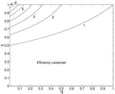
FIG. 2.: Relative efficiency gain $\eta^{e}/\eta$ contours for the three-level ($N=3$) copier detection scheme over the basic detector ($N=0$), as a function of detector efficiency $\eta$ and copier efficiency $\varepsilon$, where both detectors and copiers are noiseless ($\xi=0,\mu=-1$). Valid for any photon input probabilities $p$.

To examine how much improvement can be achieved in more detail, consider when the efficiency of the detectors is $\eta=0.6$. This is a typical efficiency for a pretty good single-photon detector at present. This is shown by the solid lines in Fig. 3. Note how quite large efficiency gains are achievable even when the copier efficiency is slightly over the threshold useful value of $5/7\approx 0.714$ (from Eq. (38)), and how adding more copiers easily introduces more gains at first, but after three levels of copiers, adding more becomes a lot of effort for not much gain.

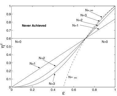
FIG. 3.: Equivalent efficiency $\eta^{e}$, as a function of copier efficiency $\varepsilon$ and number of levels of copiers $N$, when detector efficiency is $\eta=0.6$, and both detectors and copiers are noiseless ($\xi=0$, $\mu=-1$). Results for $N=0$ to $N=3$ are shown as solid lines, and the limit of what can be achieved is shown as a dashed line. Regions beyond the $N=0$ and $N\to\infty$ cases are not achievable with noiseless copiers. Valid for all photon input probabilities $p$.

V The effect of Random Noise on Detection Scheme Usefulness

Following on from the analysis in Sec. IV B, let us now introduce various types of noise into the detection scheme. Unfortunately nice analytical results like (36) - (38) disappear, so what follows is based on the results of numerical calculations. Additionally, the results now also depend on the photon input probabilities $p$.

Firstly consider the effect of dark counts ($\xi\neq 0$), while still keeping the copier noiseless ($\mu=-1$). The regions of efficiency gain and loss with one copier are shown in Fig. 4. In real detectors, dark counts always occur, but are usually kept quite rare, so realistic values of $\xi$ are of the order of $\xi\leqslant 0.01$. Thus (as can be seen from Fig. 4) for likely parameters, dark counts do not reduce the effectiveness of the copier detection scheme by much at all.

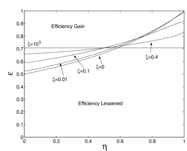
FIG. 4.: Regions of efficiency gain for the single-copier ($N=1$) detection scheme, as a function of $\varepsilon$, the copier, and $\eta$, the detector efficiencies, for varying frequency of dark counts parameterized by $\xi$. In all cases, the copier produces vacuum when it fails ($\mu=-1$) and the input is equiprobable to be a photon or vacuum ($p=1/2$).

Next, consider noise in the copier. In our scheme, noise is linearly introduced into the copying process by varying the parameter $\mu$ away from $|\mu|=1$. The amount of noise increases as $\mu$ approaches zero, until only pure noise occurs upon failure of the copying for $\mu=0$. The dependence on $\mu$ of the values of $\varepsilon$ and $\eta$ needed for efficiency gain is shown in Fig. 5. In the particular case shown, photons and vacuum are equiprobable ($p=1/2$) and there are no dark counts ($\xi=0$).

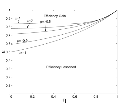
FIG. 5.: Regions of efficiency gain for the single-copier ($N=1$) detection scheme, as a function of $\varepsilon$, the copier, and $\eta$, the detector efficiencies, for varying outputs when the copying fails — i.e. the variation in $\mu$. In all cases, the probability of dark counts in the detectors is taken to be zero ($\xi=0$), and the input is equiprobable to be a photon or vacuum ($p=1/2$). The case $\mu=-1$ corresponds to vacuum output upon failure of copying, $\mu=0$ random output, $\mu=1$ photon output.

Firstly, it is seen that in most cases[12], the optimum output for the copier to produce upon failure is vacuum ($\mu=-1$), and the worst situation is when it produces photons by default ($\mu=1$). Totally random default output ($\mu=0$) requires the copier inefficiency to be reduced by roughly a factor of two relative to what is permissible for vacuum default output. Unfortunately, little is known to date about how much noise will be inevitably introduced in a practical quantum copier, but it seems reasonable that the default output can be made somewhat (perhaps significantly) better than random. If noise could be made 10% probable (perhaps not an unreasonable figure) upon failure to copy, then copiers with efficiency $\varepsilon$ of about $0.65$ would improve detection for typical quantum efficiencies $\eta$ of about $0.3$ or $0.4$. Either way, it is seen that even overwhelming noise upon failure to copy, still allows fairly inefficient (say $\varepsilon\approx 0.8$) copiers to improve the detection efficiency. This is perhaps somewhat unexpected.

Since the effective efficiency $\eta^{e}$ only varies with photon frequency $p$ when noise is present, the next question which arises when considering noisy schemes, is what effect does $p$ have on the performance of the new detection scheme? Fig. 6 shows regions of efficiency increase in terms of $\varepsilon$ and $\eta$ for a single copier scheme, when it is used on sets of input states containing different proportions of photons $p$. The copier in this case produces the maximum amount of noise upon failure (i.e. $\mu=0$). Features seen include

1. Efficiency is easiest to increase when $p$ is close to one, i.e. there are photons coming in most of the time.

2. When photons are rare ($p$ small), the copiers have to be very efficient to be useful, since one wants to register almost all of those that do come along.

3. When photons and vacuum are of a similar frequency, the necessary copier efficiency changes slowly. (see how the $p=0.4,0.5,0.6$ curves are close together).

The behaviour exhibited is fairly typical, although $\mu=0$ appears to be the worst case scenario, as it is the most noisy. In less noisy situations, the required copier efficiency $\varepsilon$ increases more slowly with decreasing $p$.

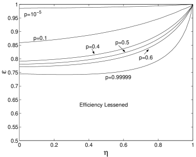
FIG. 6.: Regions of efficiency gain for the single-copier ($N=1$) detection scheme, as a function of $\varepsilon$, the copier, and $\eta$, the detector efficiencies, for varying a priori photon input probabilities $p$. In all cases, the probability of dark counts in the detectors is taken to be zero ($\xi=0$), and the default output upon copy failure is a totally random state ($\mu=0$). Note that the scale in $\varepsilon$ differs from that in Figs. 2, 4, and 5

VI Required Copier Properties

As mentioned briefly at the end of Sec. III (15), the fact that the quantum copier produces entangled states when the input is a superposition is important for the scheme outlined above to work. Let us consider what properties a quantum copier must have to be useful in this scheme.

The scenario where it is easiest to enhance the detection of information is where the detectors are very weak ($\eta$ very small) and there are no dark counts ($\xi=0$). So, if a copier is of no use in this situation, it will not be useful for any detector parameters whatsoever. This will let us specify the broadest range of copier parameters for which they may be useful in improving detection efficiencies.

In any detection situation, we can choose the basis in which to specify the transformation to be the one in which the detectors measure populations only. Since this simplifies the mathematics, let us do so in what follows. We impose one condition on the copier to make the analysis clearer: the states of the copies considered separately (that is, the reduced density matrices of the copies) are identical. This is the usual situation, where both copies are the same. This allows us to write the copying transformation of the two possible input states (including any noise introduced by experimental factors) as

$$\left|{1}\right\rangle\left\langle{1}\right|\to a_{1}\left|{{1}}\right\rangle\!\!\left|{{1}}\right\rangle\left\langle{{1}}\right|\!\!\left\langle{{1}}\right|+a_{2}\left|{{0}}\right\rangle\!\!\left|{{0}}\right\rangle\left\langle{{0}}\right|\!\!\left\langle{{0}}\right|$$ (40)

$$+\frac{1}{2}(1-a_{1}-a_{2})\hat{M}{}+\hat{C}{}_{a},$$ (41)

$$\left|{0}\right\rangle\left\langle{0}\right|\to b_{1}\left|{{1}}\right\rangle\!\!\left|{{1}}\right\rangle\left\langle{{1}}\right|\!\!\left\langle{{1}}\right|+b_{2}\left|{{0}}\right\rangle\!\!\left|{{0}}\right\rangle\left\langle{{0}}\right|\!\!\left\langle{{0}}\right|$$ (42)

$$+\frac{1}{2}(1-b_{1}-b_{2})\hat{M}{}+\hat{C}{}_{b},$$ (43)

where

$$\hat{M}{}=\left|{{0}}\right\rangle\!\!\left|{{1}}\right\rangle\left\langle{{0}}\right|\!\!\left\langle{{1}}\right|+\left|{{1}}\right\rangle\!\!\left|{{0}}\right\rangle\left\langle{{1}}\right|\!\!\left\langle{{0}}\right|,$$ (44)

and where $0\leq a_{1}+a_{2}\leq 1$, $0\leq b-1+b_{2}\leq 1$, and $\hat{C}{}_{a}$, $\hat{C}{}_{b}$ consist only of coherences, so do not contribute to the measurement probabilities, since we have chosen the basis so that what the detectors measure become the populations.

The information about the original states transmitted to the observer with the detectors can be easily calculated using the relations (6), (III), (34), noting that when a copier is present, the POVM which describes the combined measurements at both detectors simply consists of all tensor products of the one-detector POVM

$$\{\hat{A}{}_{nm}=\hat{A}{}_{n}\otimes\hat{A}{}_{m}\ :\ n,m\in\{+,-\}\}.$$ (45)

The information with weak detectors, input photon probability $p$, and no copier is

$$I_{o}(\eta,p)=-\eta p\log_{2}p.$$ (46)

And with copier:

$$I_{m}(\eta, p ,A,B)$$ (47)

$$= \eta pA\log_{2}A+\eta(1-p)B\log_{2}B$$ (49)

$$-\eta[pA+(1-p)B]\log_{2}[pA+(1-p)B],$$

that depends only on two parameters of the copier

$$A=1+a_{1}-a_{2}\quad;\quad B=1+b_{1}-b_{2}.$$ (50)

Fig. 7 shows the values of parameters $A$ and $B$ over which copiers are useful for detection enhancement, for various $p$. Some points to note about this figure:

1. The diagonal $A=B$ corresponds to (via (47)) the worst-case situation where no information about the input states is recoverable from the detectors ($I_{m}=0$).

2. When $A>1$, photon inputs create photon outputs more often than vacuum, while if $B<1$, vacuum inputs create vacuum outputs more often than photons. Thus, the region $A>1$,$B<1$ corresponds to imperfect cloning transformations, while the region $A<1$,$B>1$ corresponds to imperfect ’swapping’ transformations which most often transform photons into vacuum, and vacuum into two photons.

3. Relabeling $\left|{1}\right\rangle\to\left|{0}\right\rangle$, and $\left|{0}\right\rangle\to\left|{1}\right\rangle$ in the copying transformation does not keep the recovered information $I_{m}$ invariant because the detectors do not react the same way to photons and vacuum. This is why Fig. 7 is not symmetric about $A=B$.

4. The noisy copying transformation (III) used in previous sections of this article can be made to correspond to any values of $A$ and $B$ where $A>B$ by appropriate choices of $\mu$ and $\varepsilon$. In fact,

   $$A = 1+\mu+\varepsilon(1-\mu),$$ (52)

   $$B = 1+\mu-\varepsilon(1+\mu),$$ (53)

   and families of such transformations with a set efficiency $\varepsilon$ are parallel to the dividing line $A=B$.

5. Greater ranges of copiers become useful as $p$ (the a priori input photon frequency) becomes larger. For very low photon frequencies, only the close vicinity of $(A,B)=(2,0)$ gives improvements.

6. The Wootters-Zurek copying machine (or entangler) lies at this point $(A,B)=(2,0)$, and is the only copying transformation which gives improvement for arbitrary photon frequency $p$.

7. The well known Universal Quantum Copying Machine (UQCM)[7], which reproduces an arbitrary qubit with the best fidelity lies at $(A,B)=(5/3,1/3)$, outside the region of detection improvement for any $p$, and hence is never useful for the type of detection enhancement scheme discussed here.

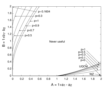
FIG. 7.: Quantum copier properties which allow improvements in information transfer when using detectors of very low efficiency $\eta$ having no dark counts ($\xi=0$). $A$ and $B$ are parameters of the copiers, and the lines show boundaries of the regions in $(A,B)$ space within which copiers give improvements. Various lines correspond to various a priori input photon probabilities $p$ indicated on the plot. Improvements occur in the regions away from the diagonal $A=B$ relative to the boundary lines for a given $p$. For higher efficiencies $\eta$, smaller regions of $A-B$ parameter space are useful. The UQCM is indicated by the cross at $(A,B)=(5/3,1/3)$, and the Wootters-Zurek copier by the circle at $(2,0)$.

Thus one can see that quantum copying transformations used in such a detection improvement scheme as outlined here must be similar in their properties to the Wootters-Zurek copier (the controlled-NOT gate), and the degree of similarity required depends on the input photon frequency.

VII Conclusions

We have provided an example of how spreading information about quantum states onto a larger number of subsystems, actually increases the amount of information about the original state that is available to an observer. The key reason why this occurs is that in realistic situations, observers are always restricted in how close to the ideal their measurements can be. Then, quantum copying the original state may allow the observer to make better use of the detection apparatus at their disposal.

In particular, more efficiency of detection can be gained by employing entangling quantum copiers such as a controlled-NOT gate. In fact if the efficiency of the detectors is far from 100% (such as in single-photon detection) the copier does not have to be very efficient itself, and significant gains in detection can still be made.

From Fig. 2, and others, it can be seen that to be useful, the quantum copiers must be successful with an efficiency $\varepsilon$ over 50% and somewhat greater than the detector efficiency $\eta$. It is not generally clear how feasible this is for various physical systems, or measurement schemes that one might wish to employ. With current technology it is often still easier to make measurements on a system, rather than entangling it with other known systems, however this varies from measurement to measurement and from system to system. The physical processes involved in measurement and quantum copying are often quite different: the former requires creating a correlation between a quantum system and a macroscopic pointer, whereas the latter involves creating quantum entanglement between two similar microscopic states. Efficient detection depends on correlating the system with its environment in a strong, yet controlled way, whereas quantum copying depends on isolating the system from its environment. One thus supposes that the usefulness of a scheme such as the one outlined here will depend on the system and measurements in question, due to the relative ease of implementing detection and controlled quantum evolution in those systems.

The copier parameters required for usefulness of the proposed scheme when random noise is present are found to depend somewhat on the relative frequency of the various states to be distinguished. In any case, the copying transformation must be similar to a controlled-NOT gate, the exact degree of similarity depending on the relative frequency of the input states. The effectiveness of the scheme is, however, quite robust to random noise in the detection and copying. We note that although a detailed analysis was carried out for the case of single-photon detection, the basic scheme immediately generalizes to the case of distinguishing between any two mutually orthogonal states with inefficient detectors, and can be readily generalized to a larger set of input states, and different detectors.

The analysis that is carried out in terms of mutual information between the sequence of input states, and an observer using the detection scheme, is seen to be a simple to use, and powerful method of evaluating detection schemes.

- [1] Email address: deuar@physics.uq.edu.au
- [2] P. Deuar and W. J. Munro, Phys. Rev. A 61, 010306(R) (2000).
- [3] W. K. Wootters and W. H. Zurek, Nature (London) 299, 802 (1982).
- [4] H. Barnum, C. M. Caves, C. A. Fuchs, R. Jozsa, and B. Schumacher, Phys. Rev. Lett. 76, 2818 (1996).
- [5] K. Kraus, States, Effects, and Operations: Fundamental Notions of Quantum Theory (Springer, Berlin, 1983).
- [6] C. M. Caves and P. D. Drummond, Rev. Mod. Phys. 66, 481 (1994).
- [7] V. Bužek and M. Hillery, Phys. Rev. A 54, 1844 (1996).
- [8] C. E. Shannon, Bell Syst. Tech. J. 27, 379 (1948).
- [9] C. E. Shannon, Bell Syst. Tech. J. 27, 623 (1948).
- [10] M. J. W. Hall, Phys. Rev. A 55, 100 (1997).
- [11] P. Deuar and W. J. Munro, Phys. Rev. A (to be published).
- [12] For high detector efficiencies , when dark counts occur, photon default output upon failure to copy () may be more desirable than vacuum.