Experimental realization of optimal detection strategies for overcomplete states

Abstract

We present the results of generalized measurements of optical polarization designed to provide one of three or four distinct outcomes. This has allowed us to discriminate between nonorthogonal polarization states with an error probability that is close to the minimum allowed by quantum theory. Employing these optimal detection strategies on sets of three (trine) or four (tetrad) equiprobable symmetric nonorthogonal polarization states, we obtain a mutual information that exceeds the maximum value attainable using conventional (von Neumann) polarization measurements.

I Introduction

The basic building block in quantum communications and information is the qubit, that is a physical system with two orthogonal quantum states. A simple example is the horizontal and vertical states of polarization associated with a single photon. It is also possible to prepare any superposition of vertical and horizontal polarization and these correspond to other states of linear, circular and elliptical polarization. In quantum communications a transmitting party (Alice) might select from a number of possible nonorthogonal polarization states to send to the receiving party (Bob). This idea is the basis of the emerging technology of quantum key distribution phoenix95a . Signal states with nonorthogonal polarizations may also arise as a result of noisy communications channels acting on orthogonal signal states. For certain types of noisy channels, the throughput of information is actually maximized for nonorthogonal signal states fuchs97a .

The message encoded in the transmitted photons must be retrieved by measurement. This can be achieved either by a conventional (von Neumann) measurement or by means of a generalized measurement holevo73b ; helstrom76a ; peres93a . The von Neumann measurement gives answers corresponding to one of a pair of orthogonal polarization states. The generalized measurements presented in this paper give one of three or four possible outcomes corresponding to the elements of a probability operator measure or POM helstrom76a , also called a positive operator-valued measure peres93a .

If there are only two possible states then it is known that a single von Neumann measurement with two possible outcomes will minimize the probability for error in identifying the state helstrom76a ; sasaki96a . State discrimination with this minimum allowed error probability has been demonstrated for weak pulses of polarized light barnett97a . With only two possible states, it is also possible to discriminate between the two possibilities without error if we allow for the possibility of an inconclusive measurement outcome ivanovic87a ; dieks88a ; peres88a ; jaeger95a ; chefles98a . Near error-free discrimination between two nonorthogonal polarization states was first demonstrated by Huttner et al. huttner96a . More recently, we have shown that it is possible to discriminate between nonorthogonal polarization states clarke00a with the probability for inconclusive outcomes at the quantum limit determined by Ivanovic, Dieks and Peres.

Unambiguous discrimination between two nonorthogonal states of a qubit is an example of a generalized measurement (helstrom76a, ; peres93a, ) in that it requires three possible measurement outcomes but there are only two orthogonal polarizations. Measurements of this kind are required if we wish to perform an optimum measurement on a qubit prepared in more than two different states. In this paper we will describe experiments on polarized light prepared in one of three or four nonorthogonal states. The three states form a so-called trine ensemble holevo73b ; peres92a ; hausladen94a , and take the form of three states of linear polarization separated by an angle of $60^{\circ}$. These states may be represented on the Poincaré sphere born87a as three equidistant points on the equator (see Fig. 1, left). The four states form a tetrad ensemble (davies78a, ) and take the form of two linearly and two elliptically polarized states. These states form the vertices of a tetrahedron on the Poincaré sphere (see Fig. 1, right).

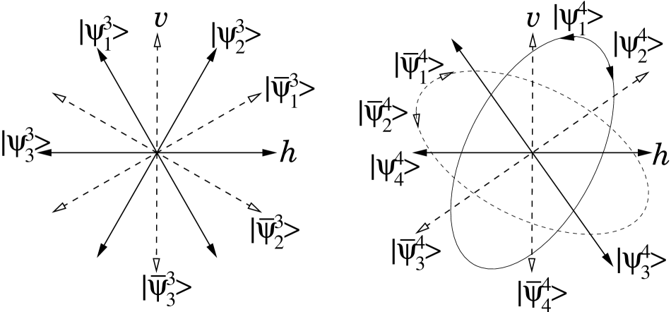
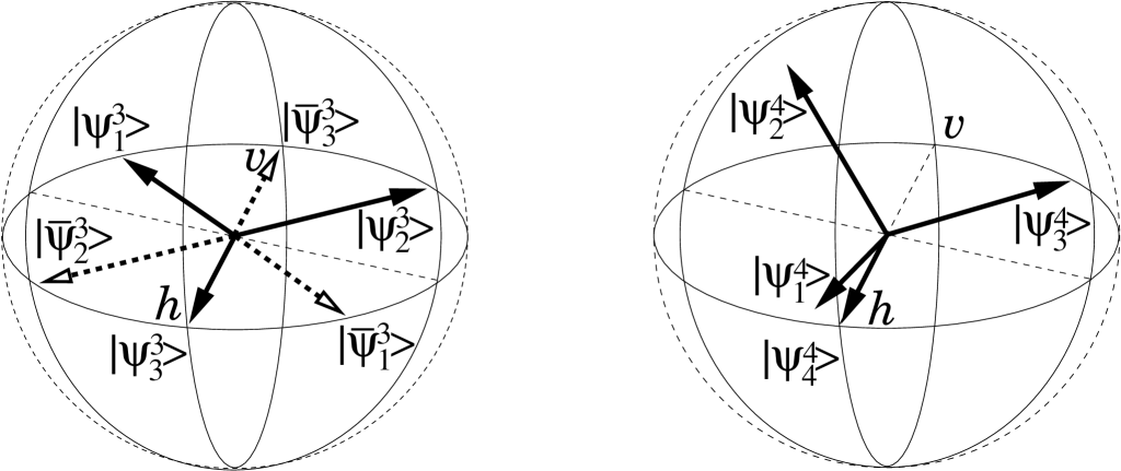
Figure 1: The trine (left) and tetrad (right) states shown as polarization directions (top), and on the Poincaré sphere (shown from two different orientations, middle and lower). Anti-trine (orthogonal) states are also shown (dashed) in the top and middle left diagrams and antitetrad polarization states in the top right diagram.

In this paper we describe our experimental realizations of two types of optimal measurements on these trine and tetrad states. The first gives the minimum probability of error in identifying the state (helstrom76a, ; holevo73a, ; yuen75a, ; phoenix00a, ). The second provides the knowledge that the qubit was definitely not prepared in one out of the three or four possibilities, but does not discriminate further between the remaining possibilities phoenix00a . This measurement is known to give the accessible information (i.e., the mutual information maximized with respect to detection strategy) between transmitter and receiver for equal prior probabilities for the trine states sasaki99a . We calculate the mutual information attainable from our experiments and show that it exceeds that which can be obtained by the best von Neumann measurement.

The rest of the paper is organized as follows. In Section II the relevant theory of probability operator measures (POMs) is outlined. In Section III our implementation of such POMs in optical networks is described theoretically, followed in Section IV by presentation of the experimental setup and results.

II Theory

Consider a communication channel in which photons are prepared, with equal prior probabilities, in one of three or four known states of polarization. Our task is to perform a measurement on the light and so retrieve information about the prepared state. We are interested in two types of measurement. The first is designed to minimize the probability of error in identifying the state correctly, and the second is aimed at maximizing the mutual information associated with the communications channel.

Our signal states are realizations of either the trine holevo73b ; peres92a ; hausladen94a or tetrad davies78a ensembles. The polarization states making up our trine ensemble are

$$|\psi_{1}^{3}\rangle = -\frac{1}{2}\left(|h\rangle+\sqrt{3}|v\rangle\right),$$

$$|\psi_{2}^{3}\rangle = -\frac{1}{2}\left(|h\rangle-\sqrt{3}|v\rangle\right),$$

$$|\psi_{3}^{3}\rangle = |h\rangle,$$ (1)

corresponding to states of linear polarization separated by $60^{\circ}$ (see Fig. 1, left). The kets $|h\rangle$ and $|v\rangle$ are states of horizontal and vertical polarization respectively. The superscript label denotes the fact that there are three members of the trine ensemble. The states making up our tetrad ensemble are

$$|\psi_{1}^{4}\rangle = \frac{1}{\sqrt{3}}\left(-|h\rangle+\sqrt{2}\mathrm{e}^{-2\pi i/3}|v\rangle\right),$$

$$|\psi_{2}^{4}\rangle = \frac{1}{\sqrt{3}}\left(-|h\rangle+\sqrt{2}\mathrm{e}^{+2\pi i/3}|v\rangle\right),$$

$$|\psi_{3}^{4}\rangle = \frac{1}{\sqrt{3}}\left(-|h\rangle+\sqrt{2}|v\rangle\right),$$

$$|\psi_{4}^{4}\rangle = |h\rangle,$$ (2)

where the superscript label again denotes the number of states in the ensemble. The first two states correspond to elliptical polarizations and the second two represent linear polarizations. We also require the states making up the antitrine and antitetrad ensembles. These are the polarization states that are orthogonal to the trine and tetrad states. We denote the members of the antitrine and antitetrad ensembles by an overbar. The members of the antitrine ensemble are

$$|\bar{\psi}_{1}^{3}\rangle = \frac{1}{2}\left(\sqrt{3}|h\rangle-|v\rangle\right),$$

$$|\bar{\psi}_{2}^{3}\rangle = -\frac{1}{2}\left(\sqrt{3}|h\rangle+|v\rangle\right),$$

$$|\bar{\psi}_{3}^{3}\rangle = |v\rangle,$$ (3)

and those of the antitetrad ensemble are

$$|\bar{\psi}_{1}^{4}\rangle = -\frac{1}{\sqrt{3}}\left(\sqrt{2}\mathrm{e}^{2\pi i/3}|h\rangle+|v\rangle\right),$$

$$|\bar{\psi}_{2}^{4}\rangle = -\frac{1}{\sqrt{3}}\left(\sqrt{2}\mathrm{e}^{-2\pi i/3}|h\rangle+|v\rangle\right),$$

$$|\bar{\psi}_{3}^{4}\rangle = -\frac{1}{\sqrt{3}}\left(\sqrt{2}|h\rangle+|v\rangle\right),$$

$$|\bar{\psi}_{4}^{4}\rangle = |v\rangle.$$ (4)

The optimum detection strategies require generalized measurements which may be described in terms of the elements of a POM helstrom76a . Each of the possible results ($y_{j}$) of the measurement corresponds to a Hermitian operator, $\Pi_{j}$, such that the probability of obtaining this result given that the polarization was prepared in the state $|\psi^{N}_{k}\rangle$ is

$$P(y_{j}|\psi^{N}_{k})=\langle\psi^{N}_{k}|\Pi_{j}|\psi^{N}_{k}\rangle,$$ (5)

where $N$ is the number of states making up the ensemble (three for the trine and four for the tetrad).

The requirement that the expectation value of $\Pi_{j}$ is a probability leads to the constraints that all the eigenvalues of $\Pi_{j}$ are positive or zero and that

$$\sum_{j}\Pi_{j}=\openone,$$ (6)

where the sum runs over all possible results of the measurement. This description of a measurement is more general than that associated with a conventional (von Neumann) measurement. For a von Neumann measurement the POM elements are projectors onto the orthonormal eigenstates of the measured observable. In general, however, the POM elements will be neither normalized nor orthogonal.

II.1 Minimum error probability

The problem of finding the measurement which provides the minimum error probability is an old one and it is instructive to present it in a more general form than is strictly necessary for the description of our experiments. Consider a set of possible prepared states with density matrices $\rho_{k}$ and let these occur with prior probabilities $p_{k}$. The lowest error probability will be achieved by a measurement in which we associate a POM element $\Pi_{k}$ with the statement that the prepared state was $\rho_{k}$. The error probability is then

$$P_{e}=1-\sum_{k}p_{k}{\mathrm{T}r}(\rho_{k}\Pi_{k}),$$ (7)

where the sum gives the probability that the state will be correctly identified. The necessary and sufficient conditions on the POM element for this probability to attain its minimum value holevo73a ; yuen75a are

$$\Pi_{j}(p_{j}\rho_{j}-p_{k}\rho_{k})\Pi_{k}=\bm{0}\qquad \forall \,\,(j,k),$$ (8)

$$\left(\sum_{k}p_{k}\rho_{k}\Pi_{k}\right)-p_{j}\rho_{j}\geq\bm{0}\qquad \forall \,\,j.$$ (9)

The general solution for an arbitrary set of states and prior probabilities is unknown but the solution is known for some special cases. We are interested in the pure states making up the trine and tetrad ensembles. These states are overcomplete in that we can resolve the identity as a weighted sum of the corresponding projectors

$$\frac{2}{N}\sum_{k=1}^{N}|\psi_{k}^{N}\rangle\langle\psi_{k}^{N}|=\openone.$$ (10)

If we impose the condition that the states occur with equal prior probabilities then the POM elements that minimize the error probability Eq. (7) are yuen75a ; ban97a

$$\Pi_{k}=\frac{2}{N}|\psi_{k}^{N}\rangle\langle\psi_{k}^{N}|.$$ (11)

This gives for the minimum error probability the value

$$P_{e}(\text{min})=1-\frac{2}{N}.$$ (12)

This is $\frac{2}{3}$ for the trine ensemble and $\frac{1}{2}$ for the tetrad. The remaining problem is to determine how we can design experiments for which the POM elements are those given in Eq. (11). Before addressing this problem we consider another scenario in quantum signal detection.

II.2 Mutual information

The minimum error probability is used as a measure of how precisely one can identify each signal states on average. If instead of identifying each individual state as precisely as possible, one is interested in extracting as much classical information as possible from a sequence of quantum states, a measure commonly used is the Shannon mutual information.

Let us suppose that Alice prepares the ensemble of quantum states $\{|\psi^{N}_{k}\rangle\}$ to encode the classical message $\{x_{k}\}$, where each element appears according to a priori probability $p_{k}$. Let us call this ensemble $X=\{|\psi^{N}_{k}\rangle,p_{k}\}$. The Shannon entropy of $X$ ,

$$H(X)=-\sum_{k}p_{k}\log p_{k},$$ (13)

quantifies how much we know about $X$ just from the a priori probabilities $p_{k}$. Actually, the minimum value of $H(X)$ is zero, corresponding to knowing everything about $X$, and the maximum value of $H(X)$ corresponds to knowing nothing better than a random guess for each element of $X$, so it is more natural to say that $H(X)$ measures what we don’t know about $X$. Bob now applies a measurement with $M$ possible outcomes $\{y_{j}\}$, characterized by the POM elements $\{\Pi_{j}\}$. The outcome, say, $y_{j}$, gives Bob more information about $X$. The new probability distribution conditioned by $y_{j}$ is

$$P(\psi^{N}_{k}|y_{j})=\frac{P(y_{j}|\psi^{N}_{k})p_{k}}{P(y_{j})},$$ (14)

where $P(y_{j})\equiv\sum_{i}P(y_{j}|\psi^{N}_{i})p_{i}$ is the probability of having $y_{j}$, and $P(y_{j}|\psi^{N}_{k})$ is defined by Eq. (5). One can then define the average conditional entropy by

$$H(X|Y)=-\sum_{j}P(y_{j})\sum_{k}P(\psi^{N}_{k}|y_{j})\log P(\psi^{N}_{k}|y_{j}).$$ (15)

This quantifies the remaining uncertainty about $X$ after having the knowledge of the conditioning variable $Y=\{y_{j},P(y_{j})\}$. The information gained as a result of making the measurement $Y$ is naturally defined by

$$I(X:Y) = H(X)-H(X|Y),$$

$$= \sum_{j=1}^{M}\sum_{k=1}^{N}\left[\rule[-13.00005pt]{0.0pt}{25.00003pt}\right.p_{k}P(y_{j}|\psi^{N}_{k})$$

$$\times \left.\log_{2}\left(\frac{P(y_{j}|\psi^{N}_{k})}{\sum_{k^{\prime}=1}^{N}p_{k^{\prime}}P(y_{j}|\psi^{N}_{k^{\prime}})}\right)\right].$$ (17)

This is the Shannon mutual information between $X$ and $Y$. In general, minimizing the average error probability and maximizing the mutual information are different problems, and in fact, one often finds the optimal POMs are different in each case. To extract as much information as possible, Bob has to maximize the mutual information with respect to the POM. The maximum value

$$I_{\rm Acc}=\max_{\{\Pi_{j}\}}I(X:Y),$$ (18)

is called the accessible information of the ensemble $X$. To obtain the accessible information, it is not necessary for the number of measurement outcomes to be the same as the number of signal states. (In the experiments described in this paper, however, these will always be equal.)

The trine and tetrad ensembles comprise nonorthogonal states and hence errors in determining each individual state are inevitable. It is possible, however, to achieve asymptotically error-free transmission of information by employing block coding schemes based on sequences of the states. The accessible information has a practical meaning in this problem. Let $\{\Pi_{j}\}$ be the POM attaining the accessible information for $X$. We consider block sequences of $\{|\psi^{N}_{k}\rangle\}$ of length $n$ and choose $2^{k}$ such sequences (codewords) to code classical messages. Suppose that Bob applies $\{\Pi_{j}\}$ on each states of a received block sequence separately, and guess the codeword sent based on the outcome with any classical procedure. Then if $k/n<I_{\rm Acc}$, Alice and Bob can communicate with an arbitrarily small error by choosing $n$ large enough cover91a .

Thus it is important to find the optimal POM and, in particular, to demonstrate its physical implementation in practice, for developing communication technology though a quantum limited channel. The general problem of finding the accessible information for any given set of signal states remains unsolved. The complete results are known for a few special cases davies78a ; sasaki99a ; osaki00a . For the trine states with equal prior probabilities the accessible information is attained for a measurement with POM elements based on the antitrine states

$$\Pi_{j}=\frac{2}{3}|\bar{\psi}_{j}^{3}\rangle\langle\bar{\psi}_{j}^{3}|.$$ (19)

The optimality of this measurement strategy was conjectured in holevo73a ; peres92a and finally proven by Sasaki et al. sasaki99a . The corresponding accessible information is $\log_{2}\frac{3}{2}=0.585$ bits. This clearly exceeds the value $(-\frac{1}{3}+\frac{1}{2}\log_{2}3)=0.459$ bits which is the maximum mutual information attainable for a von Neumann measurement corresponding to finding one of two orthogonal polarizations.

The accessible information for the tetrad ensemble is not so strongly established as it is for the trine ensemble. Davies davies78a has conjectured that it corresponds to the POM elements

$$\Pi_{j}=\frac{1}{2}|\bar{\psi}_{j}^{4}\rangle\langle\bar{\psi}_{j}^{4}|$$ (20)

associated with the antitetrad states. The mutual information associated with this measurement strategy (conjectured to be the accessible information) is $\log_{2}\frac{4}{3}=0.415$ bits. This again exceeds the value of $\frac{3}{2}(1-\frac{1}{2}\log_{2}3)=0.311$ bits attained for the best possible von Neumann measurement.

It should be noted that the measurement strategy based on the antitrine and antitetrad states only identifies the correct state with probability $1/(N-1)$. However, it obtains more information than the minimum error strategy by identifying for certain one of the states that was not sent.

III Optical implementation

Having described the results that are predicted for various optimal measurements of the trine and tetrad states, we now turn to the implementation of such optimal generalized measurements using specific optical networks to measure photon polarization states. The theoretical operation of the optical networks will be described in the next subsections, followed in Section IV by the description and results of the actual experiments we performed.

The generalized measurements described in the previous section have to be implemented in practice as von Neumann measurements with simple yes/no results, but in an enlarged state space naimark40a ; holevo73a ; helstrom76a ; peres93a . In our experiments, the state space is enlarged by incorporating an interferometer into the measurement apparatus. The enlargement of the state space is realized by the introduction of vacuum modes entering through the unused input port. A single interferometer allows up to four mutually exclusive (orthogonal) possible results from a single photon input state.

In order to describe clearly how our apparatus works, we first set out our sign conventions for the optical components. The main polarizing beam splitters are oriented so that horizontally polarized photons, $|h\rangle$, go straight through, while vertically polarized photons, $|v\rangle$, are deflected through an angle of $\pi/2$. For the non-polarizing beam splitter, the transmission and reflection coefficients are assumed to be equal (both $1/\sqrt{2}$), and since there is only one (non-vacuum) input to it, we take there to be no phase difference between the two outputs. For the quarter and half waveplates, their effect when placed with their fast axis at an arbitrary angle (measured anticlockwise from the horizontal viewed in the direction of travel of the photons) can be described in terms of Jones matrices (see Appendix A). In particular, a half waveplate placed with its axes at an angle of $\pi/4$ to the vertical/horizontal rotates $|v\rangle$ to $|h\rangle$, and $|h\rangle$ to $|v\rangle$, as is well known. A half waveplate with axes at $\pi/8$ to the vertical/horizontal and a quarter waveplate with axes at an angle of $\pi/4$ both produce maximum mixing between the $|v\rangle$ and $|h\rangle$ states, which is what is required to analyze the state obtained when the two arms of the interferometer are recombined. The quarter waveplate is used in the tetrad case, where there is a phase factor of $i$ between the components in each arm. A half waveplate placed at the special angle $\alpha/2=\frac{1}{2}\arcsin(1/\sqrt{3})\simeq 17.63^{\circ}$, is used to rotate the photon until the amplitude of the $|h\rangle$ component is reduced to $\sqrt{2/3}$ of its initial value.

III.1 Trine

An optical network that realizes the minimum error probability for the three trine states is depicted in Fig. 2.

Figure 2: Optical network for the trine generalized measurements. PBS = polarizing beam splitter, WP = waveplate and PD = photodetector (labels correspond with Fig. 4). The dotted lines AA, BB and CC are referred to in the text. The Jones matrix corresponding to each waveplate is shown alongside it ($\Lambda_{2}(\alpha/2)$, etc.) with the angle indicating the orientation of the axes.

This is a variation of recently proposed networks sasaki99a ; phoenix00a . Our trine input states are represented in terms of photon polarization states as in Eq. (1),

$$|\psi^{3}_{1}\rangle = -\frac{1}{2}\left(|h\rangle+\sqrt{3}|v\rangle\right),$$

$$|\psi^{3}_{2}\rangle = -\frac{1}{2}\left(|h\rangle-\sqrt{3}|v\rangle\right),$$

$$|\psi^{3}_{3}\rangle = |h\rangle.$$

After passing through the polarizing beam splitter PBS1, the $|h\rangle$ component of each state goes into the upper arm of the interferometer and the $|v\rangle$ component goes into the lower arm. The half-waveplate WP5 then rotates the $|h\rangle$ component such that at the stage specified by the line AA in Fig. 2, the states have been transformed to

$$|\psi^{3}_{1}\rangle_{\mathrm{A}} = -\frac{1}{2}\frac{1}{\sqrt{3}}\left(\rule[-1.99997pt]{0.0pt}{11.99998pt}\sqrt{2}|h_{\mathrm{U}}\rangle+|v_{\mathrm{U}}\rangle\right)-\frac{\sqrt{3}}{2}|v_{\mathrm{L}}\rangle,$$

$$|\psi^{3}_{2}\rangle_{\mathrm{A}} = -\frac{1}{2}\frac{1}{\sqrt{3}}\left(\rule[-1.99997pt]{0.0pt}{11.99998pt}\sqrt{2}|h_{\mathrm{U}}\rangle+|v_{\mathrm{U}}\rangle\right)+\frac{\sqrt{3}}{2}|v_{\mathrm{L}}\rangle,$$

$$|\psi^{3}_{3}\rangle_{\mathrm{A}} = \frac{1}{\sqrt{3}}\left(\rule[-1.99997pt]{0.0pt}{11.99998pt}\sqrt{2}|h_{\mathrm{U}}\rangle+|v_{\mathrm{U}}\rangle\right),$$ (21)

where the subscripts U and L denote the upper and lower arms of the interferometer respectively. The $|h_{\mathrm{U}}\rangle$ part of these states passes out of the interferometer through PBS2 and into photodetector PD3. If the input state was $|\psi^{3}_{3}\rangle$, there is a probability of $\frac{2}{3}$ that PD3 will detect the photon. If the input state was $|\psi^{3}_{1}\rangle$ or $|\psi^{3}_{2}\rangle$, there is a probability of $\frac{1}{6}$ for each state that PD3 will detect the photon. Turning this round, if PD3 detects the photon, there is a probability of $\frac{2}{3}$ that the input state was $|\psi^{3}_{3}\rangle$ and a probability of $\frac{1}{6}$ each that the input state was $|\psi^{3}_{1}\rangle$ or $|\psi^{3}_{2}\rangle$.

Continuing through the interferometer, the half waveplate WP6 rotates the component in the lower arm from $|v_{\mathrm{L}}\rangle$ to $|h_{\mathrm{L}}\rangle$, so at the stage specified by BB in Fig. 2, the states are

$$|\psi^{3}_{1}\rangle_{\mathrm{B}} = -\frac{1}{\sqrt{6}}|PD3\rangle-\frac{1}{2}\left(\frac{1}{\sqrt{3}}|v_{\mathrm{U}}\rangle+\sqrt{3}|h_{\mathrm{L}}\rangle\right),$$

$$|\psi^{3}_{2}\rangle_{\mathrm{B}} = -\frac{1}{\sqrt{6}}|PD3\rangle-\frac{1}{2}\left(\frac{1}{\sqrt{3}}|v_{\mathrm{U}}\rangle-\sqrt{3}|h_{\mathrm{L}}\rangle\right),$$

$$|\psi^{3}_{3}\rangle_{\mathrm{B}} = \frac{\sqrt{2}}{\sqrt{3}}|PD3\rangle+\frac{1}{\sqrt{3}}|v_{\mathrm{U}}\rangle.$$ (22)

It is necessary to arrange the path lengths in the arms of the interferometer such that there is a relative phase of $\pi/2$ between the U and L components. Then, after the polarizing beam splitter PBS4 recombines the two components, the half waveplate WP9 mixes the two polarizations such that, at the stage indicated by CC on Fig. 2, the states become

$$|\psi^{3}_{1}\rangle_{\mathrm{C}} = -\frac{1}{\sqrt{6}}|PD3\rangle-\frac{1}{\sqrt{3}}\left(\sqrt{2}|h\rangle+\frac{1}{\sqrt{2}}|v\rangle\right),$$

$$|\psi^{3}_{2}\rangle_{\mathrm{C}} = -\frac{1}{\sqrt{6}}|PD3\rangle+\frac{1}{\sqrt{3}}\left(\frac{1}{\sqrt{2}}|h\rangle+\sqrt{2}|v\rangle\right),$$

$$|\psi^{3}_{3}\rangle_{\mathrm{C}} = \frac{\sqrt{2}}{\sqrt{3}}|PD3\rangle+\frac{1}{\sqrt{6}}\left(|h\rangle-|v\rangle\right),$$ (23)

Beam splitter PBS6 separates the $|h\rangle$ and $|v\rangle$ components so they go into detectors PD1 and PD2 respectively. From this we can see that if PD1 detects the photon, there is a probability of $\frac{2}{3}$ that the input state was $|\psi^{3}_{1}\rangle$, and a probability of $\frac{1}{6}$ each that it was $|\psi^{3}_{2}\rangle$ or $|\psi^{3}_{3}\rangle$, similarly for PD2 with states $|\psi^{3}_{1}\rangle$ and $|\psi^{3}_{2}\rangle$ interchanged. In other words, after passing through this optical network, the final states (denoted by subscript F) are given by

$$|\psi^{3}_{1}\rangle_{\mathrm{F}} = -\frac{1}{\sqrt{6}}|PD3\rangle-\frac{\sqrt{2}}{\sqrt{3}}|PD1\rangle-\frac{1}{\sqrt{6}}|PD2\rangle),$$

$$|\psi^{3}_{2}\rangle_{\mathrm{F}} = -\frac{1}{\sqrt{6}}|PD3\rangle+\frac{1}{\sqrt{6}}|PD1\rangle+\frac{\sqrt{2}}{\sqrt{3}}|PD2\rangle,$$

$$|\psi^{3}_{3}\rangle_{\mathrm{F}} = \frac{\sqrt{2}}{\sqrt{3}}|PD3\rangle+\frac{1}{\sqrt{6}}|PD1\rangle-\frac{1}{\sqrt{6}}|PD2\rangle.$$ (24)

This is all normalized so the probabilities are given by the square of the amplitudes of each photodetector state. (The photodetector states $|PD1\rangle$, $|PD2\rangle$ and $|PD3\rangle$ are necessarily mutually orthogonal as only one photodetector out of the three can detect the photon.)

In order to implement the POM corresponding to the maximum mutual information, instead of constructing the optical network that corresponds to POM elements $|\bar{\psi}^{3}_{j}\rangle\langle\bar{\psi}^{3}_{j}|$, and applying it to the trine states, we use the optical network just described (corresponding to the POM elements $|\psi^{3}_{j}\rangle\langle\psi^{3}_{j}|$) and apply it to the antitrine states $|\bar{\psi}^{3}_{j}\rangle$. This is obviously completely equivalent theoretically and more practical experimentally. We find that the state $|\bar{\psi}^{3}_{j}\rangle$ should never trigger photodetector $j$. It will, however, lead to detection in either of the remaining two photodetectors with equal probability ($\frac{1}{2}$) phoenix00a .

III.2 Tetrad

The optical network we used to implements the optimal measurement for the tetrad states is shown in Fig. 3. It is similar to the trine network in Fig. 2, with an extra detector PD4. The key differences are a non-polarizing beam splitter (NPBS) in place of PBS2 and WP5 rotated to an angle of $(\pi/2+\alpha)/2$.

Figure 3: Optical network for the tetrad generalized measurement. NPBS = non-polarizing beam splitter, PBS = polarizing beam splitter, WP = waveplate and PD = photodetector (labels correspond with Fig. 4). The dotted lines AA, BB and CC are referred to in the text. The Jones matrix corresponding to each waveplate is shown alongside it ($\Lambda_{2}(\alpha/2)$, etc.) with the angle indicating the orientation of the axes.

The four tetrad states are represented as polarized photons as in Eq. (2),

$$|\psi^{4}_{1}\rangle = \frac{1}{\sqrt{3}}\left(-|h\rangle+\sqrt{2}\mathrm{e}^{-2\pi i/3}|v\rangle\right),$$

$$|\psi^{4}_{2}\rangle = \frac{1}{\sqrt{3}}\left(-|h\rangle+\sqrt{2}\mathrm{e}^{+2\pi i/3}|v\rangle\right),$$

$$|\psi^{4}_{3}\rangle = \frac{1}{\sqrt{3}}\left(-|h\rangle+\sqrt{2}|v\rangle\right),$$

$$|\psi^{4}_{4}\rangle = |h\rangle.$$

The tetrad network can be understood most straightforwardly by noting the effect of the half waveplate, WP5, on each of the four tetrad states. Denoting the operation of WP5 by the Jones matrix $\Lambda_{2}(\pi/4+\alpha/2)$,

$$\Lambda_{2}(\pi/4+\alpha/2)|\psi^{4}_{1}\rangle = i|\psi^{4}_{2}\rangle,$$

$$\Lambda_{2}(\pi/4+\alpha/2)|\psi^{4}_{2}\rangle = -i|\psi^{4}_{1}\rangle,$$

$$\Lambda_{2}(\pi/4+\alpha/2)|\psi^{4}_{3}\rangle = |\psi^{4}_{4}\rangle,$$

$$\Lambda_{2}(\pi/4+\alpha/2)|\psi^{4}_{4}\rangle = |\psi^{4}_{3}\rangle,$$ (25)

so that, apart from phase factors, state $|\psi^{4}_{1}\rangle$ is converted into $|\psi^{4}_{2}\rangle$ and vice versa, similarly for states $|\psi^{4}_{3}\rangle$ and $|\psi^{4}_{4}\rangle$. Remembering the first beam splitter is $50/50$ non-polarizing, the network is thus essentially symmetrical in its operation. The full details are given in Appendix B. The final result is that state $|\psi^{4}_{1}\rangle$ reaches photodetector PD1 with probability $\frac{1}{2}$ and each of the remaining photodetectors with probability $\frac{1}{6}$. Similarly each of the remaining three states will trigger its associated photodetector with probability $\frac{1}{2}$ and the others with probability $\frac{1}{6}$.

The maximum mutual information measurement is realized in the same way as for the trine ensemble, by using the antitetrad states as input. If the antitetrad states are introduced into this network then we find that the state $|\bar{\psi}^{4}_{j}\rangle$ should never trigger photodetector $j$. It will, however, lead to detection in any of the remaining three photodetectors with equal probability ($\frac{1}{3}$).

IV Experiments

Figure 4: Experimental setup for trine and tetrad state measurements. See text for full description. L = lens, ND = neutral density filter to attenuate the light, NPBS = non-polarizing beamsplitter, PBS = polarizing beam splitter, PD = photodetector, TS = Titanium-Sapphire laser, WP = waveplate, either half or quarter.

Figure 4 shows the experimental arrangements used for the trine and tetrad experiments. The apparatus was easily converted between the two experiments by changing WP7 from a half to a quarter waveplate and exchanging PBS2 with NPBS. We first discuss the general arrangement and techniques that are common to both experiments (see also Ref. clarke00a , where the same experimental setup is described in more detail). The individual details and results of the two experiments are then described separately in Sections IV.1 and IV.2.

The light source was a mode-locked light Ti:Sapphire laser operating at 780 nm with a repetition rate of 80.3 MHz. The pulse duration of 1 ps corresponds to a pulse length of 300 $\mu$m. The repetition rate of the laser ensured that there was only one pulse in the optical system at any one time. The length of each pulse was much shorter than the path length of the interferometer. This meant that each pulse could only interact with one optical component at a time.

The laser light was passed through a 60 $\mu$m pinhole to produce a spherical wavefront. Lens L2 then focused the light onto the photodiodes PD1-5 (Centronix, BPX65) through the interferometer. This arrangement minimized the phase distortions across the wavefront as it passed through the non-ideal interfaces of the beamsplitters, maximizing the visibility of the interference. The focus on the detectors was much smaller than the 1 mm² detector area, yielding almost 100% spatial collection of the light. Losses due to the anti-reflective coatings on the beamsplitters were also small, so almost all the photons entering the interferometer reached the detectors.

The Rochon polarizing beamsplitter PBS1 was used to polarize the light with a linearity of better than 5000:1. The Wollaston polarizing beamsplitter PBS6 was chosen for its similar efficient polarizing properties. The waveplates WP2-4 were then used to prepare the input states, see Appendix A.

In these experiments, we measure the average current from the photodiodes rather than counting discrete photon events. To detect the small quantities of light, phase sensitive detection horowitz89a was employed using a chopper wheel, differential amplifier and a lock-in amplifier. The differential amplifier was used to reduce the noise of the signal by canceling out common ground loop noise using a darkened detector. The detectors PD1-5 had a nominal quantum efficiency of 83% at 780 nm and were terminated by 10 M$\Omega$. At an average laser intensity of 0.1 photons per pulse this corresponds to a detected voltage of 11 $\mu$V. With time constants of 10 to 30 seconds, light levels of 0.01 photons per pulse were detectable with an accuracy of approximately 1% and an uncertainty of approximately $\pm$2.5%.

Neutral density filters and rotation of the waveplate WP1, in conjunction with PBS1, attenuated the light entering the interferometer to an average of 0.1 photons per pulse. A pick-off beam was measured on PD6 using phase sensitive detection with a separate lock-in amplifier. This photodiode was used to normalize output amplitude variations of the laser light when monitoring PD1-5 during all measurements and calibrations. These detectors, supplied in parallel by a single 9 V source, were calibrated relative to each other to better than 1% by changing the distribution of light around the interferometer.

All the waveplates used in the experiments were housed in specially designed mounts. The waveplate was freely rotated to zero its position, measured optically, and locked in position. It could subsequently be moved by predefined fixed angles, including $17.63^{\circ}$ and $27.37^{\circ}$, with an accuracy of $\pm 0.05^{\circ}$ and repeatability of $\pm 0.01^{\circ}$. This enabled quick and accurate changes to the input polarization states in the trine and tetrad experiments. The waveplates were measured to maintain the linearity of the polarization to 1 part in 2000.

The interferometer for the trine experiment was identical to that described in clarke00a . It was constructed from four polarizing beamsplitters mounted on a machined monolithic aluminum block. In a conventional Mach-Zehnder operation, the extinction ratio of the output of the interferometer on detectors PD1 and PD2 was regularly measured to be 200:1. The system was stable enough to be left for over half an hour without significantly impairing this extinction ratio.

For the tetrad experiment the first beamsplitter, NPBS, was non-polarizing with a nominally equal splitting ratio at 780 nm. As the splitting ratio was highly wavelength dependent, the Ti:Sapphire laser was tuned to obtain the most equal splitting ratio, which was estimated to be $49.5:50.5$.

IV.1 Trine Experiment

The interferometer was aligned by using it as a conventional Mach-Zehnder interferometer, with high light powers ($>>1$ photon per pulse). The input polarization was set to be linear at $45^{\circ}$ to the horizontal and WP5 was rotated to produce vertically polarized light. After alignment, the light entering the interferometer was attenuated to 0.1 photons per pulse and WP5 was rotated by $17.63^{\circ}$ so that the polarization of the horizontal component transmitted by PBS2 was rotated anti-clockwise $35.27^{\circ}$ from the horizontal. This reduced the amplitude of the horizontal component to $\sqrt{2/3}$ of its initial value. The 6 input trine and antitrine states were constructed by rotating waveplate WP2 in 15 degree intervals (WP3,4 are not present in this experiment). The results were obtained by taking measurements for one detector (PD1-3) as the 6 input states were changed. Then the next detector was measured for the same 6 states.

After the relative detector calibrations were taken into account, we normalized the results for each input state such that the total average measured probability on photodiodes PD1-3 summed to unity. The $\approx$1% total leakage from PBS3 and PBS4 into detectors PD4 and PD5 is not significant. For the purposes of mutual information it is the ratio of counts in photodiodes PD1-3 that is important, because it is these detectors that distinguish between the input states. The results are shown in Fig. 5.

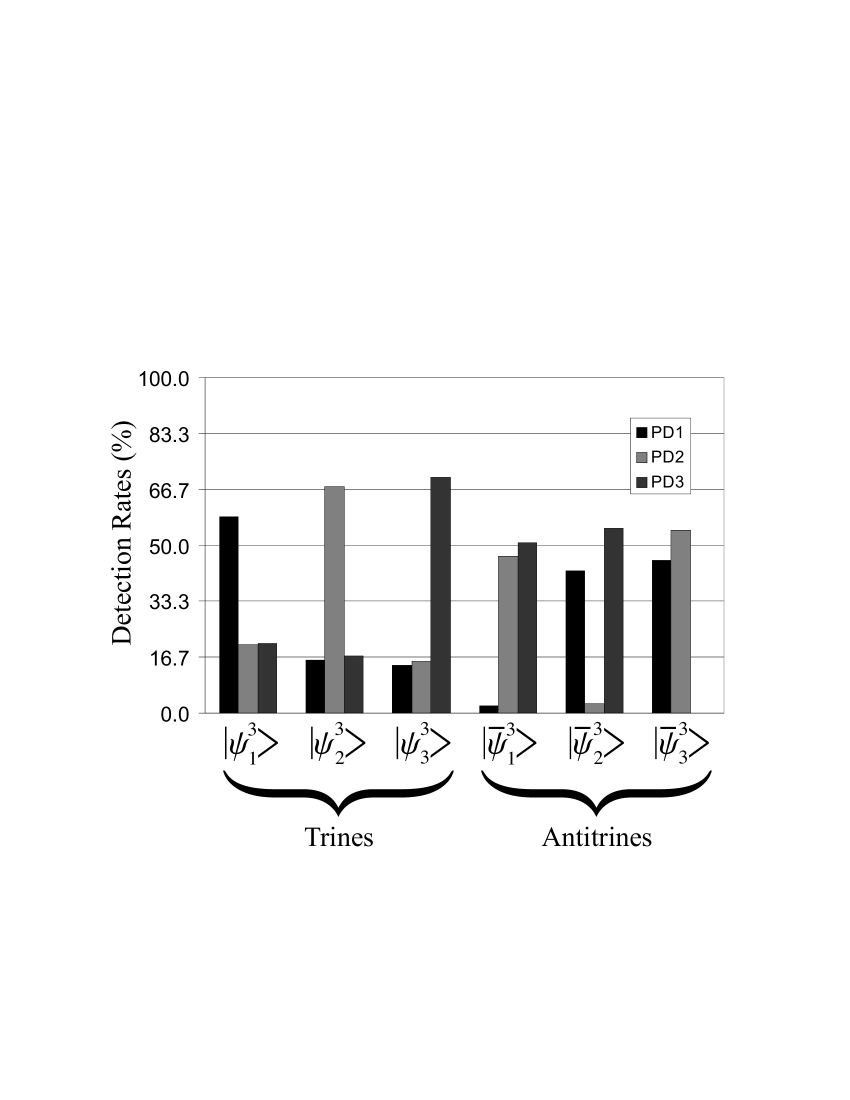
Figure 5: Histogram showing the trine and antitrine results. Normalization ensures the sum of counts in detectors 1, 2 and 3 is $100\%$ for each input state. The theoretical ratios are $\frac{2}{3}:\frac{1}{6}:\frac{1}{6}$ for the trine and $\frac{1}{2}:\frac{1}{2}:0$ for the antitrine states.

The dependence of the measurements on the angle of WP5 was then investigated. The experiment was repeated as the angle of the WP5 was varied either side of the theoretical value of $17.63^{\circ}$. The alignment of the interferometer was checked and adjusted, if necessary, before taking data at each separate angle. Figure 6 shows the root mean squared deviation of the 18 trine and antitrine measurements from the ideal values for each angle.

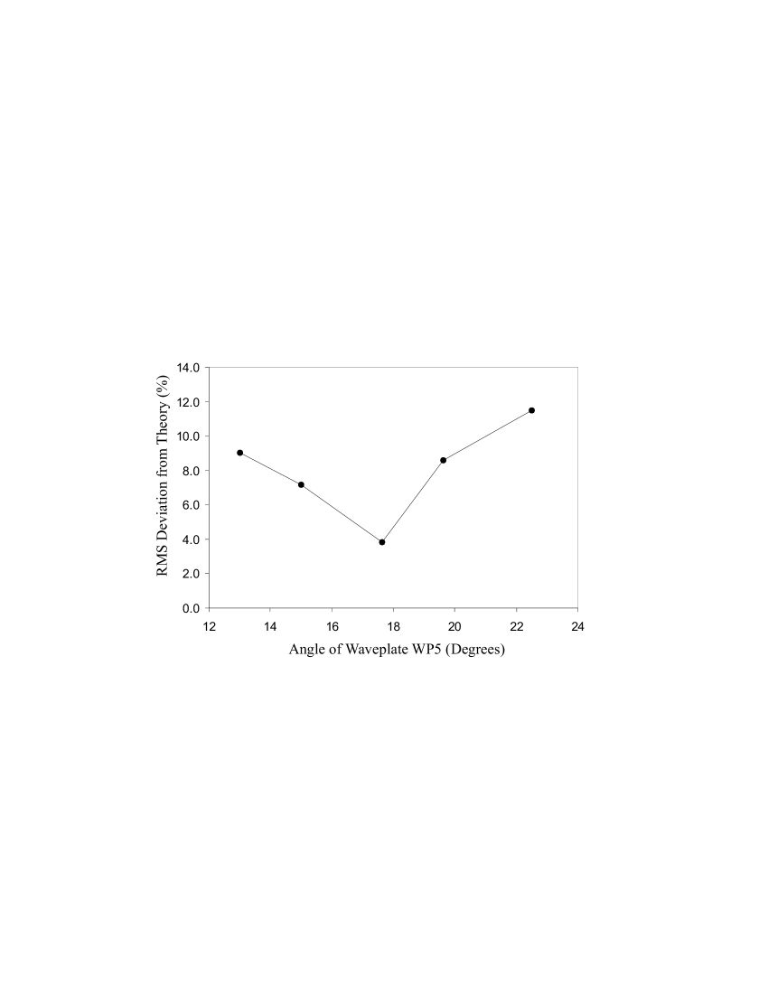
Figure 6: The angle of WP5 is varied around the theoretical value of $\alpha/2=17.63^{\circ}$. The graph shows the RMS deviation of the results from the optimum theoretical results.

Before we discuss the results it is useful to review the sources of error. The largest is the noise of the detector signal and from the phase sensitive detection processing. The observed uncertainty in the measurements of the output ports where a zero count rate is expected in the antitrine experiment is approximately $2.5\%$. This level of error is often similar to the average signal present. We therefore conclude that the zero count measurements are limited by the detector noise if the measured signal is of order 2%. This has important implications for the errors in the derived mutual information, see Section IV.3. The noise is mainly attributable to the weakness of these signals in comparison to the magnitude of ground loop and stray light noise, and also variations in the chopping wheel frequency leading to varying offsets. We estimate that the error due to the amplitude normalization procedure involving PD6 is less than 0.5%, which is much smaller than the Ti:Sapphire amplitude variations of up to 4% over a few minutes.

A second large source of error is the non-ideal nature of the beamsplitters. The calibrated birefringence properties are given in clarke00a . It is sufficient here to state that when purely horizontal light is input into PSB3, a power leakage of approximately 0.9% towards PBS4 was measured. Even this small amount of reflected light can have large effects on the ratio of light reaching detectors PD1 and PD2 due to interference effects.

The drift of the interferometer during measurements was negligible compared to the above errors. This was evaluated by monitoring the level of destructive interference that could be observed on detectors PD1 and PD2 over several hours using high light intensities.

The results in Fig. 5 demonstrate that the trine and antitrine measurements are in close agreement with theoretical predictions. The ratios $\frac{2}{3}:\frac{1}{6}:\frac{1}{6}$ and $\frac{1}{2}:\frac{1}{2}:0$ are clearly visible for the respective measurements. The RMS deviation of the trine and antitrine results is 3.8% from the theoretically expected values. Of specific importance are the antitrine measurements which are theoretically expected to be zero. The experimental measurements are indeed very close to zero, with an average value of 1.6%. Fig. 6 also shows that the minimum RMS error from the optimum theoretical values was obtained when the waveplate WP5 was at the angle corresponding to the theoretical value, within the limits imposed by the small number of data points.

Close inspection of Fig. 5 demonstrates the effect of the leakage of PBS3. For antitrine input state $|\psi^{3}_{3}\rangle$ the light on PD1 and PD2 is split into the ratio 46:54. In an ideal experiment there would be no light traveling towards PBS4 from PBS2 and the split would be 50:50. Indeed, this ratio is observed to better than $\pm 0.2\%$ if an opaque card is placed between PBS2 and PBS4. The leakage from PBS2, when interfering with the light from PBS3, is enough to skew the results by 8%. This demonstrates the sensitivity of the apparatus to practical sources of error.

IV.2 Tetrad Experiment

The first beamsplitter PBS1 in the interferometer was changed to a non-polarizing beamsplitter. Alignment of the interferometer was achieved by simulating a conventional Mach-Zehnder operation with vertically polarized input light. Waveplate WP5 was aligned with the slow axis in the vertical direction and WP7, a quarter waveplate, rotated so that there was complete mixing of the output states of the interferometer.

After the alignment, waveplate WP5 was rotated clockwise by $54.74^{\circ}/2=27.37^{\circ}$. This corresponds to setting the fast axis at $125.26^{\circ}/2=54.747^{\circ}$ anti-clockwise from the horizontal. The angle between two tetrad states is $125.26^{\circ}$ on the Poincaré sphere, or $54.74^{\circ}$ in polarization.

The four tetrad and four antitetrad polarization states required to perform this experiment were constructed using waveplates WP2-4 as described in Appendix A. We were able to change between the 8 input states in a matter of seconds using the discrete predefined angles in our waveplate holders.

The experiment was performed by measuring the signal on detectors PD1-4 as the input states were changed between the 8 states. The results of the tetrad and antitetrad measurements are shown in Figs. 7 and 8 after calibration and normalization.

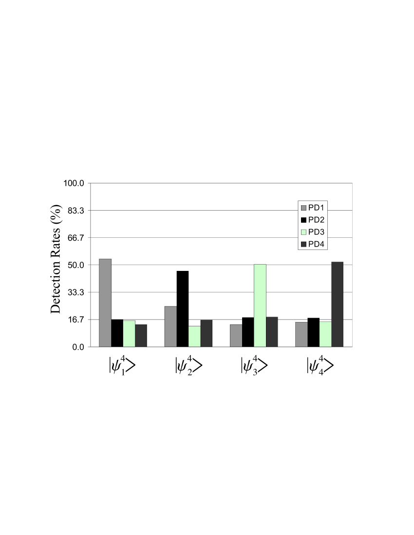
Figure 7: Histogram showing the tetrad results, normalized so that the sum of the counts in detectors 1 to 4 is $100\%$ for each input state. The theoretical ratios are $\frac{1}{2}:\frac{1}{6}:\frac{1}{6}:\frac{1}{6}$.

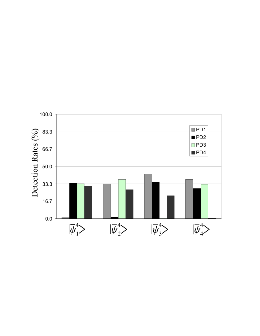
Figure 8: Histogram showing the antitetrad results, normalized so that the sum of the counts in detectors 1 to 4 is $100\%$ for each input state. The theoretical ratios are $\frac{1}{3}:\frac{1}{3}:\frac{1}{3}:0$.

As with the trine measurements, it is clear that the experimental results are in good agreement with the theoretical predictions. The $\frac{1}{2}:\frac{1}{6}:\frac{1}{6}:\frac{1}{6}$ and $\frac{1}{3}:\frac{1}{3}:\frac{1}{3}:0$ ratios for the tetrad and antitetrad states respectively are clearly evident. The overall RMS deviation from the theoretical values is 2.9%. Attention is drawn to the antitetrad states where the count rate is theoretically zero. The average count rate in these four measurements is 0.9%. This low count rate is very significant for the mutual information that can be obtained, see next subsection.

IV.3 Experimental Mutual Information

The mutual information for both experiments was calculated in bits (log₂) using Eq. (17). The conditional probabilities were obtained from the experiment. The values for $p_{k}$ were set to $\frac{1}{3}$ and $\frac{1}{4}$ for the trine and tetrad cases respectively, corresponding to equal prior probabilities for the input states. The results, summarized in Table 1, are in excellent agreement with the theoretical predictions using the model for detector noise described in Appendix C. The mutual information of both sets of antistates is significantly greater than the best possible von Neumann measurement.

States	Experiment	Ideal Theory	Noisy Theory	von Neumann
trine	0.312 ${}^{+0.017}_{-0.08}$	0.333	0.302	0.459
antitrine	0.491 ${}^{+0.011}_{-0.027}$	0.585	0.486	0.459
tetrad	0.209 ${}^{+0.013}_{-0.010}$	0.208	0.194	0.311
antitetrad	0.363 ${}^{+0.09}_{-0.024}$	0.415	0.355	0.311

Table 1: Mutual information expressed in bits for the trine and tetrad states and their antistates. The values indicate the mutual information obtained in the experiment, in an ideal experiment, in an ideal experiment with detector noise analyzed using the error model described in Appendix B, and the maximum allowed mutual information in a von Neumann measurement.

Experimental errors were estimated in a Monte Carlo simulation, assuming a flat $\pm$2.5% error distribution in the measurements. The theoretical sensitivity of the mutual information to measurement error was estimated using a simple error model, see Appendix C. The parameter, $\Gamma$, was used to quantify the level of noise. The average signal of the near-zero measurements in the trine and tetrad experiments, 1.6% and 0.9% respectively, was used to obtain the parameter $\Gamma=0.952$ and $0.964$ respectively.

In the antitrine and antitetrad cases it was found that the sensitivity of the mutual information obtained is almost entirely determined by the noise-induced counts at the detector that would, in an ideal experiment, register no counts. This is a consequence of the logarithmic nature of the mutual information. In an ideal experiment, a count in detector PD$j$ means that state $|\bar{\psi}^{N}_{j}\rangle$ was definitely not the input state. The knowledge of the input state has therefore been increased by a large amount. Any deviation from theoretically zero count rates in the experiment will lead to a rapid increase in the errors associated with this deduction. Hence, the mutual information will decrease rapidly. Nevertheless, in our experiments, the mutual information obtained for both the antitrine and antitetrad states is still significantly higher than the best possible von Neumann measurement. To our knowledge this is first time this has been achieved experimentally. Measurement errors due to noise are the limiting factor determining the mutual information that can be achieved experimentally. The largest source of noise is due to ground loop noise in the detectors. The use of single photon detectors gated with the pulses of light should reduce this noise considerably and yield further increases in the mutual information obtained.

V Conclusions

In quantum communications the possible signal states can be nonorthogonal. This leads to problems in recovering the signal by detection. In general, we must accept the presence of errors. We have realized detection strategies that either minimise the error probability or maximise the mutual information for the trine and tetrad states. The mutual information is an important parameter in communications, quantifying the maximum amount of information that can be extracted from a signal. In the context of measuring the polarization of light, probability operator measures provide a means of attaining higher mutual information values than von Neuman measurements. We have presented two separate experiments using heavily attenuated pulses of light to verify the optimal POM on trine and tetrad polarization states of light. We have demonstrated for the first time that the mutual information obtainable using POMs can be significantly higher than the maximum possible mutual information in a von Neuman measurement. This illustrates the principle that generalised measurements can be of greater utility than their more familiar von Neuman counterparts.

Using a flexible free space interferometer we were able to vary all aspects of the measurement process deterministically. The mutual information is extremely sensitive to the noise of the detectors in which very low counts rates are expected. We have demonstrated that practical communications using POMs are feasible.

Appendix A Making an arbitrary polarization state

The convention used for the orientation of the waveplates is as follows. Viewed in the direction of propagation, the fast axis of the waveplate makes an angle $\phi/2$ with the horizontal in an anti-clockwise direction, and the slow axis similarly makes an angle $\phi/2$ with the vertical. Expressed in Jones matrix notation hecht87a , the action of a half waveplate is thus

$$\Lambda_{2}(\phi/2)\left(\begin{array}[]{c}h\\ v\\ \end{array}\right)=\left(\begin{array}[]{cc}\cos\phi&\sin\phi\\ \sin\phi&-\cos\phi\\ \end{array}\right)\left(\begin{array}[]{c}h\\ v\\ \end{array}\right),$$ (26)

where $h$ and $v$ are the amplitudes of horizontal and vertical polarization in the state respectively. Similarly, the action of a quarter waveplate with its fast axis at an angle $\theta/2$ to the horizontal is

$$\Lambda_{4}(\theta/2)\left(\begin{array}[]{c}h\\ v\\ \end{array}\right)$$ (29)

$$=\left(\begin{array}[]{cc}\sin^{2}(\theta/2)+i\cos^{2}(\theta/2)&\frac{i-1}{2}\sin\theta\\ \frac{i-1}{2}\sin\theta&\cos^{2}(\theta/2)+i\sin^{2}(\theta/2)\\ \end{array}\right)\left(\begin{array}[]{c}h\\ v\\ \end{array}\right)$$ (34)

$$=\frac{1}{\sqrt{2}}\left(\begin{array}[]{cc}\cos\theta-i&\sin\theta\\ \sin\theta&-\cos\theta-i\\ \end{array}\right)\left(\begin{array}[]{c}h\\ v\\ \end{array}\right),$$ (39)

where the overall phase of $e^{i3\pi/4}$ has been dropped.

As can easily be verified using the above expressions, an arbitrary polarization state can be made from horizontally polarized input light using a sequence of three waveplates, quarter-half-quarter, at the appropriate angles, see Fig. 9.

Figure 9: Optical arrangement for making an arbitrary state. Waveplates WP2 and WP4 are quarter waveplates and WP3 is a half waveplate.

If the input state is $|h\rangle$ (horizontal polarization), and the orthogonal polarization is $|v\rangle$, the output state, $|\psi\rangle$, is given by

$$|\psi\rangle=\cos\beta\,|h\rangle+\mathrm{e}^{i\gamma}\sin\beta\,|v\rangle,$$ (40)

where $\sin\phi=-\sin\beta\,\sin\gamma$ and $\tan\theta=\tan\beta\,\cos\gamma$, with $\theta$, $\phi$ specifying the orientation of the three waveplates as given in Fig.9.

Appendix B Details of tetrad optical implementation

Starting from the input states given by Eq. (2), at the stage indicated by the line AA on Fig. 3, we have

$$|\psi^{4}_{1}\rangle_{\mathrm{A}} = \frac{1}{\sqrt{2}}\left(|\psi^{4}_{1}\rangle_{\mathrm{L}}+i|\psi^{4}_{2}\rangle_{\mathrm{U}}\right),$$

$$|\psi^{4}_{2}\rangle_{\mathrm{A}} = \frac{1}{\sqrt{2}}\left(|\psi^{4}_{2}\rangle_{\mathrm{L}}-i|\psi^{4}_{1}\rangle_{\mathrm{U}}\right),$$

$$|\psi^{4}_{3}\rangle_{\mathrm{A}} = \frac{1}{\sqrt{2}}\left(|\psi^{4}_{3}\rangle_{\mathrm{L}}+|\psi^{4}_{4}\rangle_{\mathrm{U}}\right),$$

$$|\psi^{4}_{4}\rangle_{\mathrm{A}} = \frac{1}{\sqrt{2}}\left(|\psi^{4}_{4}\rangle_{\mathrm{L}}+|\psi^{4}_{3}\rangle_{\mathrm{U}}\right).$$ (41)

In terms of $|h\rangle$ and $|v\rangle$,

$$|\psi^{4}_{1}\rangle_{\mathrm{A}} = \frac{1}{\sqrt{6}}\left(-|h_{\mathrm{L}}\rangle+\sqrt{2}\mathrm{e}^{-2\pi i/3}|v_{\mathrm{L}}\rangle-i|h_{\mathrm{U}}\rangle\right.$$

$$+i\sqrt{2}\mathrm{e}^{2\pi i/3}|v_{\mathrm{U}}\rangle\left.\mbox{\rule[-1.99997pt]{0.0pt}{11.99998pt}}\right),$$

$$|\psi^{4}_{2}\rangle_{\mathrm{A}} = \frac{1}{\sqrt{6}}\left(-|h_{\mathrm{L}}\rangle+\sqrt{2}\mathrm{e}^{2\pi i/3}|v_{\mathrm{L}}\rangle+i|h_{\mathrm{U}}\rangle\right.$$

$$-i\sqrt{2}\mathrm{e}^{-2\pi i/3}|v_{\mathrm{U}}\rangle\left.\mbox{\rule[-1.99997pt]{0.0pt}{11.99998pt}}\right),$$

$$|\psi^{4}_{3}\rangle_{\mathrm{A}} = \frac{1}{\sqrt{6}}\left(-|h_{\mathrm{L}}\rangle+\sqrt{2}|v_{\mathrm{L}}\rangle+\sqrt{3}|h_{\mathrm{U}}\rangle\right),$$

$$|\psi^{4}_{4}\rangle_{\mathrm{A}} = \frac{1}{\sqrt{6}}\left(\sqrt{3}|h_{\mathrm{L}}\rangle-|h_{\mathrm{U}}\rangle+\sqrt{2}|v_{\mathrm{U}}\rangle\right).$$ (42)

Then the $|h_{\mathrm{L}}\rangle$ components can reach photo-detector PD4 and the $|h_{\mathrm{U}}\rangle$ components can reach photo-detector PD3, while the $|v_{\mathrm{L}}\rangle$ and $|v_{\mathrm{U}}\rangle$ components continue round the lower and upper arms of the interferometer respectively. Applying WP6 to $|v_{\mathrm{L}}\rangle$, converting it to $|h_{\mathrm{L}}\rangle$, the states at the stage indicated by the line BB in Fig. 3 are

$$|\psi^{4}_{1}\rangle_{\mathrm{B}} = \frac{1}{\sqrt{6}}\left(\sqrt{2}\mathrm{e}^{-2\pi i/3}|h_{\mathrm{L}}\rangle+i\sqrt{2}\mathrm{e}^{2\pi i/3}|v_{\mathrm{U}}\rangle\right.$$

$$-i|PD3\rangle-|PD4\rangle\left.\mbox{\rule[-1.99997pt]{0.0pt}{11.99998pt}}\right),$$

$$|\psi^{4}_{2}\rangle_{\mathrm{B}} = \frac{1}{\sqrt{6}}\left(\sqrt{2}\mathrm{e}^{2\pi i/3}|h_{\mathrm{L}}\rangle-i\sqrt{2}\mathrm{e}^{-2\pi i/3}|v_{\mathrm{U}}\rangle\right.$$

$$+i|PD3\rangle-|PD4\rangle\left.\mbox{\rule[-1.99997pt]{0.0pt}{11.99998pt}}\right),$$

$$|\psi^{4}_{3}\rangle_{\mathrm{B}} = \frac{1}{\sqrt{6}}\left(\sqrt{2}|h_{\mathrm{L}}\rangle+\sqrt{3}|PD3\rangle-|PD4\rangle\right),$$

$$|\psi^{4}_{4}\rangle_{\mathrm{B}} = \frac{1}{\sqrt{6}}\left(\sqrt{2}|v_{\mathrm{U}}\rangle-|PD3\rangle+\sqrt{3}|PD4\rangle\right).$$ (43)

Finally, the maximal mixing effect of WP9 brings the states into

$$|\psi^{4}_{1}\rangle_{\mathrm{C}} = \frac{1}{\sqrt{6}}\left(-i\sqrt{3}|h\rangle-i|v\rangle-i|PD3\rangle-|PD4\rangle\right),$$

$$|\psi^{4}_{2}\rangle_{\mathrm{C}} = \frac{1}{\sqrt{6}}\left(-|h\rangle-\sqrt{3}|v\rangle+i|PD3\rangle-|PD4\rangle\right),$$

$$|\psi^{4}_{3}\rangle_{\mathrm{C}} = \frac{1}{\sqrt{6}}\left(|h\rangle+i|v\rangle+\sqrt{3}|PD3\rangle-|PD4\rangle\right),$$

$$|\psi^{4}_{4}\rangle_{\mathrm{C}} = \frac{1}{\sqrt{6}}\left(i|h\rangle+|v\rangle-|PD3\rangle+\sqrt{3}|PD4\rangle\right),$$ (44)

from which the final outcome is easily seen to be

$$|\psi^{4}_{1}\rangle_{\mathrm{F}} = -\frac{i}{\sqrt{2}}|PD1\rangle-\frac{i}{\sqrt{6}}|PD2\rangle$$

$$+\frac{i}{\sqrt{6}}|PD3\rangle-\frac{1}{\sqrt{6}}|PD4\rangle,$$

$$|\psi^{4}_{2}\rangle_{\mathrm{F}} = -\frac{1}{\sqrt{6}}|PD1\rangle-\frac{1}{\sqrt{2}}|PD2\rangle$$

$$-\frac{i}{\sqrt{6}}|PD3\rangle-\frac{1}{\sqrt{6}}|PD4\rangle,$$

$$|\psi^{4}_{3}\rangle_{\mathrm{F}} = \frac{1}{\sqrt{6}}|PD1\rangle+\frac{i}{\sqrt{6}}|PD2\rangle$$

$$+\frac{1}{\sqrt{2}}|PD3\rangle-\frac{1}{\sqrt{6}}|PD4\rangle,$$

$$|\psi^{4}_{4}\rangle_{\mathrm{F}} = \frac{i}{\sqrt{6}}|PD1\rangle+\frac{1}{\sqrt{6}}|PD2\rangle$$ (45)

$$-\frac{1}{\sqrt{6}}|PD3\rangle+\frac{1}{\sqrt{2}}|PD4\rangle,$$

where the amplitudes give the probabilities of each photodetector finding the photon.

Appendix C Mutual Information Error Model

The mutual information obtained is very sensitive to noise. In this appendix we present a simple model for detector noise and use it to analyze our measurements of mutual information. Rather than attempt to account for all sources of noise, our model simply assumes that the noise randomly distributes a proportion of the detection events among all the detectors.

The probability for detecting a photon in detector $j$ (outcome $y_{j}$) is associated with the POM element $\Pi_{j}$. Noise can cause a photocurrent to occur in a detector in the absence of any photons. Such noise-inducing events are randomly distributed and so we can modify our POM elements to account for these noisy events by replacing POM elements $\{\Pi_{j}\}$ for an ideal measurement with

$$\Pi_{j}^{\mathrm{noise}}=\Gamma\Pi_{j}+\frac{1-\Gamma}{N}.$$ (46)

Here $N$ is the number of measurement outcomes and $\Gamma$ is a positive number ($\Gamma\leq 1$) that characterizes the noise. For $\Gamma=1$ there is no noise, but for $\Gamma=0$, noise accounts for all detection events. The conditional probabilities in the presence of noise become

$$P(y_{j}|\psi^{N}_{k})=\langle\psi^{N}_{k}|\Pi_{j}^{\mathrm{noise}}|\psi^{N}_{k}\rangle.$$ (47)

Given a channel in which the input states $|\psi^{N}_{k}\rangle$ occur with equal probability we find that the mutual information becomes

$$I(\{|\psi^{N}_{k}\rangle\}: \{y_{j}\})=\left(\frac{1+\Gamma}{N}\right)\log(1+\Gamma)$$

$$+ \left(1-\frac{1+\Gamma}{N}\right)\log\left(1-\frac{\Gamma}{N-1}\right).$$ (48)

If, instead, the antistates $|\bar{\psi}^{N}_{k}\rangle$ are used as input, the mutual information is

$$I(\{|\bar{\psi}^{N}_{k}\rangle\}: \{y_{j}\})=\left(\frac{1-\Gamma}{N}\right)\log(1-\Gamma)$$

$$+ \left(1-\frac{1-\Gamma}{N}\right)\log\left(1+\frac{\Gamma}{N-1}\right).$$ (49)

It is interesting to note that C and 49 differ in form only through the sign of $\Gamma$.

We can estimate the value of $\Gamma$ by considering the probability for the measurement of the antistate $|\bar{\psi}^{N}_{k}\rangle$ to give the result $y_{k}$, corresponding to “not-$|\bar{\psi}^{N}_{k}\rangle$”. This is forbidden for an ideal, noiseless experiment but will occur with probability $(1-\Gamma)/N$ in the presence of noise. Comparing this with the experimentally observed values provides us with a value for $\Gamma$.

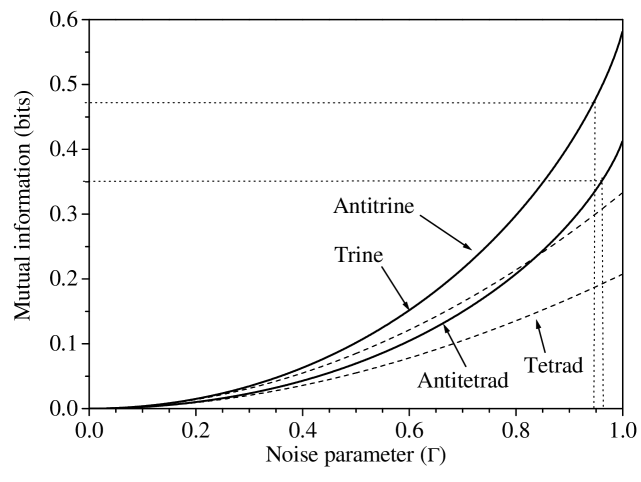
Figure 10: The theoretical variation of the mutual information with the detector noise, given by parameter $\Gamma$, for the trine, antitrine, tetrad and antitetrad states. Included are read-off lines to show the theoretical values of the mutual information for the antitrine and antitetrad measurements, given the experimental values of $\Gamma=0.952$ and $0.964$ respectively.

Figure 10 shows the variation of the mutual information obtained as $\Gamma$ is varied. The sensitivity to noise in the antitrine and antitetrad states increases markedly as $\Gamma$ tends to 1. This demonstrates the sensitivity of the mutual information to noise in the detector which, in an ideal experiment, would register no counts. The mutual information of trine and tetrad measurements does not increase as rapidly because there are no detectors in which zero counts are expected.

References

- (1) S. J. D. Phoenix and P. D. Townsend, Contemp. Phys. 36, 165 (1995), and references therein.
- (2) C. F. Fuchs, Phys. Rev. Lett. 79(6), 1162 (1997).
- (3) C. W. Helstrom, Quantum Detection and Estimation Theory (Academic Press, New York, New York, 1976).
- (4) A. Peres, Quantum Theory: Concepts and Methods (Kluwer Academic Publishers, Dordrecht, Dordrecht, 1993), also called a positive operator-valued measure.
- (5) A. S. Holevo, Problemy Peredachi Informatsii 9, 31 (1973), Problems of Information Transmision (USSR), 9, 110.
- (6) M. Sasaki and O. Hirota, Phys. Rev. A 54(4), 2728 (1996).
- (7) S. M. Barnett and E. Riis, J. Mod. Opt. 44, 1061 (1997).
- (8) I. D. Ivanovic, Phys. Lett. A 123, 257 (1987).
- (9) D. Dieks, Phys. Lett. A 126, 303 (1988).
- (10) A. Peres, Phys. Lett. A 128, 19 (1988).
- (11) G. Jaeger and A. Shimony, Phys. Lett. A 197, 83 (1995).
- (12) A. Chefles and S. M. Barnett, J. Mod. Opt. 45, 1295 (1998).
- (13) B. Huttner, A. Muller, J. D. Gautier, H. Zbinden, and N. Gisin, Phys. Rev. A 54, 3783 (1996).
- (14) R. B. M. Clarke, A. Chefles, S. M. Barnett, and E. Riis, Phys. Rev. A (2001), accepted February 2001.
- (15) A. Peres and W. Wootters, Phys. Rev. Lett. 66, 1119 (1992).
- (16) P. Hausladen and W. K. Wootters, J. Mod. Optics 41(12), 2385 (1994).
- (17) M. Born and E. Wolf, Principles of Optics (Pergamon Press, Oxford, 1987), p.31.
- (18) E. B. Davies, IEEE Trans. Inform. Theory 24, 596 (1978).
- (19) A. S. Holevo, J. Multivariate Analysis 3, 337 (1973).
- (20) H. P. Yuen, R. S. Kennedy, and M. Lax, IEEE Trans. Information Theory 21(2), 125 (1975).
- (21) S. J. D. Phoenix, S. M. Barnett, and A. Chefles, J. Mod. Opt. 47, 507 (2000).
- (22) M. Sasaki, S. M. Barnett, R. Jozsa, M. Osaki, and O. Hirota, Phys. Rev. A 59(5), 3325 (1999).
- (23) M. Ban, K. Kurokawa, R. Momose, and O. Hirota, Int. J. Theor. Phys. 36(6), 1269 (1997).
- (24) T. Cover and J. Thomas, Elements of Information Theory (John Wiley and Sons, New York, 1991).
- (25) M. Osaki, M. Ban, and O. Hirota, in Proceedings of the 4th conference on Quantum Communication, Measurement, and Computating, Evanston, Illinois, USA (1998) (Plenum Press, New York, 2000).
- (26) M. A. Naimark, Izv. Akad. Nauk. SSSR Ser. Mat. 4, 277 (1940).
- (27) P. Horowitz and W. Hill, The Art of Electronics (Cambridge University Press, Cambridge UK, 1989).
- (28) E. Hecht, Optics (Addison-Wesley, Reading, Mass, 1987), 2nd ed., (see, for example p.321 ff).