A sequence of unsharp measurements enabling a real time visualization of a quantum oscillation

Abstract

The normalized state $|\psi(t)\rangle=c_{1}(t)|1\rangle+c_{2}(t)|2\rangle$ of a single two-level system performs oscillations under the influence of a resonant driving field. It is assumed that only one realization of this process is available. We show that it is possible to approximately visualize in real time the evolution of the system as far as it is given by $|c_{2}(t)|^{2}$. For this purpose we use a sequence of particular unsharp measurements separated in time. They are specified within the theory of generalized measurements in which observables are represented by positive operator valued measures (POVM). A realization of the unsharp measurements may be obtained by coupling the two-level system to a meter and performing the usual projection measurements on the meter only.

1 Introduction

Recently, considerable progress has been made in the experimental and theoretical study of single quantum systems in atomic traps and optical cavities as well as in the context of solid-state physics (coupled quantum dots). In many cases the physical situation may be described by means of a two level system with states $|1\rangle$ and $|2\rangle$ under the influence of a periodic driving potential $V(t)$. The resulting motion of the normalized state

$$|\psi\rangle=c_{1}|1\rangle+c_{2}|2\rangle$$ (1)

involves oscillations of the probabilities $|c_{1}(t)|^{2}$ and $|c_{2}(t)|^{2}$ called Rabi oscillations. The usual way to measure the dynamics of $|c_{2}(t)|^{2}$ employs many projection measurements of an observable with eigenstates $|1\rangle$ and $|2\rangle$. For this purpose an ensemble is prepared in the initial state and a projection measurement is carried out at time $t_{0}$ on each member of the ensemble leading to the determination of $|c_{2}(t_{0})|^{2}$. Repeating the procedure for different times $t$ one obtains the Rabi oscillations of $|c_{2}(t)|^{2}$.

This procedure fails if there is only one single quantum system available and the objective is to visualize its motion in real time. Imagine, e.g., there is a single two-level system performing only once a hundred Rabi oscillations. Is there a method to visualize them? There are two complementary conditions such a method must meet. The measurement must not disturb the system too much, so that its evolution remains close to the undisturbed case. On the other hand, the coupling of the measurement apparatus to the two level system should nevertheless be so strong that the readout shows accurately enough the modified dynamics of the system (including the disturbance by the measurement).

This can clearly not be achieved by standard measurements which project onto an eigenstate of the measured observable. They disturb the system too strongly. For instance, the well known Quantum Zeno effect shows that it is possible to detect perfectly the modified dynamics of a system at the price of loosing all information about the undisturbed motion. The measurement disturbs the dynamics so much as to make the system stay in one of the eigenstates of the observable. A more promising strategy to fulfill our demands is to carry out appropriate sequences of generalized measurements. Generalized measurements differ from projection measurements in that the probabilities of their outcomes are in general given by the expectation values of positive operators instead of projection operators.

The theory of generalized measurements in which observables are represented by positive operator valued measures (POVM) has intensively been studied [1]. For a survey see Busch et al. [2]. These measurements are in their generic form also called unsharp, as we will do, or non-ideal, weak, soft or fuzzy, thereby paying attention to one of their different properties. They have been investigated theoretically in connection with the problem of joint non-ideal measurements of incompatible observables, c.f., Busch et al. [2]. Recent quantum optical measurements like the Haroche-Ramsey set-up have been analyzed too with respect to the question of complementarity by de Muynck and Hendrikx [3] using the concept of generalized measurements. Martens and de Muynck [4] address the question of which measurements extract the most information about the system. Information extraction and disturbance has been widely discussed in quantum information theory, as e.g., in the context of continuous measurement and feedback control by Doherty et. al. [5]. We will deal instead with sequences of discrete unsharp measurements which are separated in time and show that, if appropriately chosen, they may provide a real time visualization of Rabi oscillations.

In the context of continuous quantum measurements of energy the question of visualization of oscillations has been addressed in [6] in a phenomenological approach, which was based on the application of restricted path integrals [7]. In [6] it had been indicated, that for continuous measurements a correlation may exist between the time-dependent measurement readout and modified Rabi oscillations between energy eigenstates. This visualization of a state evolution has been numerically verified in [8], to our best knowledge for the first time (compare also [9]). Oscillations in coupled quantum dots measured by a quantum point contact are treated in an approach to continuous quantum measurements using stochastic master equations by Korotkov [10]. For a quantum trajectory approach see Goan et al. [11].

A realization scheme for the continuous fuzzy measurement of energy and the monitoring of a quantum transition has then been given in [12]. The intention was to present a microphysical basis for the phenomenologically motivated continuous measurement scheme. Inspired by this article we give below an independent treatment which is solely based on successive single-shot measurements of the generalized type (POVM). All concepts necessary to introduce an appropriate measurement readout, to justify this choice and to specify different measurement regimes are based on these single measurements. This is also the case for the numerical evaluation which makes use of the simulation of single unsharp measurements and the otherwise undisturbed dynamical evolution (Rabi oscillations) between the measurements. Our intention is to keep our treatment as general as possible but nevertheless readable for those who may be able to design experimental realizations. We will give an application to a particular quantum optical setup in a subsequent paper [13].

This paper is organized as follows: In Sect. 2 we specify the particular subclass of unsharp measurements on which our considerations are based. In Sect. 3 a succession of these unsharp measurements is studied. In addition we introduce the concept of a ’best guess’ based on the outcome of one series of $N$ consecutive measurements (N-series). In Sect. 4 a Hamiltonian is introduced generating the Rabi oscillations we want to measure by means of series of unsharp measurements with time $\tau$ between two consecutive measurements. An appropriate measurement readout is defined and different regimes of measurement are specified. Finally the results of the numerical analysis (specified in App. C) are presented in Sect. 5. In order not to interrupt the flux of the presentation we postponed the detailed motivation of the particular choice of generalized measurements to App. A and some technical considerations concerning the measurement readout to App. B.

2 Single unsharp measurements

For later use we introduce in this section a well known special class of generalized measurements and discuss how they may be experimentally realized.

2.1 A particular class of single unsharp measurements

We discuss measurements on a two-level system (S) with orthonormed states $|1\rangle$ and $|2\rangle$, which are eigenstates of an observable $A$ represented by a self-adjoint operator. This observable may be for example energy or spin. We perform a particular kind of generalized measurement, that is a measurement which can be represented by means of a Positive Operator Valued Measure (POVM). Its operational meaning will become clearer in Subsection 2.2, where we describe its realization. The measurement is specified as follows: There are only two outcomes or pointer readings denoted by $+$ and $-$. The duration of the measurement is $\delta\tau$. Depending on the outcome the normalized initial state $|\psi(0)\rangle$ of S is tranformed due to the measurement into one of the related states $|\psi_{\pm}(\delta\tau)\rangle$,

$$|\psi(0)\rangle\rightarrow|\psi_{\pm}(\delta\tau)\rangle=M_{\pm}|\psi(0)\rangle$$ (2)

with so-called operations, which are required to be diagonal:

$$M_{+} := u_{1}^{+}|1\rangle\langle 1|+u_{2}^{+}|2\rangle\langle 2|\,,$$ (3)

$$M_{-} := u_{1}^{-}|1\rangle\langle 1|+u_{2}^{-}|2\rangle\langle 2|\,.$$ (4)

We add to this first requirement an important second one: $u_{1,2}^{+}$ and $u_{1,2}^{-}$ are assumed to be positive. Here and in the following an overall phase factor $\exp(\mbox{i}\varphi_{\pm})$ is omitted without loss of generality. A justification for both requirements is given in App. A. Let us introduce

$$p_{1}:=(u_{1}^{+})^{2}=1-(u_{1}^{-})^{2}\,,\quad p_{2}:=(u_{2}^{+})^{2}=1-(u_{2}^{-})^{2}\,.$$ (5)

We will characterize the measurement later on by the parameters

$$p_{0}:=\frac{1}{2}(p_{1}+p_{2})\,,\quad\Delta p:=p_{2}-p_{1}\,.$$ (6)

According to the specifications above, we restrict ourselves to a particular class of generalized measurements with commuting hermitean operations, which will prove to be useful for our purpose. Throughout the paper we discuss selective measurements, which are non-destructive. We use the Schrödinger picture unless otherwise stated. Note, that the state vectors will in general not be normalized.

The probabilities $p_{\pm}$ for the outcomes $+$ and $-$ to occur if the measurement is performed on the state $|\psi(0)\rangle$ are given by the expectation value of the so-called effects

$$E_{\pm} = M^{\dagger}_{\pm}M_{\pm}\,,$$ (7)

$$E_{+}+E_{-} = 1\,$$ (8)

according to

$$p_{\pm}=\langle E_{\pm}\rangle_{\psi(0)}\,.$$ (9)

This leads to $0\leq p_{1,2}\leq 1$ and $p_{+}+p_{-}=1$. One may also write

$$E_{+} := p_{1}|1\rangle\langle 1|+p_{2}|2\rangle\langle 2|\,,$$ (10)

$$E_{-} := (1-p_{1})|1\rangle\langle 1|+(1-p_{2})|2\rangle\langle 2|\,.$$ (11)

The effects $E_{+}$ and $E_{-}$ are semi-positive operators. Because of the property (8) they constitute a POVM. It is a characteristic trait of the type of measurements in question that the effects are in general not projections: $E^{2}_{\pm}\neq E_{\pm}$. We call this the genuine case.

Only in the limiting cases with $p_{1}=1$ and $p_{2}=0$ (or with indices $1$ and $2$ interchanged), i.e. $|\Delta p|=1$, we obtain a projection operator valued measure (PVM). Looking at the resulting states $|\psi_{\pm}(\delta\tau)\rangle$ in this limit we see that they are identical with $|1\rangle$ or $|2\rangle$. Accordingly, if the initial state $|\psi(0)\rangle$ is $|2\rangle$, we obtain reliably $+$ as measurement outcome and $-$ for $|1\rangle$ (or with indices $1$ and $2$ interchanged). This well known von Neumann measurement is called a sharp measurement.

The opposite limit is characterized by $|\Delta p|\ll 1$. Then $E_{\pm}$ are nearly proportional to the identity operator and the probabilities $p_{\pm}$ of the outcomes become nearly independent of the initial state $|\psi(0)\rangle$. Even if the initial state is $|1\rangle$ (or $|2\rangle$), there are finite probabilities for both outcomes $+$ and $-$. Because in the genuine case the generalized measurement does not allow a fully reliable conclusion regarding the initial state, it is called an unsharp (or non-ideal) measurement. With $E_{\pm}$ of the form (10) and (11) it is generally accepted to refer to it as an unsharp measurement of the observable $A$ [4]. Because it is not evident what this notation could mean from an operational point of view, we discuss an explicit realization below. In the limit $|\Delta p|\ll 1$, the measurement changes the state only a little as can be seen from equations (3) and (4). Regarding its influence on the state, an unsharp measurement may also be called weak or soft. Below we will make use of the fact that single measurements with different degrees of weakness may be introduced by choosing the parameters $p_{0}$ and $|\Delta p|$ appropriately.

2.2 Realization of unsharp measurements

It is known that the unsharp measurements above can be realized by coupling the two-level systems S to a meter M and performing a projection measurement on M only (c.f. Neumark’s theorem [2]). It is to be expected, that in this way experiments with unsharp measurements of the class we are discussing may in practice be performed for example in the domain of quantum optics or condensed matter physics. We give therefore some details:

The two-level system in the state

$$|\psi(0)\rangle=c_{1}|1\rangle+c_{2}|2\rangle$$ (12)

interacts with another two-level system with orthonormed states $|\Phi_{\pm}\rangle$ which acts as the meter M. Its initial state is $|\Phi(0)\rangle$. Hence the initial state of the compound system is $|\Psi(0)\rangle=|\psi(0)\rangle|\Phi(0)\rangle$. It is then assumed that the interaction lasting for the time $\delta\tau$ results in the particular unitary development

$$|\Psi(0)\rangle \rightarrow |\Psi(\delta\tau)\rangle$$

$$= u_{1}^{+}c_{1}|1\rangle|\Phi_{+}\rangle+u_{1}^{-}c_{1}|1\rangle|\Phi_{-}\rangle$$

$$+ u_{2}^{+}c_{2}|2\rangle|\Phi_{+}\rangle+u_{2}^{-}c_{2}|2\rangle|\Phi_{-}\rangle$$

with positive $u_{1,2}^{+}\,,u_{1,2}^{-}$ and $||\Psi(0)||=||\Psi(\delta\tau)||=1$.

After $\delta\tau$ a sharp measurement on the meter alone is performed which, depending on the outcome $+$ or $-$, projects on the state $|\Phi_{+}\rangle$ or $|\Phi_{-}\rangle$ with $P_{\pm}:=1\otimes|\Phi_{\pm}\rangle\langle\Phi_{\pm}|$. These two pointer readings $+$ and $-$ are taken as the measurement outcomes of Section 2.1. The readout $+$ occurs with probability

$$p_{+}=\langle P_{+}\rangle_{\Psi(\delta\tau)}=(u_{1}^{+})^{2}|c_{1}|^{2}+(u_{2}^{+})^{2}|c_{2}|^{2}\,,$$ (14)

which agrees with $p_{+}$ of (9). In this case the state of the compound system after the measurement is the product state

$$|\Psi_{+}(\delta\tau)\rangle=|\Psi(\delta\tau)\rangle=(u_{1}^{+}c_{1}|1\rangle+u_{2}^{+}c_{2}|2\rangle)|\Phi_{+}\rangle=|\psi_{+}(\delta\tau)\rangle|\Phi_{+}\rangle$$ (15)

with $|\psi_{+}(\delta\tau)\rangle$ as given in equations (2) with (3) and (4). In order to obtain the final state for the measurement readout $-$ one simply has to interchange the indices $+$ and $-$. The class of unsharp measurements of Section 2.1 is thus reconstructed.

The device specified above shows clearly that the unsharpness in question is of genuine quantum nature. It cannot be traced back to an imperfect measurement procedure, which itself may for example be caused by an imperfectly fixed pointer showing from time to time $+$ although the meter state is $|\Phi_{-}\rangle$. The reason is instead that the quantum dynamics leading to the unitary development (2.2) does not correlate $|1\rangle$ only with $|\Phi_{+}\rangle$ and $|2\rangle$ only with $|\Phi_{-}\rangle$ but allows the appearance of the states $|2\rangle|\Phi_{+}\rangle$ and $|1\rangle|\Phi_{-}\rangle$ in the superposition.

3 N-series of successive unsharp measurements

3.1 One N-series

We will now perform on the same single system $N$ unsharp measurements of the type specified above with the same parameters in an immediate succession. This is called an N-series. Later on we will allow the measurements to be separated in time by $\tau$. A motivation to use N-series will be given below. Since the operations $M_{+}$ and $M_{-}$ commute, the final state after the N-series will not depend on the order of $+$ and $-$ results. For any particular sequence of results with a total number $N_{+}$ of results $+$ the state is transformed for $\tau=0$ according to

$$|\psi(0)\rangle\rightarrow M(N_{+},N)|\psi(0)\rangle$$ (16)

with

$$M(N_{+},N):=M_{+}^{N_{+}}M_{-}^{(N-N_{+})}\,.$$ (17)

Now we discard the information about the order of the results, i.e., we restrict ourselves to the information that the total number of $+$ results is $N_{+}$, regardless when they occurred in the sequence. As measurement outcome attributed to the total N-series we take in the following the relative frequency of positive results

$$r:=\frac{N_{+}}{N}\,.$$ (18)

In order to transcribe for this type of unsharp measurement the scheme of Section 2.1, which is based on the equations (2), (7) and (9) for non-normalized state vectors, we have to work out the related operations and effects. The probability $p(N_{+},N)$ that $N_{+}$ positive results are measured in an N-series is ${N\choose{N_{+}}}$ times the probability that a particular ordered sequence of $N_{+}$ positive and $N-N_{+}$ negative results is obtained:

$$p(N_{+},N)=\langle E(N_{+},N)\rangle_{\psi(0)}\,,$$ (19)

where the effect $E(N_{+},N)$ is given by

$$E(N_{+},N)={N\choose{N_{+}}}\,M^{\dagger}(N_{+},N)M(N_{+},N)$$

$$= {N\choose{N_{+}}}\,\left[p_{1}^{N_{+}}(1-p_{1})^{(N-N_{+})}|1\rangle\langle 1|+p_{2}^{N_{+}}(1-p_{2})^{(N-N_{+})}|2\rangle\langle 2|\right]\,.$$

The corresponding probability is

$$p(N_{+},N) = {N\choose{N_{+}}}\left(p_{1}^{N_{+}}(1-p_{1})^{(N-N_{+})}|c_{1}|^{2}\right.$$

$$+\left.p_{2}^{N_{+}}(1-p_{2})^{(N-N_{+})}|c_{2}|^{2}\right)\,.$$

To complete the scheme we write the pure state resulting after the N-series in the form

$$|\psi_{N_{+}}\rangle=\sqrt{{N\choose{N_{+}}}}M(N_{+},N)|\psi(0)\rangle\,.$$ (22)

In order to quantify by how much an N-series of measurements affects the state, we calculate for arbitrary values of $p_{1}$ and $p_{2}$ the fidelity, which shows how closely the post-measurement state resembles the pre-measurement state. The fidelity $F(N)$ between the pure state $|\psi(0)\rangle$ before the measurements and the state

$$\rho=\sum_{N_{+}=0}^{N}\,|\psi_{N_{+}}\rangle\langle\psi_{N_{+}}|$$ (23)

after the N-series is equal to the square of root of the overlap between $|\psi(0)\rangle$ and $\rho$ [14]

$$F(N):=\sqrt{\langle\psi|\rho|\psi\rangle}\,.$$ (24)

Please note, that $|\psi_{N_{+}}\rangle$ is unnormalized. After some algebra one finds

$$F(N)=\sqrt{1-2|c_{1}|^{2}|c_{2}|^{2}(1-b)}\,,$$ (25)

where

$$b:=\left(\sqrt{p_{1}p_{2}}+\sqrt{(1-p_{1})(1-p_{2})}\right)^{N}\,.$$ (26)

Equation (25) shows that for all choices of the parameters $p_{1}$ and $p_{2}$ the fidelity assumes its minimum for $|c_{1}|^{2}=|c_{2}|^{2}=1/2$ and its maximum for $|c_{1}|^{2}=1$ and $|c_{2}|^{2}=0$ (or with indices interchanged).

Fidelity may serve as a direct measure for the weakness of the influence of an N-series of weak measurements on the pre-measurement state. This becomes evident by looking at the limiting cases: for extremely sharp measurements with $p_{1}=1$ and $p_{2}=0$ (or vice versa) the fidelity equals the fidelity $F=\sqrt{1-2|c_{1}|^{2}|c_{2}|^{2}}$ of a projection measurement. The maximal fidelity $F=1$ is obtained for infinitely weak measurements with $p_{1}=p_{2}$.

For an infinite N-series the limit $\lim_{N\to\infty}F=\sqrt{1-2|c_{1}|^{2}|c_{2}|^{2}}$ equals for all values of $p_{1}=1$ and $p_{2}=0$ with $p_{1}\not=p_{2}$ the fidelity of an projection measurement. That such an iteration of measurements produces an eigenstate has theoretically been discussed in [15]. For an experimental scheme which realizes a projection measurement by an iteration of unsharp measurements see [16].

3.2 Best guess for the outcome of one N-series

For the moment we refer again to repeated measurements on the same initial state $|\psi(0)\rangle$ (ensemble approach). The statistical expectation value of $r=N_{+}/N$ reads

$${\cal E}(r) = \sum_{N_{+}=0}^{N}r(N_{+})p(N_{+},N)$$

$$= p_{1}|c_{1}|^{2}+p_{2}|c_{2}|^{2}\,.$$

The latter equation follows with (3.1). In a similar way we obtain the variance $\sigma^{2}(r)$:

$$\sigma^{2}(r)=|c_{1}|^{2}|c_{2}|^{2}(\Delta p)^{2}+\frac{1}{N}\left(|c_{1}|^{2}p_{1}(1-p_{1})+|c_{2}|^{2}p_{2}(1-p_{2})\right)\,.$$ (28)

Based on (3.2) it is easy to relate $|c_{2}|^{2}$ of the initial state $|\psi(0)\rangle$ with the expectation value ${\cal E}(r)$ of an N-series of unsharp measurements starting with $|\psi(0)\rangle$:

$$|c_{2}|^{2}=\frac{{\cal{E}}(r)-p_{1}}{\Delta p}\,.$$ (29)

Please note, that both quantities $|c_{2}|^{2}$ and ${\cal E}(r)$ refer to an ensemble represented by the state $|\psi(0)\rangle$.

If only one N-series is measured as will be the case below, only a best guess $G_{2}$ for the quantity $|c_{2}|^{2}$ can be obtained. Equation (28) suggests to choose it as

$$G_{2}:=\frac{r-p_{1}}{\Delta p}\,.$$ (30)

The standard deviation of the best guess $G_{2}$ is then given by

$$\sigma(G_{2}) = \frac{\sigma(r)}{|\Delta p|}$$

$$= \sqrt{|c_{1}|^{2}|c_{2}|^{2}+\frac{1}{N}\frac{|c_{1}|^{2}p_{1}(1-p_{1})+|c_{2}|^{2}p_{2}(1-p_{2})}{(\Delta p)^{2}}}\,.$$

It specifies how accurate $|c_{2}|^{2}$ of the pre-measurement state $|\psi(0)\rangle$ can be estimated by means of one N-series. $\sigma(G_{2})$ can be decreased by increasing $N$ or $|\Delta p|$.

In case of a single measurement ($N=1$), the standard deviation $\sigma(G_{2})$ assumes its minimal value $|c_{1}||c_{2}|$ for $|\Delta p|=1$, i.e., for a projection measurement ($p_{1}=1$ and $p_{2}=0$ or vice versa). For all other choices of the parameters $p_{1}$ and $p_{2}$ ($|\Delta p|<1$) and other choices of $N$, there is a larger standard deviation. This justifies to call these measurements unsharp, because they provide less reliable information about $|c_{2}|^{2}$.

As we will see below, there are physical situations in which the parameters are fixed and have to be chosen with $|\Delta p|<1$. Eq. (3.2) shows that in this case the standard deviation decreases with increasing number of repetitions $N$ so that it is favorable to refer to N-series. This is the reason why we will now make use of them.

4 Measurement of a dynamically driven state by a sequence of N-series

4.1 Best guess as measurement readout

We refer in the following not to an ensemble but to one single two-level quantum system. It is driven by an external periodical influence with frequency $\omega$ to perform resonant Rabi oscillations, if it is not disturbed by measurements. In the Schrödinger picture its undisturbed dynamics is therefore given by

$$H=a_{1}|1\rangle\langle 1|+a_{2}|2\rangle\langle 2|+\frac{\hbar\Omega_{R}}{2}(|2\rangle\langle 1|\exp\{-i\omega t\}+|1\rangle\langle 2|\exp\{i\omega t\})\,$$ (32)

with $\Omega_{R}=2\pi/T_{R}$ and Rabi period $T_{R}$. Because of the resonance we have: $\omega=(a_{2}-a_{1})/\hbar$.

It is our intention to visualize the undisturbed behaviour in time of $|c_{2}(t)|^{2}$, i.e., in our case the Rabi oscillations. A sharp measurement implies a drastic change of $|\psi(t_{0})\rangle$ into $|1\rangle$ or $|2\rangle$. A succession of projection measurements will in fact result approximately in the Zeno effect. Unsharp measurements can be weak and may change the state less. If their parameters are properly adjusted, one can therefore expect that these measurements are superior for our purpose. Accordingly many unsharp measurements of the type specified in Sect. 2.1 are performed on this system with time $\tau$ between two consecutive measurements. The unitary development between the measurements is determined by the Hamiltonian $H$. It is assumed that the time $\tau$ is much larger than the duration $\delta\tau$ of a single unsharp measurement ($\tau\gg\delta\tau$). Again we bundle up $N$ unsharp measurements to an N-series of total duration $\Delta t:=N\tau$, so that in fact a sequence of N-series is obtained with outcomes $r(t_{m})$ at $t_{m}=m\Delta t$ with $m=1\,,2\ldots$. In order to resolve the Rabi oscillations we require $\Delta t\ll T_{R}$. As outlined in Appendix B the best guess $G_{2}(t_{m})$ related to $r(t_{m})$ by

$$G_{2}(t_{m})=\frac{r(t_{m})-p_{1}}{\Delta p}$$ (33)

can still be used as approximation for $|c_{2}(t_{m})|^{2}$ even if a driving influence is present. However, it will only be a good approximation if the number $N$ of measurements within a N-series is not too large. More precisely, $N$ has to fulfill inequality (45). The sequence $\left(G_{2}(t_{m})\right)$ obtained from the outcomes of the successive N-series serves as the measurement readout.

4.2 Level resolution time and the different regimes of measurement

How unsharp (or weak) must the underlying single measurement of Section 2 for our purpose be? A measure for the strength of the driving influence in (32) is given by the frequency $\Omega_{R}$. A strong influence corresponds to a short Rabi period of the oscillations between the two levels $|1\rangle$ and $|2\rangle$. On the other hand measurements on the system, even if they are unsharp, modify and hinder this primary time development of the state of the system. We have therefore two contrary influences on the two-level system. For a comparison we want to introduce a characteristic time which represents the reciprocal strength of the disturbing influence of the measurement alone. To this end we discuss in a first step again one N-series with $\tau=0$.

The two states $|1\rangle$ and $|2\rangle$ of the two-level system correspond to $|c_{2}|^{2}=0$ and $|c_{2}|^{2}=1$. According to (3.2) the standard deviation $\sigma(G_{2})$ of the best guess $G_{2}$ improves with increasing $N$. How large must $N$ be in order to obtain a standard deviation smaller than $1$, so that one can discriminate between the two values of $|c_{2}|^{2}$ above? We have to demand

$$1\geq\sigma^{2}(G_{2})\,.$$ (34)

$\sigma(G_{2})$ depends on $|c_{1}|$ and $|c_{2}|$ of the initial state. But this requirement should be fulfilled for any initial state. We may therefore take in (34) the maximum value of $\sigma(G_{2})$

$$1\geq\frac{1}{4}+\frac{1}{N}\frac{p_{1}(1-p_{1})+p_{2}(1-p_{2})}{2(\Delta p)^{2}}\,,$$ (35)

which amounts to

$$N\geq\frac{4p_{0}(1-p_{0})}{3(\Delta p)^{2}}+\frac{4}{9}\,.$$ (36)

In fact we are interested in unsharp measurements within the N-series which are repeated after a time $\tau>0$. In order to discuss the influence of the measurements separately, we consider the absence of the driving influence ($g=0$). Then the operator of the dynamical evolution between the measurements commute with $M_{\pm}$. Therefore independent from the initial state altogether a finite interval of time not larger than

$$T_{lr}=\tau N_{lr}=\tau\frac{4p_{0}(1-p_{0})}{3(\Delta p)^{2}}$$ (37)

is needed in order to obtain a variance of the related best guess so small as to resolve the levels with high probability. We call $T_{lr}$ the level resolution time.

We return to the situation when in addition the driving external influence is active too. The complete setup is then characterized by two time scales: the level resolution time $T_{lr}$ and the Rabi period $T_{R}$. There are three physically different regimes: for $T_{lr}\ll T_{R}$ the succession of measurements is strong or sharp enough to push the state to one of the states $|1\rangle$ or $|2\rangle$ before the Rabi oscillation becomes manifest. Connected with this is a small variance. Therefore $G_{2}(t_{m})$ will correspond well to the disturbed $|c_{2}(t_{m})|^{2}$ but the readout will not reflect the underlying Rabi oscillations. We call this the quantum jump regime for reasons to be seen later. For $T_{R}\ll T_{lr}$ on the other hand, the measurement influence on the state dynamics is so weak, that the state and therefore $|c_{2}(t_{m})|^{2}$ shows the Rabi oscillations. But because of the large variance of $G_{2}$, a single readout $G_{2}(t_{m})$ will in general not be significantly related to $|c_{2}(t_{m})|^{2}$ but will show a fuzzy behaviour. The state motion thus cannot be read off from $G_{2}(t_{m})$. We call this the Rabi regime. Of particular interest is the intermediate regime characterized by $T_{lr}/T_{R}\approx 1$. One can expect that this regime shows two features: on one hand the state motion is still close to the Rabi oscillations and on the other hand the readout $G_{2}(t_{m})$ follows closely the $|c_{2}(t_{m})|^{2}$ of the state. In this case the state motion would be made visible as intended, without modifying too much the original Rabi oscillations by the influence of the measurement.

The numerical simulations show that the intermediate regime can rather be characterized by the condition

$$f:=3\pi T_{lr}/T_{R}\approx 1$$ (38)

than by $T_{lr}/T_{R}\approx 1$. In the following we use $f$ instead of $T_{lr}$ as measure of fuzziness.

5 Results of the numerical analysis

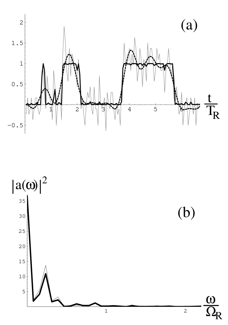
Figure 1: Quantum jump regime with fuzziness $f=0.07$ and parameters $\Delta p=-0.3\,,p_{0}=0.5\,,\tau=0.002T_{R}\,,N=25$. In Figure (a) black represents the $|c_{2}|^{2}$-curve, gray the measurement readout $G_{2}(t)$ and the dashed curve is obtained from the $G_{2}$-curve by noise reduction. On the time axis multiples of the Rabi period $T_{R}$ are indicated. Figure (b) shows the power spectra of the $|c_{2}|^{2}$-curve (black) and the measurement readout (gray). The frequency $\omega$ is given in units of the Rabi period $\Omega_{R}$. Both spectra agree very well.

We discuss the three regimes by considering one typical example for each regime. The characteristic traits can be read off from Figs. 1– 3. In all three cases we have chosen $\tau=0.002T_{R}$ and $N=25$, so that condition (45) is fulfilled. Figs. 1a– 3a show as function of $t/T_{R}$

• the $|c_{2}|^{2}$-curve of the state motion (black),

• the $G_{2}$-curve representing the measurement readout (gray) and

• the processed $G_{2}$-curve obtained after noise reduction (dashed).

The noise reduction is sketched in Appendix C. The related Figs. 1b– 3b show the respective Fourier spectra gained by discrete Fourier transform of the $|c_{2}|^{2}$-curve (black) and the measurement readout $G_{2}$ (grey). The peaks at $k=0$ are caused by the non-vanishing average value of the curves. In the three regimes we find characteristically different results:

5.1 Quantum jump regime

With fuzziness $f=0.07$ there is a rather strong influence of the measurements on the time evolution of the state. The single measurement is still rather sharp and close to a projection measurement. Accordingly, we observe in Fig. 1, that the Rabi oscillations of $|c_{2}|^{2}$, which would appear in the absence of the measurements are completely destroyed. The $|c_{2}|^{2}$-curve (black) shows jumps between extended periods with values approximately equal to $0$ or $1$. This means that if the state of the system is close to an eigenstate $|1\rangle$ or $|2\rangle$, it has a high probability to stay there. The $G_{2}$-curve of the measurement readout (gray) reflects very well the $|c_{2}|^{2}$-curve of the state. The peaks of the $|c_{2}|^{2}$-curve pointing upwards and downwards follow the direction of the corresponding peaks of the $G_{2}$-curve. The processed $G_{2}$-curve (dashed) reflects the quantum jump regime even better. In this regime there is a rather good agreement between the readout and the $|c_{2}|^{2}$-curve, but there is no characteristic indication of the undisturbed dynamics. The Fourier spectra show a very good correlation, as can be seen in Fig. 1b.

5.2 Rabi regime

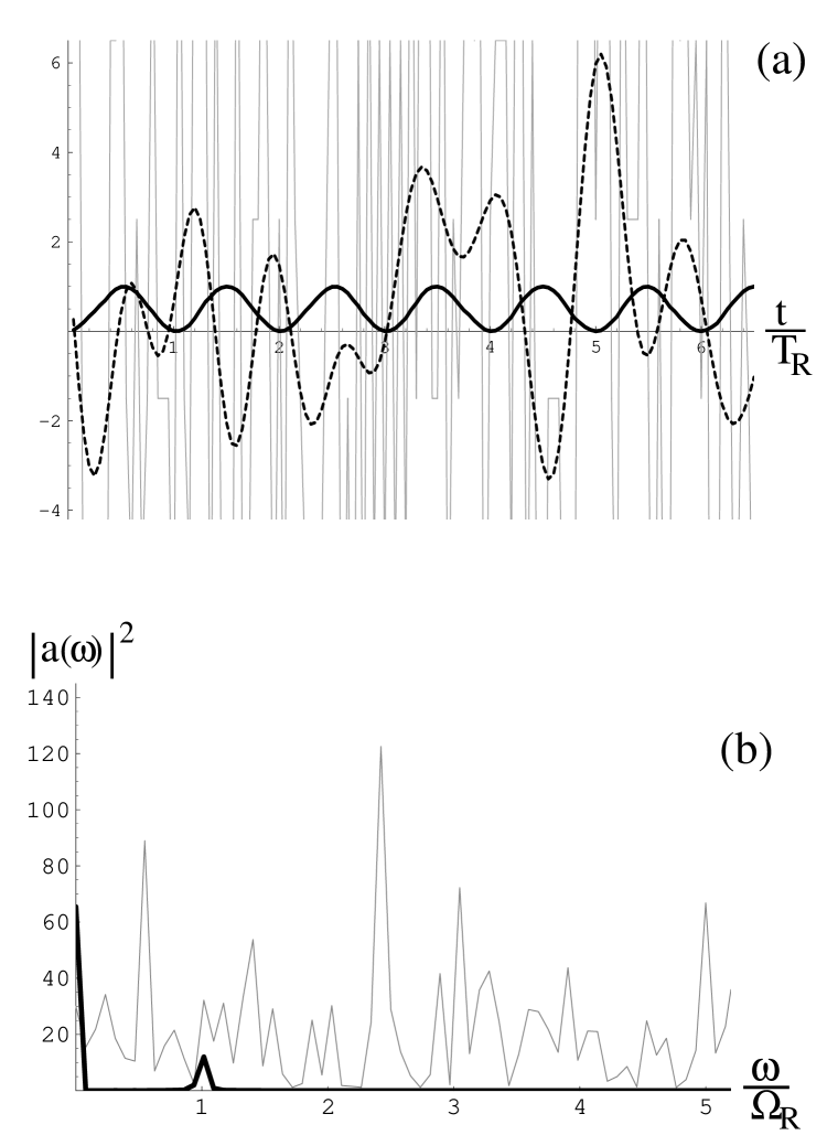
Figure 2: Rabi regime with fuzziness $f=62.8$ and $\Delta p=0.01\,,p_{0}=0.5\,,\tau=0.002T_{R}\,,N=25$. In Figure (a) the numerically obtained $|c_{2}|^{2}$-curve (black) agrees with the undisturbed Rabi oscillations. On the other hand $|c_{2}(t)|^{2}$ is neither significantly correlated with the measurement readout ($G_{2}$-curve, plotted in gray) nor with the processed $G_{2}$-curve (dashed) obtained from the readout by noise reduction. Fig. (b) displays the power spectrum of $|c_{2}(t)|^{2}$ (black) and the power spectrum of the measurement readout (gray). For graphical reasons the power spectrum of the measurement readout has been multiplied by a factor of $1/5$. Both spectra are not correlated.

The other extreme can be found in the Rabi regime. We have chosen a high fuzziness $f=63$. The single measurements are so unsharp and their influence on the motion of the state so weak, that the Rabi oscillations remain nearly undisturbed. This can be seen from the $|c_{2}|^{2}$-curve (black) in Fig. 2a. In contrast to this the $G_{2}$-curve of the measurement readout (grey) is very fuzzy. The single measurement results lie far away from the interval $[0,1]$. The processed $G_{2}$-curve (dashed) shows also no correlation, neither in phase nor amplitude with the $|c_{2}|^{2}$-curve. Turning to the Fourier spectra (Fig. 2b), we see that the Rabi frequency of the $|c_{2}|^{2}$-curve (black) is represented well. On the other hand, no frequency can be attributed to the measurement readout (gray curve). In this regime the measurement readout does not allow a conclusion on the motion of the state as represented by the $|c_{2}|^{2}$-curve.

5.3 Intermediate regime

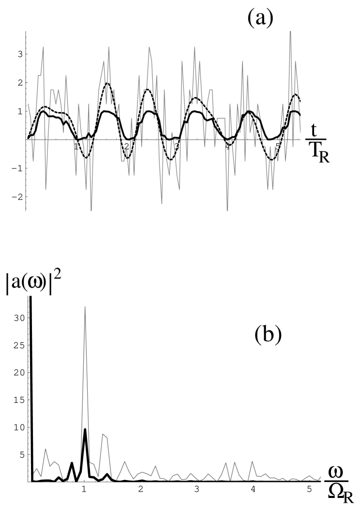
Figure 3: Intermediate regime with fuzziness $f=0.98$ and $\Delta p=0.08$, $p_{0}=0.5$, $\tau=0.002T_{R}$, $N=25$. Fig. (a): There is a high correlation between the $|c_{2}|^{2}$-curve (black) and the measurement readout $G_{2}(t)$ (gray) leading to a very good correlation after the noice of the readout has been reduced (dashed curve). The $|c_{2}|^{2}$-curve indicates that the motion of the state has been disturbed by the measurement. But the Rabi oscillations are still recognizable. Fig. (b): The main peak of the power spectrum of the $|c_{2}|^{2}$-curve (black) coincides with the main peak of the power spectrum of the $G_{2}$-curve and indicates approximately the Rabi frequency $\Omega_{R}$ of the undisturbed motion.

Finally we turn with a fuzziness of $f=0.98$ and $|\Delta p|=0.08$ to a parameter choice, which leads to representative curves for the intermediate regime. According to the Fourier spectrum (black) in Fig. 3b the $|c_{2}|^{2}$-curve is dominated by one frequency, which differs only little from the Rabi frequency $T_{R}$. In this regime the $|c_{2}|^{2}$-curve, which would characterize the state motion if no measurement were performed, is not much modified. The important point is that now the $G_{2}$-curve of the measurement readout (grey) shows a correlation with the $|c_{2}|^{2}$-curve regarding the phase: if the $|c_{2}|^{2}$-curve has a maximum, the $G_{2}$-curve is in the upper domain and for a minimum correspondingly. Regarding the Fourier spectrum of the measurement readout (grey curve in Fig. 3b), there is still a lot of noise, but a clear peak indicates the frequency of the $|c_{2}|^{2}$-curve. The measurement readout follows therefore closely the $|c_{2}|^{2}$-curve of the state motion in phase and frequency. This is even more convincing for the processed $G_{2}$-curve (dashed curve in Fig. 3a).

6 Discussion and conclusions

The normalized state $|\psi(t)\rangle=c_{1}(t)|1\rangle+c_{2}(t)|2\rangle$ of a single two-level system performs oscillations under the influence of a resonant time dependent driving field. It is assumed that there is only one realization of this process available. We ask the question whether it is possible to visualize in real time the evolution of the system as far as it is given by $|c_{2}(t)|^{2}$.

This result can clearly not be obtained by means of standard measurements which result in projections. Generalized measurements, can be discussed by means of positive operator valued measures (POVM). For our goal we restrict to a particular subclass of unsharp measurements, which have a simple structure so that an experimental realization should be possible. The pointer values of this measurements are $+$ and $-$. We perform a sequence of measurements separated in time leading to the pointer readings $+--+-++\ldots$. It can be shown that it is favorable to transform a series of $N$ pointer readings to one point of a measurement readout which is defined as best guess $G_{2}(t)$ for $|c_{2}(t)|^{2}$.

The single unsharp measurement must be weak enough as not to disturb the evolution of the system too much. On the other hand it must not be too weak in order to give information about the state of the system. We determined analytically the domains for the different open parameters such that this ’intermediate’ regime of measurement can be reached. The numerical analysis finally shows that for this intermediate regime the real time visualization of $|c_{2}(t)|^{2}$ can be obtained to a satisfactory amount. The readout $G_{2}(t)$ reflects rather well the resulting $|c_{2}(t)|^{2}$, which itself shows only a slight modification of the undisturbed Rabi oscillations.

Note that above the Rabi frequency of the unitary development was assumed to be known. If this is not the case a feed-back mechanism must be introduced so that after a certain time from the beginning of the measurements a visualization can be reached. This project is subject of future research.

7 Acknowledgment

The authors thank Peter Marzlin for many stimulating discussions. This work has been supported by the Optik Zentrum Konstanz.

Appendix A: How to choose the operations

In order to detect the dynamics of $|c_{2}|^{2}$ we choose measurements with particular operations corresponding to a particular POVM. We justify this choice as follows:

Since our measurement scheme contains consecutive measurements, it is important to consider in which state the system is left after one measurement. We require the operations, which describe the transformation of the state up to a phase factor, to be such that the states $|1\rangle$ and $|2\rangle$ are not changed due to the measurement. Hence these states should be eigenstates of the operations $M_{+}$ and $M_{-}$ in agreement with (3) and (4).

We now address the question why $M_{\pm}$ should be positive operators, thus $u^{+}_{1,2}\,,u^{-}_{1,2}>0$ in (3) and (4) (second requirement of Sect. 2.1). In the context of quantum feedback control one makes use of the fact that the operations may be decomposed into ’modulus’ and ’phase’, in our case:

$$M_{\pm}=U_{\pm}|M_{\pm}|\,,$$ (39)

where $U_{\pm}$ are unitary operators and $|M_{\pm}|:=\sqrt{M^{\dagger}_{\pm}M_{\pm}}$. While the ’modulus’ $|M_{\pm}|$, because of its relation to the effects $E_{\pm}=|M_{\pm}|^{2}$, is connected to the acquisition of information, the unitary operators $U_{\pm}$ represent rather an additional Hamiltonian evolution, not leading to any increase of information about the system (compare Wiseman [17] and Doherty et al. [5]). If thus $U_{\pm}$ cannot be used as a feedback to compensate the influence of $|M_{\pm}|$, it only adds to the disturbance by the measurement and should be set $U_{\pm}=1$ (a global phase factor $\exp(i\varphi_{\pm})$ is always neglected).

That the additional evolution represented by $U_{\pm}$ is indeed obstructive in our case can be made clear as follows. To be diagonalizable the $M_{\pm}$ have to be normal, i.e., $[M^{\dagger}_{\pm},M_{\pm}]=0$ which amounts to $[|M_{\pm}|^{2},U_{\pm}]=0$. Hence $U_{\pm}$ and $|M_{\pm}|$ have a simultaneous basis of eigenvectors, which has to be $|1\rangle$ and $|2\rangle$, because $M_{\pm}$ is required to be diagonal in that basis. Now if $U_{\pm}$ is diagonal with respect to $|1\rangle$ and $|2\rangle$, it can be written as:

$$U_{\pm}=\exp(-\frac{\mbox{i}}{2}\sigma_{z}\theta_{\pm})$$ (40)

for some angle $\theta$ and $\sigma_{z}$ as Pauli operator. In order to illustrate the corresponding different influences on the state motion, we refer to the Bloch sphere. The resonant Rabi oscillations which our system performs in the absence of measurements can be represented by a rotation of the normalized Bloch vector in the y-z-plane (given that the initial state lies in this plane) . The measurement induces a change of the state given by $M_{\pm}$. The contribution due to $|M_{\pm}|$ leads to a jump of the Bloch vector towards one of the ’poles’ on the Bloch sphere at $(0,0,1)$ and at $(0,0,-1)$. The Bloch vector thereby does not leave the plane spanned by the state before the measurement and the z-axis. $U_{\pm}$ on the other hand forces the Bloch vector to leave this plane. As a consequence $U_{\pm}$ cannot compensate the change due to $|M_{\pm}|$ and the influence of $|M_{\pm}|$ is inevitable. Beyond that, a unitary evolution $U_{\pm}\not=1$ disturbs the original Rabi oscillations heavily in a succession of measurements by leading the Bloch vector out of the y-z-plane. Therefore we have to choose $U_{\pm}=1$ in order to disturb the Rabi oscillations by the action of the operations $M_{\pm}$ as little as possible. In an experimental situation with nontrivial unitary transformations $U_{\pm}$ the state change due to $U_{\pm}$ could be compensated by means of feedback (compare Wiseman [17]).

Appendix B: Upper limit for $N$

In this Appendix we describe under which circumstances the concept of the best guess as introduced in Sect. 3 can also be used for N-series with dynamical evolution due to the Hamiltonian in (32) between the single measurements.

Consider a N-series of unsharp measurements which are separated by the unitary evolution according to (32). In the interaction picture the state after the first N-series thus reads:

$$\prod_{k=1}^{N}\,\left(M_{k}\exp\left(-\frac{i}{\hbar}H_{I}\tau\right)\right)|\psi(0)\rangle$$ (41)

with $M_{k}=M_{+},M_{-}$ and $H_{I}:=\hbar\Omega_{R}(|2\rangle\langle 1|+|1\rangle\langle 2|)/2$. We have to discuss for this new situation again the concept of a best guess. If we may commutate unitary evolution and operations representing the change due to the measurement, so that

$$|\psi(\Delta t)\rangle\approx\exp\left(-\frac{i}{\hbar}H_{I}\Delta t\right)\tilde{M}(N_{+},N)|\psi(0)\rangle$$ (42)

with

$$\tilde{M}(N_{+},N):=\sqrt{{N\choose{N_{+}}}}M(N_{+},N)\,,$$ (43)

we are back to the situation described in Section 3.2 and the best guess $G_{2}(t_{m})$ of (30) may be taken as a good candidate to approximate $|c_{2}(t_{m})|^{2}$. The underlying commutators are

$$\left[M_{\pm}\,,\,\exp\left(-\frac{i}{\hbar}H_{I}\tau\right)\right]=\sigma_{y}(u_{1}^{\pm}-u_{2}^{\pm})\sin(\frac{\pi\tau}{T_{R}})\,,$$ (44)

where $\sigma_{y}$ represents the Pauli operator. Although the commutators are small for $\tau/T_{R}\ll 1$, their contribution accumulates and is no longer negligible if the number $N$ of measurements within the N-series is too large.

A lengthy calculation shows that for $N\tau/T_{R}\ll 1$ the term (41) may be approximately written in the form (42), if

$$(N-1)^{2}\ll\frac{\max\{u_{1}^{+},u_{2}^{-}\}}{2\max\{|u_{2}^{+}-u_{1}^{+}|,|u_{2}^{-}-u_{1}^{-}|\}}\frac{T_{R}}{\pi\tau}\,.$$ (45)

Here it was assumed that the matrix elements of the operation $M_{+}$ fulfill $u_{1}^{+}>u_{2}^{+}$. Otherwise the indices $1$ and $2$ in (45) have to be permutated.

Appendix C: Simulation procedure and noise reduction

In this appendix the procedure is described we employed to simulate the measurements of Rabi oscillations on the computer. It is denoted here in form of four instructions:
1) Evolve initial state unitarily according to the undisturbed dynamics of the system; $|\psi(0)\rangle\rightarrow|\psi(\tau)\rangle=\exp\{-\frac{\mbox{i}}{\hbar}H_{I}\tau\}|\psi(0)\rangle\,.$
2) Simulate single unsharp measurement in two steps. First generate a random outcome by a Monte Carlo method according to the probabilities $p_{\pm}=\langle E_{\pm}\rangle_{\psi(\tau)}$. Then change the state depending on the outcome $|\psi(\tau)\rangle\rightarrow M_{\pm}|\psi(\tau)\rangle$.
3) N-series: Carry out instructions 1) and 2) $N$ times, every time replacing the initial state by the state obtained after the previous unsharp measurement. After the N-series record $|c_{2}(t_{1}=N\tau)|^{2}$ of the current state and the measurement readout, i.e., the best guess $G_{2}(t_{1})$ for $|c_{2}(t_{1})|^{2}$. The best guess is calculated from the number of $+$-results (c.f. equation (30)).
4) Simulate $M$ times an N-series of unsharp measurements, always inserting as initial state the state obtained from the previous N-series. The total record of the simulation will then consist of a sequence of readouts $G_{2}(t_{m})$ and squared components of the state $|c(t_{m})|^{2}$ with $t_{m}=m\Delta t\,,m=1...M$.

The readouts from the simulated measurements can now be processed to eliminate noise. We used the following method.
The sequence $(G_{2}(t_{m}))$ is expressed by means of discrete Fourier transform as $G_{2}(t_{m})=\sum_{l=0}^{M-1}\,a(\omega_{l})\exp(i\omega_{l}t_{m})$, with $\omega_{l}=2\pi l/T$. From the power-spectrum ($|a(\omega_{l})|^{2}$) the main peak (if present) is identified with the modified Rabi frequency and the noise is estimated.

The noise is reduced by transforming the Fourier coefficients employing a Wiener filter $\phi_{l}$ [18]: $a(\omega_{l})\rightarrow a(\omega_{l})\phi_{l}$. Further noise reduction is achieved by omitting higher frequencies in the Fourier series which cannot be related to the original Rabi oscillation. We truncated the Fourier series after the $2l$-th term, where $\omega_{l}$ is the frequency of the main peak of the power spectrum.

The resulting filtered and truncated Fourier series leads to a new sequence of best guesses $(G_{2}(t_{m}))$ in the text referred to as ’processed measurement readout’ or ’processed $G_{2}$-curve’.

References

- [1] E. B. Davies, Quantum Theory of Open Systems, (Academic Press, London, 1976); C. Helstrom, Quantum Detection and Estimation Theory (Academic Press, New York, 1976); A. Holevo, Probabilistic and Statistical Aspects of Quantum Theory (North-Holland, Amsterdam, 1982); K. Kraus, States, Effects and Operations, (Lecture Notes in Physics 190) (Berlin, Springer, 1983); G. Ludwig, Foundations of Quantum Mechanics, Vol I (Springer, Berlin, 1983). E. Prugovec̆ki, Stochastic Quantum Mechanics and Quantum Space-time (Reidel, Dordrecht, 1984).
- [2] P. Bush, M. Grabowski and P. J. Lahti Operational Quantum Physics (Springer Verlag, Heidelberg, 1995).
- [3] M. W. de Muynck and A. J. A. Hendrikx,The Haroche-Ramsey experiment as a generalized measurement, e-print quant-ph/0003043.
- [4] H. Martens and W.M. de Muynck, Found. of Phys. 8,255,(1990).
- [5] A. C. Doherty, K. Jacobs and G. Jungman, Information, disturbance and Hamiltonian quantum feedback control, e-print quant-ph/0006013.
- [6] J. Audretsch and M. B. Mensky, Phys. Rev. A 56, 44 (1997).
- [7] M. B. Mensky, Phys. Rev. D 20, 384 (1979); A. Barchielli, L. Lanz and G. M. Prosperi, Il Nuovo Cimento 72 B, 79 (1982); L. Diósi, Phys. Lett. A 129, 419 (1988)
- [8] J.Audretsch, M.Mensky and V.Namiot, Phys. Lett. A237, 1 (1997).
- [9] J. Audretsch, Th. Konrad and M. Mensky, Approximate real time visualization of a Rabi transition by means of continuous fuzzy measurement, to appear in GRG, e-print quant-ph/9907026.
- [10] A.N.Korotkov, Output spectrum of a detector measuring quantum oscillations, e-print cond-mat/0003225.
- [11] H-S. Goan, G. J. Milburn, H. M. Wiseman and H. B. Sun Continuous quantum measurement of two coupled quantum dots using a quantum point contact: A quantum trajectory approach, e-print cond-mat/0006333.
- [12] J. Audretsch, M. B. Mensky Realization scheme for continuous fuzzy measurement of energy and the monitoring of a quantum transition, e-print quant-ph/9808062.
- [13] J. Audretsch, Th. Konrad and A. Scherer, Quantum optical weak measurements can visualize photon dynamics in real time, e-print quant-ph/0012060.
- [14] M.A.Nielsen and I.L.Chuang, Quantum Computation and Quantum Information, (Cambridge University Press, Cambridge, 2000)
- [15] D.Sondermann, Die Iteration nichtzerstörender quantenmechanischer Messungen, (ph.d.-thesis University of Göttingen (Germany), 1998).
- [16] M. Brune, S. Haroche, V. Lefevre, J.M. Raimond and N. Zagury, Phys. Rev. Lett., 65, 976 (1990).
- [17] H. M. Wiseman, Phys. Rev. A 51, 2459 (1995).
- [18] W. H. Press et al., Numerical Recipes in C: the Art of Scientific Computing (Cambridge Univ. Press, Cambridge 1992).