1 Introduction

More than 50 years ago, Casimir predicted that two parallel conducting plates attract each other in vacuum [1]. The attraction is the result of a modification of the electromagnetic modes between the plates caused by the conducting boundaries. The magnitude of this force per unit area between parallel plates, at separation $d$, is:

$${F\rm(\mit d\rm)\over\mit A}\rm=-{{\mit\pi}^{\rm 2}\mit\hbar c\over\rm 240{\mit d}^{\rm 4}}$$ (1)

Despite its implications in areas as diverse as cosmology, Rydberg atom spectroscopy, particle physics, and quantum field theory (see [2, 3] for reviews), quantitative experimental verification did not appear until very recently, when Lamoreaux investigated this force in the range 0.6-6 $\mu$m using a torsion pendulum [4], and Mohideen and Roy used an atomic force microscope (AFM) for studies in the 0.1-0.6 $\mu$m regime [5, 6]. The agreement with theory was claimed to be 5% and 1% in these experiments, respectively, but surface roughness, the use of multi-layer structures, and uncertainty regarding the absolute surface separation complicate the analysis in both cases. The experimental setups in these experiments were sphere-flat configurations (which is mathematically equivalent to the crossed-cylinder geometry used in this study). For these cases, the proximity force theorem [7] (or “Derjaguin approximation” [8]) can be used to transform the result for parallel flats, yielding instead for a sphere and a flat (or two crossed cylinders):

$${\mit F\rm(\mit D\rm)}\rm=-{{\mit\pi}^{\rm 3}\mit R\hbar c\over\rm 360{\mit D}^{\rm 3}}$$ (2)

where ${\mit D}$ is the closest separation between the bodies, and ${\mit R}$ is the radius of the sphere for the sphere-flat geometry, whereas for crossed cylinders $R\rm=\sqrt{{\mit R}_{\rm 1}{\mit R}_{\rm 2}}$, where ${\mit R}_{\rm 1}$ and ${\mit R}_{\rm 2}$ are the radii of the cylinders. The Casimir result holds for two smooth and perfectly conducting bodies interacting in vacuum at zero temperature, and considerable effort has been devoted to the derivation of corrections to Eq. (2) for non-ideal experimental conditions.

The correction for finite temperature has different functional forms depending on the value of the parameter $t=\mit k_{\rm B}TD/\hbar c$. For the temperatures and separations considered here, $t$ $\stackrel{{\scriptstyle\scriptstyle<}}{{\scriptstyle\sim}}$ 0.01, which is in the low temperature regime [9, 10]. The relative magnitude of this correction is less than $10^{-4}$ in the range 20-100 nm, and is apparently of little importance.

The deviations from the Casimir result due to finite conductivity have been estimated using a plasma model of the metal with dielectric function $\mit\varepsilon(\omega)\rm=1-\mit\omega_{p}^{\rm 2}/\omega^{2}$, where $\omega_{p}$ is the bulk plasma frequency. The correction has the form of a series expansion in terms of $\lambda_{p}/D$ [10, 4, 11], and has been determined at least to the fourth order [12]. At small separations, where the wavelengths of the lowest possible intersurface modes approach the plasma wavelength, the correction for finite conductivity based on the plasma model is no longer valid. Lamoreaux [13] calculated the interaction with Lifshitz teory [14] instead, using spectroscopic data. This avoids using the plasma model conductivity correction, but instead introduces the difficulty of determining the frequency dependence of the permittivity of the metal over a wide frequency range. In this report, where the separation range is $<\omega_{p}$, a similar method is used.

In the roughness correction by Klimchitskaya [15], the corrugation amplitude $\mit{A}_{r}$ is chosen such that the deviation of the surface shape from the ideally smooth is described by $\mit z=A_{r}f_{r}(x,y)$, where $\rm max\left|{\mit f_{r}(x,y)}\right|=1$. Thus, $\mit{A}_{r}$ should be taken as half the maximum peak-to-trough roughness over the surface, and assuming a random roughness distribution, the resulting correction is to second order:

$${{\mit F}^{R}\left({D}\right)}={F}\left({D}\right)\left({1+6{\left({{{\mit A}_{r}\over D}}\right)}^{\rm 2}}\right)$$ (3)

Again, higher order contributions have been calculated for some experimental conditions [16].

For further investigations of the Casimir force and related phenomena, improvements not only of the corrections, but also of the experimental procedures are required to obtain accurate results. This report describes the implementation of a surface preparation procedure resulting in macroscopic metal surfaces with arbitrary thickness, whose roughness is about one order of magnitude smaller than reported in previous experiments. The applicability of such surfaces to force measurements is demonstrated by measurements of the Casimir force at separations down to 20 nm.

2 Numerical procedure

The interaction between the metal surfaces were calculated as follows: For two gold plates with dielectric function $\varepsilon_{1}$, covered with hydrocarbon layers ($\varepsilon_{2}$, the purpose of these are explained further down) of thickness $a$, interacting across air (for which we assume $\varepsilon_{3}=1$), the free energy of interaction per area at a separation $d$ is given by [17, 18]:

$$F\rm(\mit d\rm,\mit T\rm)={{\mit k}_{B}\mit T\over\rm 8\mit\pi{d}^{\rm 2}}\sum_{\mit n\rm=0}^{\infty}{{}^{\prime}}\mit I\rm({\mit\xi}_{\mit n}\rm,\mit d\rm)\rm,\hskip 14.22636pt\mit\xi_{n}={{\rm 2}\pi nk_{\rm B}T\over\hbar}$$ (4)

where the prime on the summation means that the term $n=0$ should be halved. The separation $d$ is taken to be zero where the hydrocarbon layers contact each other, see Figure 1. Further,

$$I\rm({\mit\xi}_{\mit n}\rm,\mit d\rm)={\left({{2{\mit\xi}_{\mit n}\mit d\over\mit c}}\right)}^{\rm 2}\int_{1}^{\infty}\rm\Bigl{\{}\ln\left({1-{\left({{\overline{\rm\Delta}}_{\rm 31}}\right)}^{2}\exp{\left(-{2\mit p{\xi}_{n}d\over\mit c}\right)}}\right)\rm$$

$$\mbox{}\rm+\ln\left({1-{\left({{\rm\Delta}_{\rm 31}}\right)}^{2}\exp{\left(-{2\mit p{\xi}_{n}d\over\mit c}\right)}}\right)\Bigr{\}}\mit p\rm d\mit p$$

(5)

where

$${\overline{\rm\Delta}}_{\rm 31}={{\overline{\rm\Delta}}_{\rm 32}+{\overline{\rm\Delta}}_{\rm 21}\exp\left({-{2\mit{\xi}_{n}as_{\rm 2}\over\mit c}}\right)\over 1+{\overline{\rm\Delta}}_{\rm 32}{\overline{\rm\Delta}}_{\rm 21}\exp\left({-{2\mit{\xi}_{n}as_{\rm 2}\over\mit c}}\right)}$$

(similarly for ${\rm\Delta}_{\rm 31}$). For any two adjacent layers $i$ and $j$

$${\overline{\Delta}}_{ij}={{s}_{j}{\varepsilon}_{i}-p{\varepsilon}_{j}\over{s}_{j}\varepsilon_{i}+p\varepsilon_{j}}\rm,\hskip 5.69054pt\mit{\rm\Delta}_{ij}={s_{j}-p\over s_{j}+p}\rm,\hskip 5.69054pt\mit s_{j}=\sqrt{p^{\rm 2}-{\rm 1}+\varepsilon_{j}}$$

where $\varepsilon_{i}=\varepsilon_{i}\rm(\mit i\xi\rm)$. The dielectric function has a real and an imaginary component, $\varepsilon\rm(\mit\omega\rm)=\mit\varepsilon\rm^{\prime}(\mit\omega\rm)+\mit i\varepsilon\rm^{\prime\prime}(\mit\omega\rm)$. For a given frequency $\rm\varepsilon^{\prime}+\mit i\varepsilon\rm^{\prime\prime}={\mit n}^{\rm 2}-{\mit k}^{\rm 2}+\mit i\rm 2\mit nk$, but only the imaginary part of the dielectric function is required to calculate $\varepsilon\rm(\mit i\xi\rm)$ along the imaginary axis, using the Kramers-Kronig relationship:

$$\varepsilon\rm(\mit i\xi\rm)=1+{2\over\mit\pi}\int_{\rm 0}^{\infty}{\mit x\varepsilon\rm^{\prime\prime}(\mit x\rm)\over{\mit x}^{\rm 2}+{\mit\xi}^{\rm 2}}\rm d\mit x$$ (6)

Tabulated spectroscopic data ($n$ and $k$) for gold [19] was used to calculate $\varepsilon\rm(\mit i\xi\rm)$ using (6) for each frequency $\xi_{n}$. In the low-frequency regime, the dielectric function was extrapolated using a Drude model:

$$\varepsilon\rm(\mit i\xi\rm)=1+{{\mit\omega}_{\mit p}^{\rm 2}\over\rm(\mit\xi^{\rm 2}\rm+\mit\gamma\xi\rm)}$$ (7)

The plasma frequency $\omega_{p}$ = 1.4 $\times 10^{16}$ and the relaxation parameter $\gamma$ = 5.3 $\times 10^{13}$ were obtained as described in [20]. The optical properties of the hydrocarbon layer were modelled with a single oscillator [17]:

$$\varepsilon\rm(\mit i\xi\rm)=1+{(\mit n^{\rm 2}\rm-1)\over 1+(\mit\xi\rm/{\mit\omega}_{\rm UV})}$$ (8)

where $n=1.5$ and $\omega_{\rm UV}=3.0\times 10^{15}$ for a solid hydrocarbon [21]. Beyond the plasma frequency ($\omega_{p}^{\rm 2}=\mit Ne^{\rm 2}/\varepsilon_{\rm 0}m_{e}$) the plasma model was used. The total interaction does not depend critically on the hydrocarbon layer, and more elaborate models did not produce significantly different results.

For gold and hydrocarbon, $\varepsilon\rm(\mit i\xi\rm)$ was calculated from $10^{14}$ to $10^{19}$ rad/s, by integration of (6) between $10^{12}$ to $10^{21}$ rad/s for each frequency $\xi$. The integral (5) was then evaluated for $p$ between $1$ and $10^{4}$, and the summation in (4) continued until doubling the number of terms resulted in a change of less than 0.01%.

To fit the calculated interaction to the measured data the function

$$\rho=\rm{\left(\mit F_{exp}(d+\delta)-F_{calc}(d)-{\alpha\over d}\rm\right)}^{2}$$ (9)

was minimized with respect to $\delta$ and $\alpha$. The first term on the right hand side is the measured force, where the parameter $\delta$ is the deformation of the surfaces along the symmetry axis, and is used to obtain the true surface separation. The second term is the calculated interaction as described above, corrected for surface roughness to the second order. The last term is the electrostatic force between the surfaces caused by residual potential differences.

3 Experimental procedure

The gold surfaces were prepared by a template-stripping method adapted from Wagner [22]. Thin (10-15 $\mu$m) freshly cleaved mica sheets were cut in $\rm 1\times 1\ {cm}^{2}$ pieces using a hot platinum wire, and a 200 nm gold layer was deposited onto the mica in an ultra-high vacuum evaporator at a rate of 0.5 nm/s, with the evaporation pressure typically at $3\times{10}^{-8}$ Torr (considerably thicker gold layers can be prepared in the same manner with no differences in subsequent preparation steps, the roughness of the final gold surface remains the same). The gold-coated mica pieces were glued (Epo-Tek 301-2, Epoxy Technology) gold-side down onto cylindrical silica discs (R = 10 mm). The day before use, the discs were immersed in tetrahydrofurane until the mica sheet came loose (a few minutes). After drying in a gentle N₂ flow, 50 $\mu$m gold wires were attached to the bare gold using a gold spring clip, whereupon the surfaces were immersed into a 1 mM solution of hexadecanethiol (Fluka, 95%) in ethanol, and incubated overnight. The hexadecanethiol self-assembles into a close-packed crystalline monolayer, with the hydrocarbon chains facing outwards and the thiol covalently attached to the gold substrate [23]. This layer prevents contaminants from the laboratory atmosphere to adsorb onto the surface [24], and so serves to keep the surface well-defined, which is necessary for estimating surface deformation in the force measurements. It also prevents cold welding of clean gold layers in contact, which would damage the surfaces upon separation. The thickness of each thiolate layer is approximately 2.1 nm [25]. After removal from the thiol solution, the samples were sonicated in ethanol to remove physisorbed thiols. The surfaces were then mounted in a crossed-cylinder configuration in the force measuring device, and the wires from the two surfaces were connected with a gold clip, providing an all-gold conducting path between the surfaces (in such a way that the movement of one surface is not transmitted to the other surface through the wire).

The surface roughness was measured with an AFM (Nanoscope III, Digital Instruments) in tapping mode. The roughness parameters are as measured over $\rm 1\times 1\ \mu{m}^{2}$, and evaluated using the software supplied with the instrument.

The contact angles with water were determined by slowly expanding a droplet on a flat template-stripped hydrocarbon covered surface, and determining the angle formed between the water droplet and the substrate with a microscope goniometer (Rame-Hart NRL 100).

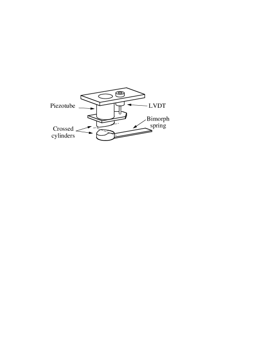
Figure 2: Simplified view of the force measuring device. The position of the upper surface is controlled with a motorized stage (not in figure) and a piezoelectric tube, while the response of the lower is detected with the bimorph transducer, acting as the measuring spring. The LVDT is used to monitor the non-linear expansion of the piezotube. The radius of curvature of the cylindrical surfaces is 10 mm.

The force measurement device (Figure 2) works in a manner similar to the AFM, but is designed for measurements between macroscopic surfaces [26]. One surface is mounted onto a piezoelectric tube, whose position can be adjusted with a motorised translation stage to within $\pm$ 50 nm. A linearly variable displacement transducer (LVDT) is mounted in parallel with the piezo to measure the tube expansion, in order to eliminate piezotube hysteresis in the subsequent data analysis. The other surface is mounted onto a piezoelectric bimorph deflection sensor [27], acting as a single cantilever spring, and the charge produced by the bimorph upon deflection is detected with an electrometer amplifier. A force-distance profile is acquired by moving the surfaces towards each other at a constant rate from a separation $<$ 3 $\mu$m, using the piezotube. When the surfaces contact each other, the surfaces are moved a further 200-300 nm together while being in contact (and the expansion of the piezotube is directly transmitted to the bimorph), before they are separated again. The average approach rate was approximately 80 nm/s. The distance resolution was $\sim 0.1$ nm, and the force resolution $\sim$ 10 nN. Data is presented as equivalent free energy of interaction, i.e. force normalised with 2$\pi\times$radius (F/$2\pi$R); the normalised force resolution is $\sim$ 0.1 $\mu$N/m (or $\mu$J/m²). The force profiles were averaged by arranging the force-distance data pairs from five individual approaches into a single column, sorting the data by distance order and calculating a running average. All experiments were performed in air at 25 $\pm$ 1 ^∘C, and the relative humidity during the experiments was $\leq$ 60%. A set of external caliper gauges with a precision of $\pm 0.05$ mm were used to determine the radii of the surfaces after the experiments. The relatively stiff mica templates used to fix the low viscosity glue in the preparation step, ensure that the deviations of the local radii from the macroscopic radii are small. The studied separation range was determined by the force measurement device: the force resolution limit approaches the magnitude of the calculated result at separations beyond 100 nm, and at about 20 nm, the gradient of the force is comparable to the stiffness of the measuring spring, and the surfaces “jump” into contact.

4 Results

Surface preparation

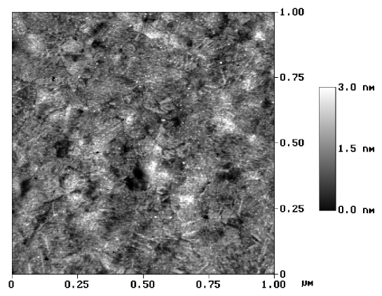
Figure 3: Atomic force microscope image showing the structure of the template-stripped gold surfaces. The peak-to-trough roughness over $\rm 1\times 1\ \mu{m}^{2}$ areas are 3-4 nm, the corresponding rms roughnesses 0.3-0.4 nm.

AFM investigation of the template-stripped gold surfaces reveal peak-to-trough roughness of 3-4 nm, with corresponding root-mean-square (rms) roughness in the 0.3-0.4 nm range (see Figure 3). A significant contribution to the peak-to-trough value comes from a sparse population of pinholes in the layer, probably resulting from insufficient annealing or heterogeneous growth of the gold layer during the initial stages of the evaporation. Comparing the results with those of Wagner [22], it appears that annealing the films after evaporation might yield a further reduction of the roughness. Compared to the 3 nm rms roughness amplitude reported by Roy in a recent report using a smooth metal coating [6], the template-stripping method yields a reduction of the roughness with almost one order of magnitude. With this roughness amplitude, however, the second order roughness correction is still $\sim$ 20% at 20 nm, and the calculated Lifshitz result must be corrected accordingly.

The contact angles with water after adsorption of the thiolates was 110$\pm$2^∘, indicating that the surfaces expose a dense hydrocarbon layer.

Force measurements

A force-distance profile for a single approach is shown in Figure 4. There appears to be no significant electrostatic interaction at large separations, which is also confirmed by the result of the fitting procedure (see further down). However, the used method provides only indirect determination of the separation between the surfaces, and the distance scale has to be corrected for deformation of the surfaces caused by attractive forces when they are in contact. The relatively soft glue used to support the gold layer causes the surfaces to deform substantially, but the layered structure of the surface makes direct application of continuum theories for surface deformation questionable [28]. The central displacement $\delta$, i.e. the total compression of the two surfaces along the symmetry axis has been calculated using finite element analysis for the silica-glue-gold system under consideration, and was found to be 18-20 nm for surfaces with the glue thicknesses used here [29]. This implies that the measured force profiles should be shifted 18-20 nm towards shorter separations.

Figure 5 shows two force profiles calculated as averages of five different approaches in two independent experiments. Fitting the averaged data to the Lifshitz result using (9) yields a total compression $\delta$ of 9 and 12 nm, respectively, in moderate agreement with the numerical result. However, the calculated value of the compression corresponds to the contact of ideally smooth surfaces, while the finite roughness of the real surfaces reduces the adhesion (and the central displacement), and the calculated value must be used as an upper bound to the actual central displacement. Taking this into consideration, the deviations are perfectly reasonable.

The parameter $\alpha$ measuring the electrostatic contribution to the force is $<1.3\times 10^{-23}$ Nm for both data sets, which results in an electrostatic force of the order of the instrument resolution at the shortest separation, and it is concluded that this contribution to the total interaction can be ignored (replacing the 1/$d$ term with a 1/$d^{\rm 2}$ term, taking patch charges into account, does not improve the fit).

The absence of charges on the dielectric hydrocarbon surface might be surprising, but is probably a result of the natural humidity in the air surrounding the surfaces. At the relative humidities (RH) where the experiments were performed ($\leq$ 60%), the amount of water adsorbed from the atmosphere onto the non-polar hydrocarbon layers is small, however. For similar surfaces the water coverage at 100% RH has been determined to 0.8 monolayers [30]. For solid polyethylene with higher affinity to water (contact angle $\theta$ = 88^∘), water layers of the order of 0.1 nm at 60% RH have been reported [31], while a surface conductivity study arrived at a 3 monolayer water thickness at 100% RH for a surface with $\theta$ = 104^∘ [32]. Thus, assuming a 0.1 nm thick water layer on the surfaces appears to be a pessimistic estimate, and the effect on the interaction of such a layer was calculated using an oscillator model for water, where a Debye relaxation term in the microwave region is added to damped harmonic oscillators in the IR (5 terms) and UV (6 terms) regions, with parameters as described by Parsegian [33] and Roth [34]:

$$\varepsilon\rm(\mit i\xi\rm)=1+\mit{f\over\rm 1+\mit g\xi}\rm+\mit\sum\nolimits\limits_{j}{{f}_{j}\over{\omega}_{j}^{\rm 2}+{\xi}^{\rm 2}+{g}_{j}\xi}$$ (10)

For equivalent separations between the solid surfaces, the effect of such a water layer corresponds to an increase in the calculated interaction of $\approx$ 1% at 20 nm. Considering the assumption of a rather thick water layer, the error introduced by neglecting this in the calculations is therefore concluded to be small.

After fitting the data, the total rms force deviation is $<$ 1% of the force at 20 nm. The small differences between the two experimental data sets in Figure 5 after fitting indicate that the precision (repeatability) in the measurements is good, in fact as good as the agreement with the calculated interaction (the accuracy), using the same measure as above.

5 Discussion

The precision of the measurement

Although the rms deviation between the experimental and theoretical results is $<$1% at the shortest separation, it appears that this result cannot – for several reasons – be taken as confirmation of the theory at the same level of agreement. First, the Lifshitz calculations based on optical data is insecure in that the optical data is incomplete, and extrapolations have to be made; the potential errors due to the choice of optical models in the extrapolated regimes (and the parameters used to describe them) have been reported recently [20, 35], and to ensure that correct data is used, spectroscopic data should be collected for the very surfaces that are used in the force experiments.

Further, from the series of reports by Mohideen and co-workers [5, 36, 12], it seems that the relative rms error at the shortest separation is too blunt a measure of the agreement between theory and experiment: the first analysis of their experiment in the range 100-900 nm used a method where the Casimir force corrections to second order for conductivity, roughness and for the finite temperature were multiplied together, resulting in an rms deviation (as calculated over the whole interaction range) corresponding to 1% of the force at the shortest separation [5]. This analysis was criticized by Lamoreaux [37], claiming that the agreement must be coincidental, since the corrections for conductivity and roughness were not sufficiently detailed, and that the potential error caused by this might be greater than 50%. Subsequently, a different theory, including the roughness and conductivity corrections to fourth order (and some “cross-terms” as well), and using a more elaborate quantitative description of the surface roughness, was used to produce a similar 1% relative precision at the shortest separation for the same data [12]. Thus, since it is emphasized in [5, 36, 12] that no adjustable parameters were used, it seems that a 1% rms agreement at the shortest separation allows for erroneous models to fit the data, and should perhaps be considered an inappropriate criterion for agreement between theory and experiment.

One reason for this is that the rms error calculated as $\sigma=\sqrt{\sum(F_{exp}-F_{calc})^{\rm 2}/N}$ is unsuitable for relative error estimates for non-linear functions with wide variations in magnitude; even though the relative error in the measurement can amount to 100% or more at large separations where the magnitude of the measured force approaches the resolution of the instrument, the average of those will be a small absolute error when measured relative to the magnitude of the force at small separations. Averaging further into the region of low magnitude will continually decrease the rms error. For the data presented in Figure 5, the rms error decreases if the spearation range used for the calculation is increased, as is clear from Figure 6. The rms deviation relative to the force at the shortest separation is 0.48% if the deviation is computed from 20 to 100 nm, decreasing to 0.36% if the rms error summation is continued to 300 nm instead; indeed a meaningless measure of the accuracy. At approximately 100 nm, the calculated force is of the order of the resolution of the instrument, and beyond this point the accumulated rms error decreases monotonically, even though the relative error in the measurement is steadily increasing, see Figure 7. For a single figure to measure the deviation between theory and experiment, the error at a particular separation is probably better weighted with the magnitude of the force, and the averaging certainly should not continue beyond the point where the magnitude of the calculated interaction approaches the noise level. The rms figures provided in [12] show a similar trend; for deviations measured over 30, 100 and 223 data points (corresponding to separations 80-200, 80-460 and 80-910 nm) the rms error is 1.6, 1.5 and 1.4 pN, respectively.

Whenever the separation between the surfaces is not measured directly (and with high accuracy), the uncertainty in the location of the measured curve along the separation scale will always be a source of error. In the experiments presented here, the deformation of the surfaces is the only remaining fit parameter of significance, but it is not possible to establish with certainty that the central displacement $\delta$ obtained through the fit procedure is correct, which diminishes the strength of the measurement as a test of the Casimir force, and also precludes a quantitative assessment of the agreement between theory and experiment.

To determine the merit of the corrections to the Casimir force, a precise determination of the separation is essential; the corrections for conductivity and roughness are both expansions in 1/$d$, increasing their effect at shorter separations. If there is uncertainty in the separation, the error caused by using the wrong theory is easily obscured by a shift along the separation axis, which corrects for the deviations at small separations where the errors are greatest, while making little difference at larger separations where the force profile is much flatter. If, using the data in Figure 5, the roughness correction is ignored in the calculated force profile, the total rms deviation at the smallest separation is 0.49% for the rms calculated in the range 20-100 nm, provided the experimental data is shifted 3.1 nm along the separation axis. Without shifting the curve, the rms error can be kept $<$1% if averaging is continued to 400 nm. Besides, the data in Figure 5 can be shifted 0.5 nm in either direction, still keeping the rms error $<$1% for averages between 20 and 100 nm.

The ambiguity due to the fact that the rms error is continuously decreasing as it is calculated over larger separations, implies that the relative rms error at the shortest separation is an unsuitable measure of the agreement between theory and experiment, and the 1% level, in particular, is too broad to discriminate the second order roughness correction from no correction at all, even though the magnitude of the forces differ with as much as 20%.

In a similar fashion, the Au/Pd layers covering the Al surfaces used in [5, 6, 12] were ignored in the analysis, but could be accomodated as additional layers with effective permittivity $\varepsilon\approx$ 1.2 without changing the rms error, provided all separations are increased 3 nm [12]. Incidentally, the plasma wavelength used in [5, 36, 12], $\lambda_{p}=$ 100 nm, was taken from [19], which gives “$\sim 15$ eV” as the plasmon energy, corresponding to $\lambda_{p}\approx$ 83 nm. Already this difference causes a $>$3% deviation in the conductivity correction used in [36], where at the same time it is mentioned that “Small changes in $\lambda_{p}$ will not significantly modify $\sigma$.”, which appears to confirm that $\sigma$ is not a very good measure of the accuracy.

The methodological improvement

The principal methodological improvement in this report is the preparation of metal surfaces with reduced surface roughness, though other problems common to this and the experiments discussed hitherto remain: the unknown absolute surface separation, the effect of additional layers, the determination of the permittivity (or finite conductivity correction) of the metals, and the presence of other interactions (principally electrostatic contributions). The suggested procedure does not avoid these problems, but the two first points deserve some attention.

The use of macroscopic surfaces improves accuracy, since the magnitude of the involved forces are greater, but instead entails enhanced surface deformation problems. Any two bodies in contact deform to an extent determined by a balance between the reduction in surface energy and the elastic strain energy caused by the deformation; for the gold-glue-silica system the deformation at surface contact (with zero applied external load) was calculated to be 18-20 nm. If the two crossed cylinders used in the experiments were solid gold (all other things being equal), the calculated deformation would have been 7 nm (see the Appendix for details). Klimchitskaya et al. mention that smoother metal coatings and surfaces with larger radii can be used to improve the precision of the measurements [12], but this will inevitably lead to increased problems with surface deformation. It is a mistake to assume that this is a problem limited to the use of macroscopic surfaces only, but it ought to be a matter of concern also in the analysis of past AFM experiments [5, 6, 12]. If the surfaces are smooth and the interfacial energy of the contact is that of two hydrocarbon surfaces (which is about as low as is practically achievable in air or vacuum), a 200 $\mu$m polystyrene sphere (used in [5, 6]) interacting with a silica plate is compressed $\sim$10 nm upon contact, under zero applied load (see the Appendix for details). Now, roughness decreases this figure since the effective contact area decreases, but on the other hand, the interfacial energy of a clean metal-metal contact might be two orders of magnitude higher than that for two hydrocarbon surfaces. These issues have to be addressed if a proper estimate of the separation uncertainty is to be established.

The hydrocarbon layers described in this report were used both to keep the surfaces well-defined – which is essential for deformation estimation – and to avoid cold welding of the gold layers in contact. Thus, besides producing surfaces with low roughness, the proposed preparation procedure has the added advantages that the surface energy is well defined (and small) by use of the hydrocarbon layer, and that the theoretical treatment of this layer is fairly straightforward.

6 Conclusion

In conclusion, a template-stripping method was used to prepare smooth gold surfaces, with $\leq$0.4 nm rms roughness. The roughness is independent of the thickness of the gold layer, and is about one order of magnitude smaller than surfaces used in previous experiments. These surfaces (covered with a hexadecanethiolate overlayer) were used to measure the Casimir force in air at separations between 20 and 100 nm, a range that has previously been inaccessible due to the roughness of the samples. The results were found to be in good agreement with the Lifshitz prediction for the interaction, once the deformability of the surfaces had been taken into account. The experimental uncertainties, above all the deformation, makes a quantitative assessment of this agreement difficult, however. Using the obtained data, it is also demonstrated that the rms error is a very ambiguous quantitative measure of the agreement between theory and experiment, and in particular that a 1% level is not cogent enough to discriminate the effect of corrections to the Casimir force.

Surface deformation

To calculate the deformation of elastic bodies in contact the models by Johnson et al. [28] (JKR) and Derjaguin et al. [38] (DMT) are the most commonly used. To discriminate the range of applicability of either model, a dimensionless parameter, $\mu$, is used [39]:

$$\mu\rm={\left({{\mit R{\gamma}^{\rm 2}\over{\mit K}^{\rm 2}{\mit D}_{e}^{\rm 3}}}\right)}^{{1/3}}$$ (11)

where $R$ is the radius of interaction as described in the Introduction, $\gamma$ is the interfacial energy of the contact, $K=[(1-\nu_{\rm 1}^{\rm 2})/E_{\rm 1}+(1-\nu_{\rm 2}^{\rm 2})/E_{\rm 2}]^{\rm-1}$ contains two materials constants, the Young’s modulus $E$, and the Poisson ratio $\nu$, for each material. $D_{e}$ is the equilibrium separation between the surfaces in contact, which is difficult to establish, but a few Å is a typical estimate. For $\mu<0.1$, that is for small and/or hard particles, the DMT model is appropriate, while the JKR applies where $\mu>5$, and the interacting bodies are large and/or soft [40]. Most macroscopic surfaces fall into the latter category, and so does the polystyrene spheres used in some recent AFM experiments [5, 6]. For polystyrene spheres with $R=$ 200 $\mu$m, Young’s modulus $3\times 10^{9}$ Pa and Poisson’s ratio 0.33, interacting with a silica plate with $E=8\times 10^{10}$ Pa and $\nu=0.42$, and further assuming an equilibrium surface separation of a few, say, 3 Å, and the interfacial energy of a hydrocarbon-hydrocarbon contact, 0.05 J/m², which is as low as is realistically obtainable, the parameter $\mu\approx$ 12, which is in the JKR regime.

For the present purposes, the JKR result of most interest is the central displacement, $\delta$, i.e. the deformation along the symmetry axis under the externally applied load $F$ (where $F>0$ for compression):

$$\delta\rm={{\mit a}^{\rm 2}\over\mit R}\rm-{\left({2\mit\pi\gamma a\over K}\rm\right)}^{\rm 1/2}$$ (12)

where $a$ is the radius of the contact region, given by

$${a}^{\rm 3}={\mit R\over\mit K}\rm\left({\mit F\rm+3\mit\pi\gamma R\rm+{\left[{6\mit\pi\gamma RF\rm+{\left({3\mit\pi\gamma R}\right)}^{\rm 2}}\right]}^{1/2}}\right)$$ (13)

from which it is clear that the surfaces deform even without externally applied load. The pull-off force, the negative load that has to be applied to separate the surfaces from adhesive contact is:

$$F_{a}=-{\rm 3\over 2}\pi\gamma R$$ (14)

which can be used to determine the interfacial energy of two interacting bodies.

Figure 1: Schematic of the calculated system. The gold layers are assumed semi-infinite, and the thickness $a$ of each hydrocarbon (HC) layer is 2.1 nm. The zero separation ($d$ = 0) refers to the point of contact of the two hydrocarbon layers.

Figure 4: A Force-distance profile for a single approach, the displayed interval comprises approximately 7000 data points.

Figure 5: The solid curves under the arrow represent two independent experiments: each of them is an average of 5 approaches. To compensate for surface deformation, they are shifted towards shorter separations when fitted with the calculated interaction for the gold-hydrocarbon-air system ($\bullet$), where they coincide. The deformations are 9 and 12 nm, respectively, in fair agreement with calculations (see text for details). The dashed line is the Casimir result, Eq. (2).

Figure 6: The accumulated rms error for one of the data sets in Figure 5. The error is calculated over ranges from 20 nm to the separations indicated on the abscissa. The rms error relative to the magnitude of the force at the shortest separation (20 nm) is 1% for the rms error calculated between 10 and 33 nm, decreasing to 0.36% if averaging is continued to 300 nm, even though the relative measurement error increases steadily in this range, see Figure 7.

Figure 7: The magnitude of the relative error for the data set used to calculate the rms error in Figure 6.

References

- [*] Present address: Physical and Theoretical Chemistry Laboratory, Oxford University, South Parks Road, Oxford OX1 3QZ. E-mail: ederth@physchem.ox.ac.uk, fax: +44 (0)1865 275410, tel: +44 (0)1865 275400.
- [1] H. B. G. Casimir, Proc. Kon. Ned. Akad. Wetensch., B 51, 793 (1948).
- [2] V. M. Mostepanenko and N. N. Trunov, Sov. Phys. Usp. 31, 965 (1988).
- [3] P. W. Milonni, The quantum vacuum (Academic Press, Boston, 1994).
- [4] S. K. Lamoreaux, Phys. Rev. Lett. 78, 5 (1997); 81, 5475 (1998).
- [5] U. Mohideen and A. Roy, Phys. Rev. Lett. 81, 4549 (1998).
- [6] A. Roy, C.-Y. Lin, and U. Mohideen, Phys. Rev. D 60, 111101 (1999).
- [7] J. Blocki, J. Randrup, W. J. Swiatecki, and C. F. Tsang, Ann. Phys. (New York) 105, 427 (1977).
- [8] L. R. White, J. Colloid Interface Sci. 95, 286 (1983).
- [9] J. Mehra, Physica 37, 145 (1967).
- [10] J. Schwinger, L. L. DeRaad, and K. A. Milton, Ann. Phys. (New York) 115, 1 (1978).
- [11] V. B. Bezerra, G. L. Klimchitskaya, and C. Romero, Mod. Phys. Lett. 12, 2613 (1997).
- [12] G. L. Klimchitskaya, A. Roy, U. Mohideen, and V. M. Mostepanenko, Phys. Rev. A 60, 3487 (1999).
- [13] S. K. Lamoreaux, Phys. Rev. A 59, 3149 (1999).
- [14] E. M. Lifshitz, Soviet Physics JETP 2, 73 (1956), transl. from J. Exper. Theoret. Phys. USSR 29, 94 (1955).
- [15] G. L. Klimchitskaya and Y. V. Pavlov, Int. J. Mod. Phys. A 11, 3723 (1996).
- [16] M. Bordag, G. L. Klimchitskaya, and V. M. Mostepanenko, Int. J. Mod. Phys. A 10, 2661 (1995).
- [17] J. Mahanty and B. W. Ninham, Dispersion forces (Academic Press, London, 1976).
- [18] V. A. Parsegian and B. W. Ninham, J. Theoret. Biol. 38, 101 (1973).
- [19] Handbook of optical constants of solids, edited by E. D. Palik (Academic Press, Orlando, 1985).
- [20] A. Lambrecht and S. Reynaud, Eur. Phys. J. D 8, 309 (2000), quant-ph/9907105.
- [21] J. N. Israelachvili, Intermolecular and Surface Forces, 2nd ed. (Academic Press, London, 1985).
- [22] P. Wagner, M. Hegner, H.-J. Guntherodt, and G. Semenza, Langmuir 11, 3867 (1995).
- [23] L. H. Dubois and R. G. Nuzzo, Annu. Rev. Phys. Chem. 43, 437 (1992).
- [24] T. Smith, J. Colloid Interface Sci. 75, 51 (1980).
- [25] S. V. Atre, B. Liedberg, and D. L. Allara, Langmuir 11, 3882 (1995).
- [26] J. L. Parker, Prog. Surf. Sci. 47, 205 (1994).
- [27] A. M. Stewart, Meas. Sci. Technol. 6, 114 (1995).
- [28] K. L. Johnson, K. Kendall, and A. D. Roberts, Proc. R. Soc. Lond. A 324, 301 (1971).
- [29] K. L. Johnson, personal communication (the method is described in I. Sridhar, K. L. Johnson, and N. A. Fleck, J. Phys. D: Appl. Phys. 30, 1710 (1997)).
- [30] E. Thomas, Y. Rudich, S. Trakhtenberg, and R. Ussyshkin, J. Geophys. Res. 104, 16053 (1999).
- [31] M. E. Tadros, P. Hu, and A. W. Adamson, J. Colloid Interface Sci. 49, 184 (1974).
- [32] Y. Awakuni and J. H. Calderwood, J. Phys. D: Appl. Phys. 5, 1038 (1972).
- [33] V. A. Parsegian, in Physical chemistry: Enriching topics from colloid and surface science, edited by H. van Olphen and K. J. Mysels (Theorex, La Jolla, Calif., 1975), pp. 27–72.
- [34] C. M. Roth and A. M. Lenhoff, J. Colloid Interface Sci. 179, 637 (1996).
- [35] M. Boström and B. E. Sernelius, Phys. Rev. A 61, 046101 (2000).
- [36] U. Mohideen and A. Roy, Phys. Rev. Lett. 83, 3341 (1999).
- [37] S. K. Lamoreaux, Phys. Rev. Lett. 83, 3340 (1999).
- [38] B. V. Derjaguin, V. M. Muller, and Y. P. Toporov, J. Colloid Interface Sci. 53, 314 (1975).
- [39] J. A. Greenwood, Proc. R. Soc. Lond. A 453, 1277 (1997).
- [40] K. L. Johnson and J. A. Greenwood, J. Colloid Interface Sci. 192, 326 (1997).