A realistic interpretation of the density matrix
II: The non-relativistic case

1 Introduction

In a recent paper [18] we proposed a realistic interpretation of the Schrödinger equation for density matrices, in which the difference between the position arguments of the density matrix is considered as an objective extra space dimension. In the case of a free particle, where the potential $V\left(x\right)$ vanishes, we found solutions which are perfectly localized both in position space and in momentum space; these solutions behave exactly as non-relativistic point-like particles moving at constant speed, with the correct values for all observable quantities. In the general case, where $V\left(x\right)\neq 0$, we pointed out that the natural frequencies of the stationary states in the density matrix representation correspond to the difference between two energy levels in the original quantum system; since the “jumps” between energy levels are observable, while the individual energy levels are not, we trivially deduced that the observable natural frequencies are the same in both representations.

In the first paper the non-relativistic case was treated mainly as an introduction to the relativistic case; in this second paper we will study it in more detail, examining the correspondence between our new representation and the standard representation of non-relativistic quantum mechanics, based on the Schrödinger equation for pure states. In Section 2 we will first summarize the main results of the previous paper, and then we will give a qualitative definition of a quantum trajectory (describing an individual physical system), as opposed to a statistical mixture (describing an ensemble of physical systems); as a consequence, we will reject two basic principles of standard quantum mechanics, namely the superposition principle and the wave function collapse. In Section 3 we will show the results obtained by applying our approach to simple potentials: by examining the linear harmonic oscillator we will shed a new light on the supposed equivalence between energy eigenvectors and stationary states; besides, the delta barrier potential will provide a semi-classical explanation of the tunnel effect, in which an essential feature is the introduction of internal degrees of freedom even for spinless particles. Finally in Section 4 we will present our conclusions.

2 The density matrix representation and the superposition principle

The standard quantum description of a non-relativistic particle moving in one space dimension is based on a wave function $\psi\left(x\right)$, whose time evolution is given by the Schrödinger equation:

$$i\hbar\frac{\partial\psi}{\partial t}=\textrm{H}\,\psi=-\frac{\hbar^{2}}{2m}\frac{\partial^{2}\psi}{\partial x^{2}}+V\!\left(x\right)\psi$$ (1)

We will refer to equation (1) as to the Schrödinger equation for pure states. The time evolution generated by (1) belongs to the group of unitary transformations; a new representation of this group, the density matrix representation, is obtained by means of the fundamental relation

$$\varphi\left(x,y\right)=\psi\left(x\right)\psi^{*}\left(y\right)$$ (2)

If we apply an arbitrary unitary transformation to the pure state $\psi\left(x\right)$, the relation (2) enables us to obtain the same transformation in the density matrix representation. Specifically, if we consider the hamiltonian operator H, the momentum operator P and the position operator Q as generators respectively of time translations, space translations and momentum translations, we easily obtain the following expressions for the same generators in the new representation:

$$\textrm{H}\,\varphi = -\frac{\hbar^{2}}{2m}\left(\frac{\partial^{2}\varphi}{\partial x^{2}}-\frac{\partial^{2}\varphi}{\partial y^{2}}\right)+\left[V\!\left(x\right)-V\!\left(y\right)\right]\varphi$$

$$\textrm{Q}\,\varphi = \left(x-y\right)\varphi$$ (3)

$$\textrm{P}\varphi = -i\hbar\left(\frac{\partial\varphi}{\partial x}+\frac{\partial\varphi}{\partial y}\right)$$

The time evolution in the density matrix representation is then simply

$$i\hbar\frac{\partial\varphi}{\partial t}=-\frac{\hbar^{2}}{2m}\left(\frac{\partial^{2}\varphi}{\partial x^{2}}-\frac{\partial^{2}\varphi}{\partial y^{2}}\right)+\left[V\!\left(x\right)-V\!\left(y\right)\right]\varphi$$ (4)

In the usual interpretation, equation (4) describes the time evolution of mixed states, and therefore its solutions have only a statistical meaning: they are simply useful tools for computing probability amplitudes and expectation values. On the contrary, in our approach the solutions of equation (4) are considered as real objective fields describing individual physical systems. To avoid misunderstandings, in the rest of this paper we will use the expression “density matrix” when we mean the usual statistical interpretation and we will use the new expression “quantum matrix” when we mean a real objective field.

A quantum matrix $\varphi\left(x,y\right)$ depends upon two position coordinates $x$ and $y$; if we want to consider $\varphi\left(x,y\right)$ as a real objective field then we must introduce an objective extra space dimension. Therefore, we will define a new pair of position coordinates

$$x_{S}=\frac{1}{2}\left(x+y\right)\qquad\qquad\qquad x_{D}=x-y$$ (5)

and we will interpret $x_{S}$ as the “physical” position coordinate, while $x_{D}$ will be an “auxiliary” position coordinate, having observable effects only around the point $x_{D}=0$; both $x_{S}$ and $x_{D}$, however, will be considered as objective position coordinates (note that in the definition of $x_{D}$ we have inverted the sign convention with respect to our first paper [18]). In the rest of this paper we will write loosely $\varphi\left(x,y\right)$ or $\varphi\left(x_{S},x_{D}\right)$, meaning the same field expressed in two different coordinate systems.

The transition from position space to momentum space is obtained by means of the two-dimensional Fourier transform:

$$\Phi\left(k_{x},k_{y}\right)=\frac{1}{2\pi}\int\!\int{\varphi\left(x,y\right)e^{-ik_{x}\!x+ik_{y}\!y}\mathrm{d}x\,\mathrm{d}y}$$ (6)

Again we define a new pair of momentum coordinates:

$$k_{S}=\frac{1}{2}\left(k_{x}+k_{y}\right)\qquad\qquad\qquad k_{D}=k_{x}-k_{y}$$ (7)

and again $k_{S}$ will be the “physical” momentum coordinate, while $k_{D}$ will be an “auxiliary” momentum coordinate, having observable effects only around the point $k_{D}=0$.

Since we have two position coordinates and two momentum coordinates, we naturally can define two position operators and two momentum operators. The operators already defined in (3) may be rewritten as:

$$\textrm{Q}_{D}\,\varphi=x_{D}\,\varphi\qquad\qquad\qquad\quad\textrm{P}\!_{D}\,\varphi=-i\hbar\frac{\partial\varphi}{\partial x_{S}}\quad$$ (8)

In addition, we introduce the new operators $\textrm{Q}_{S}$ and $\textrm{P}\!_{S}$ by means of the following definition:

$$\textrm{Q}_{S}\,\varphi=x_{S}\,\varphi\qquad\qquad\qquad\quad\textrm{P}\!_{S}\,\varphi=-i\hbar\frac{\partial\varphi}{\partial x_{D}}\quad$$ (9)

In momentum space the operators $\textrm{P}\!_{D}$ and $\textrm{P}\!_{S}$ are simply given by:

$$\textrm{P}\!_{D}\,\Phi=\hbar k_{D}\,\Phi\qquad\qquad\qquad\quad\textrm{P}\!_{S}\,\Phi=\hbar k_{S}\,\Phi\quad$$ (10)

It is very important here to note that $\textrm{Q}_{S}$ and $\textrm{P}\!_{S}$ are commuting operators, i.e. $\left[\textrm{Q}_{S},\textrm{P}\!_{S}\right]=0$; this property is fundamental for our approach, because it means that they have common eigenvectors. These eigenvectors have the form

$$\varphi=\delta\left(x_{S}-x_{0}\right)e^{ik_{0}x_{D}}$$ (11)

or, in momentum space,

$$\Phi=\delta\left(k_{S}-k_{0}\right)e^{-ik_{D}x_{0}}$$ (12)

Since $x_{S}$ and $k_{S}$ are the “physical” position and momentum coordinates, it is clear that the field defined in (11) and (12) is perfectly localized in position space at $x_{S}=x_{0}$ and in momentum space at $p_{S}=p_{0}=\hbar k_{0}$. Therefore in the density matrix representation the Heisenberg uncertainty principle is not true and we conclude, as in our previous paper, that the Heisenberg principle has no ontological meaning; rather, it is just a shortcoming of the standard quantum formalism based on pure states. A similar point of view is expressed by Olavo [16].

While the two operators $\textrm{Q}_{D}$ and $\textrm{P}\!_{D}$ are interesting just because they generate translations respectively in momentum space and in position space, the two operators $\textrm{Q}_{S}$ and $\textrm{P}\!_{S}$ are more strictly related to the measurement of the corresponding physical quantities, as we will now see. To define the observable quantities in the density matrix representation, we start from the expressions for the mean values in the original representation and then exploit the fundamental relation (2); we obtain:

$$Q = \int{\left(\textrm{Q}_{S}\,\varphi\right)\Big{|}_{x_{D}=0}\textrm{d}x_{S}}$$ (13)

$$P = \int{\left(\textrm{P}\!_{S}\,\varphi\right)\Big{|}_{x_{D}=0}\textrm{d}x_{S}}$$ (14)

$$E = \int{\left[\frac{1}{2m}\,\textrm{P}_{\!S}^{2}+V\!\left(\textrm{Q}_{S}\right)\right]\!\varphi\,\Bigg{|}_{x_{D}=0}\textrm{d}x_{S}}$$ (15)

The above definitions confirm our interpretation of $x_{D}$ as an “auxiliary” position coordinate, having observable effects only around $x_{D}=0$. The same quantities may be written in momentum space, obtaining analogous expressions; for instance, the momentum $P$ may be written as

$$P=\int{\left(\textrm{P}\!_{S}\,\Phi\right)\Big{|}_{k_{D}=0}\textrm{d}k_{S}}$$ (16)

Since we do not assign a statistical meaning to the quantum matrix $\varphi$, we will not interpret the expressions (13)-(15) as mean values. On the contrary, we will consider (13) as the center of mass of the system, while (14) and (15) will be respectively the total momentum and the total energy.

If we Fourier transform the quantum matrix $\varphi$ with respect to $x_{D}$ alone, we obtain the well known Moyal-Wigner transformation:

$$F\left(x_{S},p_{S}\right)=\frac{1}{2\pi\hbar}\int{\varphi\left(x_{S},x_{D}\right)e^{-i\frac{\scriptstyle p_{S}}{\scriptstyle\hbar}x_{D}}\mathrm{d}x_{D}}$$ (17)

first introduced by Wigner [22] in 1932. The Wigner function $F\left(x_{S},p_{S}\right)$ has some valuable properties: the common eigenvectors of the operators $\textrm{Q}_{S}$ and $\textrm{P}\!_{S}$ are represented simply by products of delta functions, i.e. $F\left(x_{S},p_{S}\right)=\delta\left(x_{S}-x_{0}\right)\delta\left(p_{S}-p_{0}\right)$; besides, those operators which depend only on $\textrm{Q}_{S}$ and $\textrm{P}\!_{S}$ become c-numbers in the Wigner representation; finally, if $G$ is an observable quantity depending on position and momentum through the function $g\left(x,p\right)=g_{1}\left(x\right)+g_{2}\left(p\right)$, then in the Wigner representation we can write the expression

$$G=\int\!\int{g\left(x_{S},p_{S}\right)F\left(x_{S},p_{S}\right)\mathrm{d}x_{S}\,\mathrm{d}p_{S}}$$ (18)

i.e. $F\left(x_{S},p_{S}\right)$ weighs the function $g\left(x_{S},p_{S}\right)$ over the whole phase space $(x_{S},p_{S})$; the application of (18) to the quantities defined in (13)-(15) is straightforward. Thus the Wigner function is a useful tool for establishing relations between the quantum description and the classical description based on phase space; indeed, it provides the basis for Moyal’s deformation quantization [14], which is an autonomous formulation of quantum mechanics, alternative to the more familiar Hilbert space and path integral quantizations.

However, in the usual statistical interpretation of the density matrix, expression (18) yields the mean value of the quantity $G$, and therefore the Wigner function seems to play the role of a joint probability distribution in phase space. But even if the function $\varphi\left(x,y\right)$ satisfies all the properties required for being a well defined density matrix, it is in any case possible for the Wigner function to be negative in some phase space region. This is the well known “negativity problem”, which prevents a complete analogy between the classical description in phase space and the quantum description in the Wigner representation. On the contrary, if we consider the quantum matrix $\varphi\left(x,y\right)$ as a real objective field, describing the state of an individual physical system, we do not assign to the Wigner function any statistical meaning, and therefore it may safely have negative values: in our interpretation, the “negativity problem” is no problem at all.

Now we want to study the difference between the time evolution of a quantum system in the density matrix representation and the time evolution of the corresponding classical system in phase space. We will use the Wigner representation, but the results may be easily carried to position space and momentum space, since we will express them in operator form. The quantum evolution, obtained from (4), is simply given by:

$$i\hbar\frac{\partial F_{Q}}{\partial t}=H_{Q}F_{Q}=\left[\,\frac{1}{m}\,\textrm{P}\!_{S}\,\textrm{P}\!_{D}+V\!\left(\!\textrm{Q}_{S}\!+\!\frac{1}{2}\textrm{Q}_{D}\!\right)-V\!\left(\!\textrm{Q}_{S}\!-\!\frac{1}{2}\textrm{Q}_{D}\!\right)\right]F_{Q}$$ (19)

To obtain the corresponding classical evolution we start from the continuity equation for the classical joint probability density in phase space:

$$\frac{\partial F_{C}}{\partial t}+\frac{\partial F_{C}}{\partial x}\,\frac{p}{m}-\frac{\partial F_{C}}{\partial p}\,V^{\prime}=0$$ (20)

where $V^{\prime}$ is the space derivative of the potential $V$. Translating (20) to operator form we then obtain

$$i\hbar\frac{\partial F_{C}}{\partial t}=H_{C}F_{C}=\left[\,\frac{1}{m}\,\textrm{P}\!_{S}\,\textrm{P}\!_{D}+V^{\prime}\left(\textrm{Q}_{S}\right)\textrm{Q}_{D}\right]F_{C}$$ (21)

Expressions (19) and (21) are quite similar; indeed, if we expand $V\left(x\right)$ in powers of $x$, we can write:

$$H_{Q}-H_{C}=\sum_{n=1}^{\infty}\frac{1}{\left(2n+1\right)!\,2^{2n}}V^{(2n+1)}\left(\textrm{Q}_{S}\right)\textrm{Q}_{D}^{(2n+1)}$$ (22)

The difference between the quantum evolution and the classical evolution involves the space derivatives $V^{(2n+1)}$ with $n\geq 1$. Therefore the quantum evolution and the classical evolution are equivalent if $V=0$ (free particle), $V=kx$ (particle moving in a uniform force field) and $V=kx^{2}$ (linear harmonic oscillator). This is a rather surprising result since we know that the quantum energy spectrum of the linear harmonic oscillator is discrete, and this is a highly non-classical feature; we will examine this point in detail in the next section.

Now we turn to the problem of finding localized solutions in the density matrix representation; the existence of such solutions is fundamental for our approach. It is well known that to each density matrix satisfying the Schrödinger equation (4) we can associate a quasi-classical trajectory, namely the time evolution of the mean values $\langle x\left(t\right)\rangle$ and $\langle p\left(t\right)\rangle$ of position and momentum; this is of course a consequence of the Ehrenfest theorem:

$$\dot{\langle x\rangle}=\frac{1}{m}\,\langle p\rangle\qquad\qquad\qquad\qquad\dot{\langle p\rangle}=-\langle V^{\prime}\!\left(x\right)\rangle\qquad\qquad$$ (23)

From the trivial relation

$$\langle V^{\prime}\!\left(x\right)\rangle=V^{\prime}\!\left(\langle x\rangle\right)+\sum_{n=2}^{\infty}\frac{1}{n!}\,V^{\left(n+1\right)}\!\left(\langle x\rangle\right)\,\langle\left(x-\langle x\rangle\right)^{n}\rangle$$ (24)

it then follows that the equations (23) define a classical trajectory only if the derivatives $V^{\left(n\right)}$ vanish for $n\!>\!2$ (again the free particle and the linear harmonic oscillator), while in the general case the trajectory will be quasi-classical if the moments $\langle\left(x-\langle x\rangle\right)^{n}\rangle$ are small, i.e. if the wave-packet is well localized in position space around its mean value $\langle x\left(t\right)\rangle$.

In standard quantum mechanics, due to the Heisenberg uncertainty principle, wave-packets normally spread out with time; only in some special cases this does not happen, the most famous example being the coherent states of the linear harmonic oscillator first introduced by Schrödinger in 1926 [19]. However, in the density matrix representation the Heisenberg uncertainty principle is not true, and therefore it should be always possible to find solutions which do not spread out with time and remain well localized around their center of mass $\langle x\left(t\right)\rangle$, in the sense that their “matter density” $\varphi\left(x_{S},x_{D},t\right)\Big{|}_{x_{D}=0}$ is significantly different from zero only in a small region around $x_{S}=\langle x\left(t\right)\rangle$. In our approach, the existence of such solutions is of the utmost importance and allows us to state the following “localization postulate”: the only physical solutions of the Schrödinger equation (4) are those which remain well localized around their center of mass $\langle x\left(t\right)\rangle$ in the limit $t\to\pm\infty$; by “physical” we mean “representing individual physical systems”, as opposed to statistical mixtures or ensembles. In the rest of this paper, we will use the definition “quantum trajectories” to label such solutions: thus a quantum trajectory is the time evolution of a quantum matrix, as defined at the beginning of the present section.

Clearly, our localization postulate is expressed as a qualitative statement, since the concept of “well localized” wave packet is not sharply defined. However, even in its rudimentary form, this postulate implies an important difference between our approach and the standard interpretation of quantum mechanics: in standard QM, immediately before the measure of an observable $O$ (for instance the position), the state of the system is usually a linear superposition of eigenstates of the associated hermitian operator; then, when the measure is performed and the result $O_{n}$ is obtained, the state suddenly collapses to the eigenvector $|O_{n}\rangle$. This wave function collapse has always been an obscure feature of the standard QM interpretation: many alternative explanations have been proposed (many worlds splitting [5], environment induced decoherence [23, 24], spontaneous localization [7, 17], …) but until now none of these alternative explanations seems to be universally accepted by the academic community.

On the contrary, in our approach the physical wave-packets are always well localized around their center of mass $\langle x\left(t\right)\rangle$ and therefore no wave function collapse is needed. When a measure of position is performed, and the result is a certain position $x_{0}$, this means that the wave-packet immediately before the measure was already well localized around the point $x_{0}$: our localization postulate explicitly prevents the spreading of the physical wave function $\varphi\left(x,y,t\right)$ over a wide space region as $t\to\infty$.

Besides eliminating the need of the wave function collapse, our localization postulate implicitly negates the validity of the superposition principle: in our approach, a linear combination of physical solutions is not a physical solution any more, even if it satisfies the linear motion equation (4). This is a trivial consequence of the fact that in general an arbitrary superposition of localized wave-packets is not a localized wave-packet.

However, a linear superposition of quantum trajectories may have a statistical interpretation. Let’s consider the set $\left\{\varphi_{\lambda}\right\}$ of all quantum trajectories, where $\lambda$ is some appropriate index (for instance, $\lambda$ may be the center of mass and momentum at time $t=0$, together with some non-classical internal state). Then the integral

$$\varphi\left(x,y,t\right)=\int{f\left(\lambda\right)\,\varphi_{\lambda}\left(x,y,t\right)\textrm{d}\lambda}$$ (25)

where $f\left(\lambda\right)$ is a non-negative probability distribution, represents a statistical ensemble of particles; in our approach, the solutions defined by (25) play the same role as the density matrices in standard quantum mechanics. Besides, our approach rejects those solutions of the Schrödinger equation (4) which are neither quantum trajectories nor positive superpositions of quantum trajectories: since they do not represent neither individual particles nor statistical ensembles of particles, we conclude that they are just mathematical objects with no physical meaning.

If we now apply the Moyal-Wigner transformation to the density matrix (25), we obtain the Wigner function

$$F\left(x_{S},p_{S},t\right)=\int{f\left(\lambda\right)\,F_{\lambda}\left(x_{S},p_{S},t\right)\textrm{d}\lambda}$$ (26)

where $F_{\lambda}\left(x_{S},p_{S},t\right)$ are the individual Wigner functions associated to the quantum trajectories $\varphi_{\lambda}\left(x,y,t\right)$. Note that both the individual functions $F_{\lambda}$ and the average function $F$ may safely have negative values, since neither represents a probability density. The only probability density in (26) is the function $f\left(\lambda\right)$, which is non-negative by definition.

Let’s now examine the problem of finding the quantum trajectories for a specified potential $V\left(x\right)$. We will suppose that $V\left(x\right)$ vanishes as $x\to\pm\infty$: in classical terms, this means that the particle is subject to a force only in a limited space region, while outside this region it moves freely at constant speed. The first step consists in writing the Schrödinger equation (4) in the form

$$\frac{\partial^{2}}{\partial x_{S}\partial x_{D}}\varphi=\frac{m}{\hbar^{2}}\left[V\left(x_{S}+\frac{1}{2}x_{D}\right)-V\left(x_{S}-\frac{1}{2}x_{D}\right)-i\hbar\frac{\partial}{\partial t}\right]\varphi$$ (27)

From (27) it is easily seen that, given two arbitrary functions $f\left(x_{S},t\right)$ and $g\left(x_{D},t\right)$, we may formally impose the boundary conditions

$$\varphi\left(x_{S},x_{D},t\right)\Big{|}_{x_{D}=0}=f\left(x_{S},t\right)\quad\textrm{and}\quad\frac{\partial\varphi}{\partial x_{D}}\left(x_{S},x_{D},t\right)\Big{|}_{x_{S}=0}=g\left(x_{D},t\right)\quad$$ (28)

and then we may extend (28) to a complete solution $\varphi\left(x_{S},x_{D},t\right)$ by means of the Taylor expansion

$$\varphi\left(x_{S},x_{D},t\right)=f\left(x_{S},t\right)+\sum_{n=1}^{\infty}\frac{1}{n!}\,\frac{\partial^{n}\varphi}{\partial x_{D}^{n}}\bigg{|}_{x_{D}=0}x_{D}^{n}$$ (29)

where the derivatives are obtained by differentiating $n$ times (27) with respect to $x_{D}$ and then imposing $x_{D}=0$.

At first sight, this result is rather paradoxical: it implies that we may choose an arbitrary time evolution for the center of mass of our system and then obtain a solution of the Schrödinger equation which satisfies this time evolution! However, there are at least two reasons why the above procedure does not always produce acceptable results: the first reason follows from the fact that an arbitrary solution of the Schrödinger equation (4) must be a linear combination of the form

$$\varphi\left(x,y,t\right)=\int\!\!\textrm{d}k_{1}\int\!\!\textrm{d}k_{2}\ C\!\left(k_{1},k_{2}\right)f_{k1}\left(x\right)\,f_{k2}^{\,*}\left(y\right)e^{-\frac{\scriptstyle i}{\scriptstyle\hbar}\,\left(E_{k1}-E_{k2}\right)\,t}$$ (30)

where $f_{k}\left(x\right)$ are the energy eigenvectors of the original Schrödinger equation (1) with associated eigenvalues $E_{k}$; of course, if the energy spectrum is discrete then the integrals in (30) must be replaced by summations. Therefore the function $f\left(x_{S},t\right)$ in (28) cannot be chosen arbitrarily, since it must be equal to (30), in the case $x=y=x_{S}$, for some choice of the coefficients $C\!\left(k_{1},k_{2}\right)$. For instance, we know that for the linear harmonic oscillator the solutions must be periodic in time, i.e. $\varphi\left(x,y,t\right)=\varphi\left(x,y,t+T_{0}\right)$ where $T_{0}$ is the revolution time of the oscillator; if we choose a function $f\left(x_{S},t\right)$ which is not periodic, then it will be impossible to obtain from it a complete solution $\varphi\left(x_{S},x_{D},t\right)$ by means of (28), i.e. the Taylor series (29) will diverge.

The second reason is that the solutions obtained from (27) and (28), even if they are well defined from a mathematical point of view, will in general violate some fundamental physical principle, such as the Ehrenfest theorem (23), the energy conservation principle or the unitarity condition

$$\frac{\partial}{\partial t}\int\varphi\left(x_{S},x_{D},t\right)\Big{|}_{x_{D}=0}\textrm{d}x_{S}=0$$ (31)

which may be regarded as an expression of the non-relativistic principle of mass conservation. Therefore, our next step consists in stating clearly the assumptions under which the above cited principles may be derived from the Schrödinger equation; we will then require that our quantum trajectories satisfy these assumptions. The unitarity property (31) may be derived from the following condition:

$$\frac{\partial\varphi}{\partial x_{D}}\bigg{|}_{x_{D}=0}\to\,0\qquad\textrm{as}\qquad x_{S}\to\pm\infty$$ (32)

A sufficient condition to obtain the Ehrenfest theorem (23) is

$$x_{S}\frac{\partial\varphi}{\partial x_{D}}\bigg{|}_{x_{D}=0}\to\,0\quad\textrm{and}\quad\frac{\partial^{2}\varphi}{\partial x_{D}^{2}}\bigg{|}_{x_{D}=0}\to\,0\qquad\textrm{as}\qquad x_{S}\to\pm\infty$$ (33)

and finally the energy conservation principle follows from

$$\frac{\partial^{3}\varphi}{\partial x_{D}^{3}}\bigg{|}_{x_{D}=0}\to\,0\qquad\textrm{as}\qquad x_{S}\to\pm\infty\quad$$ (34)

Thus the assumptions (32)-(34) depend only on the field $\varphi$ and its three first derivatives with respect to $x_{D}$ computed at $x_{D}=0$. Besides, from the expressions (13)-(15) we see that the same is true for the three observable quantities, i.e. center of mass, momentum and energy (in this case only the first two derivatives are involved). If we now set

$$\varphi^{\left(0\right)}=\varphi\big{|}_{x_{D}=0}\qquad\quad\textrm{and}\qquad\quad\varphi^{\left(n\right)}=\frac{\partial^{n}\varphi}{\partial x_{D}^{n}}\bigg{|}_{x_{D}=0}\quad n=1,2,3\quad$$ (35)

where $\varphi^{\left(0\right)}$ and $\varphi^{\left(n\right)}$ depend only on $x_{S}$ and $t$, we easily derive from the Schrödinger equation (27) the following relations

$$\frac{\partial\varphi^{\left(1\right)}}{\partial x_{S}} = -i\frac{m}{\hbar}\frac{\partial\varphi^{\left(0\right)}}{\partial t}$$ (36)

$$\frac{\partial\varphi^{\left(2\right)}}{\partial x_{S}} = -i\frac{m}{\hbar}\frac{\partial\varphi^{\left(1\right)}}{\partial t}+\frac{m}{\hbar^{2}}V^{\prime}\left(x_{S}\right)\varphi^{\left(0\right)}$$ (37)

$$\frac{\partial\varphi^{\left(3\right)}}{\partial x_{S}} = -i\frac{m}{\hbar}\frac{\partial\varphi^{\left(2\right)}}{\partial t}+2\frac{m}{\hbar^{2}}V^{\prime}\left(x_{S}\right)\varphi^{\left(1\right)}$$ (38)

From the above considerations we deduce that we do not need to know the complete quantum trajectory $\varphi\left(x_{S},x_{D},t\right)$: all properties of physical interest follow from the knowledge of the four functions $\varphi^{\left(i\right)}\left(x_{S},t\right)$, with $i=0,\dots,3$. We only need to impose that these four functions satisfy the relations (36)-(38) together with the boundary conditions (32)-(34), and that $\varphi^{\left(0\right)}\left(x_{S},t\right)$ be a linear combination as in (30), with $x=y=x_{S}$, for some choice of the coefficients $C\!\left(k_{1},k_{2}\right)$. Surprisingly enough, the relations (36)-(38), obtained from the quantum evolution (19), are exactly the same that we would obtain from the classical evolution (21). Therefore, if a classical trajectory $\varphi^{\left(0\right)}\left(x_{S},t\right)=\delta\left(x_{S}-x_{cl}\left(t\right)\right)$ may be expressed as a linear combination (30), then it can be exactly reproduced in the quantum domain: this is more likely to happen in the case of open trajectories, for which the quantum energy spectrum is continuous, rather than for closed trajectories, where the quantum energy spectrum is discrete and most classical energy levels are forbidden; let’s examine these two cases in more detail.

An open trajectory represents a particle which in the limit $t\to\pm\infty$ behaves like a free particle; at some finite time, the particle interacts with the potential $V\left(x\right)$ and undergoes a scattering process. In one space dimension, there are only two possible outgoing directions, i.e. the particle may be transmitted or reflected; this is true both in the classical and in the quantum description. However, in the quantum domain we must take into account a new, highly non-classical feature, namely the tunnel effect: particles with energy less than the potential peak $V_{max}$ may cross the barrier, and viceversa particles with energy greater than the barrier peak may be reflected. Therefore, in the quantum case we have to remove the classical restriction that all particles with kinetic energy $mv^{2}/2>V_{max}$ are transmitted while all particles with $mv^{2}/2<V_{max}$ are reflected. Thus, knowing the energy of a quantum particle is not enough to determine whether it will be transmitted or reflected; since we believe that the physical laws are deterministic, we deduce that the property of an incoming wave-packet to be transmitted or reflected depends also on the form of the wave-packet, not only on its energy: in other words, besides the center of mass and momentum, the state of a quantum particle must include also some internal, or hidden, degree of freedom even in the case of a spinless uncharged particle.

Furthermore, the existence of non-classical tunnelling particles implies that their wave-packet must lose its sharp localization while crossing the barrier region; if this were not true, then (23) and (24) would yield a quasi-classical trajectory for the center of mass $\langle x\left(t\right)\rangle$, thus preventing the appearance of non-classical effects. This is the reason why in our localization postulate we explicitly introduced the limit $t\to\pm\infty$: in general, an open quantum trajectory will be well localized when $t\to-\infty$, i.e. when it is still far away from the potential region; then, while interacting with the external potential, it will spread out to some extent; finally, as $t\to+\infty$ and the particle leaves the potential region, it will recover its localization. In the next section, we will see a practical application of our approach to the tunnel effect.

Let’s now consider briefly the case of closed trajectories. It is natural to assume that quantum closed trajectories are periodic, i.e. $\varphi^{Q}_{cl}\left(x,y,t+T_{cl}\right)=\varphi^{Q}_{cl}\left(x,y,t\right)$ where $T_{cl}$ is the revolution time. The following condition must then be fulfilled

$$\frac{1}{\hbar}\left(E_{k1}-E_{k2}\right)=n\frac{2\pi}{T_{cl}}$$ (39)

for some integer number $n$, where again $E_{k1}$, $E_{k2}$ are energy eigenvalues of the Schrödinger equation for pure states. Since normally the revolution time $T_{cl}$ depends on the energy of the particle, (39) may then be interpreted as a quantization condition for the energy spectrum in the quantum domain; an important exception is provided by the linear harmonic oscillator, where notoriously the revolution time is independent from the energy. In our approach the condition (39) is responsible for the existence of discrete energy spectra.

3 Applications

3.1 Free particle

In the free particle case, the quantum trajectories are simply given by

$$\varphi_{Q}\left(x,y,t\right)=\delta\Big{(}x_{S}-x_{0}-v_{0}\,t\Big{)}e^{\frac{\scriptstyle i}{\scriptstyle\hbar}\,m\,v_{0}x_{D}}$$ (40)

that is, the quantum description is equivalent to the classical description. We will briefly show, by means of the Moyal-Wigner transformation, the classical probability densities associated to some well known quantum states.

In the case of a plane wave we have

$$\psi\left(x,t\right)=e^{i\,\frac{p_{0}}{\hbar}\,\left(x-\frac{p_{0}}{2m}\,t\right)}\qquad\Longrightarrow\qquad F\left(x,p,t\right)=\delta\left(p-p_{0}\right)\quad$$ (41)

Therefore, the plane wave describes an ensemble of classical particles moving at speed $v_{0}=\frac{1}{m}\,p_{0}$ uniformly distributed over the $x$ axis (the normalization is one particle per unit of length).

In the case of a particle perfectly localized at $x=0$, whose initial quantum state is given by $\psi\left(x,0\right)=2\pi\hbar\,\delta\left(x\right)$, we have:

$$\psi\left(x,t\right)=\int{\!e^{i\,\frac{p}{\hbar}\,\left(x-\frac{p}{2m}\,t\right)}}\,\textrm{d}p\qquad\Longrightarrow\qquad F\left(x,p,t\right)=\delta\left(x-\frac{p}{m}\,t\right)\quad$$ (42)

Thus we obtain an ensemble of classical particles following the trajectories $x=vt$, with $v=\frac{1}{m}\,p$, uniformly distributed in momentum space (the normalization is one particle per unit of momentum).

Finally, for a gaussian state we have:

$$\psi\!\left(x,t\right)\!=\!\!\sqrt{\frac{1}{\sqrt{2\pi}\Delta x_{0}\,\alpha\!\left(t\right)}}\,e^{\!-\frac{\scriptstyle x^{2}}{\scriptstyle 4{\Delta x_{0}\!\!}^{2}\alpha\left(t\right)}}\Longrightarrow F\!\left(\!x,p,t\right)\!=\!\!\frac{1}{\pi\!\hbar}\,e^{\!-2{\Delta x_{0}\!\!}^{2}\frac{\scriptstyle p^{2}}{\scriptstyle\hbar^{2}}-\frac{\scriptstyle\left(x-{p\!/\!m}\,t\right)^{2}}{\scriptstyle 2{\Delta x_{0}\!\!}^{2}}}$$ (43)

where $\alpha\left(t\right)\!=\!1\!+\!\frac{i\hbar}{2m{\Delta x_{0}\!}^{2}}\,t$. The marginal deviations for the classical joint distribution $F\left(x,p,t\right)$ at $t\!=\!0$ are $\Delta x_{0}$ and $\Delta p_{0}\!=\!\frac{\hbar}{2\Delta x_{0}}$, yielding the minimum deviation product allowed by the Heisenberg uncertainty relations. For $t\!>\!0$ $\Delta p$ remains constant, while $\Delta x$ grows according to the law $\Delta x=\sqrt{{\Delta x_{0}\!}^{2}+\frac{\hbar^{2}}{4m^{2}{\Delta x_{0}\!}^{2}}\,t^{2}}$, in agreement with the quantum predictions.

3.2 The linear harmonic oscillator

Let’s consider the case of the linear harmonic oscillator, defined by the quadratic potential

$$V\left(x\right)=\frac{1}{2}\,m\omega_{0}^{2}x^{2}$$ (44)

In the standard representation of the Schrödinger equation (1), it is well known that the energy spectrum is discrete, and the energy eigenvalues are

$$E_{n}=\left(n+\frac{1}{2}\right)\hbar\,\omega_{0}\qquad\qquad n=0,1,2,\dots$$ (45)

On the contrary, in Section 2 we saw that for a quadratic potential the quantum evolution in the density matrix representation is equivalent to the classical evolution: the physical quantum trajectories are then given by

$$\varphi_{Q}\left(x,y,t\right)=\delta\Big{(}x_{S}-x_{cl}\left(t\right)\Big{)}e^{\frac{\scriptstyle i}{\scriptstyle\hbar}\,p_{cl}\left(t\right)\,x_{D}}$$ (46)

where $p_{cl}$ and $x_{cl}$ belong to classical trajectories:

$$p_{cl}\left(t\right)=\sqrt{2mE_{0}}\cos\left(\omega_{0}t+\phi_{0}\right)\qquad\quad x_{cl}\left(t\right)=\frac{1}{\omega_{0}}\sqrt{\frac{2E_{0}}{m}}\sin\left(\omega_{0}t+\phi_{0}\right)\quad$$ (47)

Therefore, all classical energy levels $E_{0}$ are also acceptable in the quantum domain, yielding a continuous energy spectrum; this seems to be a severe contradiction between our approach and ordinary quantum mechanics. We will now show that this contradiction is produced by an inherent limitation in the formalism of ordinary quantum mechanics.

In the Schrödinger equation for pure states, the hamiltonian operator plays two different roles: on one hand it generates the time evolution of the system, on the other hand it is the energy operator. Therefore its eigenvectors are at the same time the stationary states of the system and the energy dispersion-free states; its eigenvalues are at the same time the natural frequencies of the system and the possible outcomes of an energy measurement. If the natural frequencies form a discrete set, then the energy spectrum must be discrete too.

On the contrary, in the density matrix representation we have two different operators: the hamiltonian $H$, as expressed by (3) or by (19), generates the time evolution of the system, and therefore its eigenvalues are the natural frequencies; the operator $E_{S}=\frac{1}{2m}\,\textrm{P}_{\!S}^{2}+V\!\left(\textrm{Q}_{S}\right)$, which appears in the definition (15) of the total energy, is the “physical” energy operator, and its eigenvectors are the energy dispersion-free states. Since in the Wigner representation the operator $E_{S}$ is a c-number, its eigenvalues form a continuous set and include all the classical energy levels; this is of course a consequence of the commutation relation $\left[Q_{S},P_{S}\right]=0$, and is true for all quantum systems, not only for the linear harmonic oscillator. Does this mean that all classical energy levels are always physically realizable in the quantum domain? No, because in general the energy eigenvectors do not belong to physical quantum trajectories, as defined by our localization postulate and by our quantization condition (39). However, in the specific case of the linear harmonic oscillator, the answer is yes: all classical trajectories are also quantum trajectories, and all classical energy levels are physically realizable in the quantum domain; indeed, since the revolution time does not depend on the energy, the condition (39) does not impose any restriction on the admissible energy values.

As for the natural frequencies, they form a discrete spectrum already in the classical statistical description of the linear harmonic oscillator: indeed, the classical probability density $F\left(x,p,t\right)$ is periodic, i.e. $F\left(x,p,t+T_{0}\right)=F\left(x,p,t\right)$ where $T_{0}=\frac{2\pi}{\omega_{0}}$ is the revolution time of the oscillator. Therefore its Fourier expansion contains only the integer harmonics of the fundamental frequency $\omega_{0}$; these are exactly the same observable natural frequencies provided by the standard quantum description, i.e. the differences between two energy levels as defined by (45).

Thus we conclude that standard quantum mechanics predicts the correct natural frequencies but does not in general predict the correct energy levels: the equivalence between natural frequencies and energy levels is not a physical law, rather it is a consequence of an inherent limitation of the standard quantum mechanical formalism. If we switch to the density matrix representation, and eliminate the requirement that a quantum matrix be a product of pure states $\varphi\left(x,y\right)=\psi\left(x\right)\,\psi^{*}\left(y\right)$, then we should obtain the correct quantum energy levels by imposing our localization postulate and our quantization condition (39).

The validity of our approach may be confirmed by examining the ground state of the linear harmonic oscillator in the usual quantum mechanical description. It is well known that this state, corresponding to the energy level $E=\frac{1}{2}\hbar\omega_{0}$, is described by the gaussian function

$$\psi\left(x,t\right)=\left(\frac{m\omega_{0}}{\pi\hbar}\right)^{\frac{\scriptstyle 1}{\scriptstyle 4}}e^{-\frac{\scriptstyle m\,\omega_{0}}{\scriptstyle 2\hbar}\,x^{2}-i\,\frac{\scriptstyle\omega_{0}}{\scriptstyle 2}\,t}$$ (48)

If we apply to this state the Moyal-Wigner transformation, we obtain again a gaussian function

$$F\left(x,p,t\right)=\frac{1}{\pi\hbar}\,e^{-\frac{\scriptstyle 2}{\scriptstyle\hbar\omega_{0}}\left(\frac{\scriptstyle p^{2}}{\scriptstyle 2m}+\frac{\scriptstyle 1}{\scriptstyle 2}m\,\omega_{0}^{2}x^{2}\right)}$$ (49)

which is always positive and therefore may be interpreted as a joint probability distribution in classical phase space: it reproduces the same statistical predictions of the quantum state (48) for measurements of position and momentum. The Wigner function (49) represents indeed a stationary state, since the right hand side does not depend on time; however, it is certainly not an energy eigenvector. On the contrary, it represents an ensemble of classical particles moving with all possible energies; the energy mean value is $\langle E\rangle\!=\!\frac{1}{2}\,\hbar\,\omega_{0}$ as expected, but the standard deviation is $\Delta E\!=\!\frac{1}{2}\,\hbar\,\omega_{0}$, while we would expect it to vanish for an energy eigenvector. This result confirms our belief that the stationary states are not necessarily energy dispersion-free: the equivalence between stationary states and energy eigenvectors is just a shortcoming of the usual quantum mechanical formalism, and disappears when we switch to the density matrix representation.

As for the standard energy eigenstates with $E>\frac{1}{2}\hbar\omega_{0}$, it is well known that the corresponding Wigner functions are negative in some phase-space regions. Therefore in our approach they have no physical meaning, i.e. they do not represent neither individual particles nor statistical ensembles.

3.3 The delta barrier potential

Let’s now consider a system whose potential is given by:

$$V\left(x\right)=V_{0}\,\delta\left(x\right)$$ (50)

A set of orthonormal eigenvectors may be chosen as follows:

$$f_{k}^{1}\left(x\right)=\frac{1}{\sqrt{\pi}}\sin{kx}\qquad\qquad f_{k}^{2}\left(x\right)=\frac{1}{\sqrt{\pi}}\cos\left(k\left|x\right|-\phi_{k}\right)\qquad$$ (51)

where $k>0$, while $\phi_{k}$ is defined by

$$\tan\phi_{k}=\frac{mV_{0}}{\hbar^{2}k}\qquad\qquad\qquad 0<\phi_{k}<\frac{\pi}{2}\qquad$$ (52)

The energy eigenvalues associated to the above solutions are simply

$$E_{k}=\frac{\hbar^{2}k^{2}}{2m}\qquad\qquad$$ (53)

as in the free particle case. A linear combination of the two states $f_{k}^{1}$ and $f_{k}^{2}$ gives the well known state

$$\psi\left(x\right)=\left\{\begin{array}[]{ll}A_{0}\,e^{ikx}+A_{R}\,e^{-ikx}&\textrm{if}\quad x<0\\[6.0pt] A_{T}\,e^{ikx}&\textrm{if}\quad x>0\end{array}\right.$$ (54)

where

$$A_{R}=A_{0}\frac{mV_{0}}{ik\hbar^{2}-mV_{0}}\qquad\qquad\quad A_{T}=A_{0}\frac{ik\hbar^{2}}{ik\hbar^{2}-mV_{0}}\quad$$ (55)

Since a term $e^{\pm ikx}$ represents a plane wave with momentum $p=\pm\hbar k$, the state (54) is usually interpreted as follows: $A_{0}\,e^{ikx}$ is the incident wave, moving from the left towards the barrier; $A_{R}\,e^{-ikx}$ is the reflected wave, moving away from the barrier with negative momentum $p=-\hbar k$; $A_{T}\,e^{ikx}$ is the transmitted wave, moving over the barrier with the same positive momentum as the incident wave. However, classical mechanics predicts that no particle can be transmitted over an infinite potential barrier; therefore, the state (54) is an example of a non-classical feature of quantum mechanics, the so called tunnel effect. In the rest of this section we will examine the tunnel effect in the density matrix representation.

Our goal will be to find quantum trajectories representing transmitted and reflected particles; these quantum trajectories will be obtained as solutions of the simplified equations (36)-(38) and will satisfy the fundamental physical principles defined in Section 2, i.e. unitarity, energy conservation and Ehrenfest theorem. In the case of a reflected particle, there is a very simple solution: we already know that the equations (36)-(38) are equal to their classical counterparts, therefore we will choose the classical solution:

$$\varphi^{\left(0\right)}\left(x_{S},t\right)=\delta\left(x_{S}-vt\right)\theta\left(-t\right)+\delta\left(x_{S}+vt\right)\theta\left(t\right)$$ (56)

where $v>0$ is the speed and $\theta$ is the Heaviside step function. If we apply (36) to $\varphi^{\left(0\right)}$, we obtain for the momentum density $\mathcal{P}\left(x_{S},t\right)$ the following expression:

$$\mathcal{P}\left(x_{S},t\right)=-i\hbar\varphi^{\left(1\right)}\left(x_{S},t\right)=mv\Big{(}\delta\left(x_{S}-vt\right)\theta\left(-t\right)-\delta\left(x_{S}+vt\right)\theta\left(t\right)\Big{)}$$ (57)

as expected, i.e. the incident wave-packet has momentum $P=mv$ while the reflected wave-packet has momentum $P=-mv$. Now we integrate (37) to obtain $\varphi^{\left(2\right)}$; the energy density $\mathcal{E}\left(x_{S},t\right)$ is then given by:

$$\mathcal{E}\left(x_{S},t\right) = -\frac{\hbar^{2}}{2m}\,\varphi^{\left(2\right)}\left(x_{S},t\right)+V\left(x_{S}\right)\varphi^{\left(0\right)}$$ (58)

$$= \frac{1}{2}\,mv^{2}\Big{(}\delta\left(x_{S}-vt\right)\theta\left(-t\right)+\delta\left(x_{S}+vt\right)\theta\left(t\right)\Big{)}$$

The derivation of (58) is not straightforward, due to the products of distributions appearing in the intermediate calculations. However, it may be easily obtained by replacing (56) with the classical solution associated to the triangular potential $V_{\epsilon}\left(x\right)=\frac{V_{0}}{\epsilon}\left(1-\frac{\left|x\right|}{\epsilon}\right)\theta\!\left(1-\frac{\left|x\right|}{\epsilon}\right)$ and then taking the limit as $\epsilon\to 0$; of course, as $\epsilon\to 0$ the function $V_{\epsilon}\left(x\right)$ approaches the delta barrier potential (50).

Let’s now turn to the case of a transmitted particle. As a first attempt, we choose the classical solution for a free particle:

$$\varphi^{\left(0\right)}\left(x_{S},t\right)=\delta\left(x_{S}-vt\right)$$ (59)

even if we know that it can’t be the final solution, since it violates the Ehrenfest theorem at $t=0$. From (36) we then obtain

$$\varphi^{\left(1\right)}\left(x_{S},t\right)=i\frac{mv}{\hbar}\,\delta\left(x_{S}-vt\right)$$ (60)

which is again equal to the free particle case, since equation (36) does not involve the potential $V\left(x_{S}\right)$. The next step would be to integrate (37) and find an expression for $\varphi^{\left(2\right)}$; this would produce the following result:

$$\varphi^{\left(2\right)}\left(x_{S},t\right)=\frac{m}{\hbar^{2}}\left(-mv^{2}\delta\left(x_{S}-vt\right)+V_{0}\,\delta\left(x_{S}\right)\delta\left(vt\right)+V_{0}\,\delta^{\prime}\left(vt\right)\theta\left(x_{S}\right)\right)$$ (61)

which does not satisfy the condition (33) at $t=0$ and therefore violates the Ehrenfest theorem; responsible for this violation is the step function $\theta\left(x_{S}\right)$ appearing in the r.h.s. of (61). Similar problems arise when we try to integrate (38): the resulting expression for $\varphi^{\left(3\right)}\left(x_{S},t\right)$ does not satisfy condition (34) at $t=0$, which means that energy conservation is violated too.

Thus we have shown by direct calculations what we already knew from physical considerations: the classical free field solution (59) may not represent a non-classical tunnelling particle. However, since we now know the mathematical source of the above violations, we may find a way to circumvent them: we simply must add countertems to (59), so that the unacceptable terms appearing in the expressions for $\varphi^{\left(2\right)}\left(x_{S},t\right)$ and $\varphi^{\left(3\right)}\left(x_{S},t\right)$ are canceled by the new ones. The resulting expression is:

$$\varphi^{\left(0\right)}\left(x_{S},t\right)=\delta\left(x_{S}-vt\right)-\frac{g_{1}^{\left(4\right)}\left(x_{S}\right)}{g_{1}^{\left(4\right)}\left(0\right)}\,\delta\left(vt\right)+\frac{g_{2}^{\left(3\right)}\left(x_{S}\right)}{g_{2}^{\left(4\right)}\left(0\right)}\,\delta^{\prime}\left(vt\right)\qquad$$ (62)

where $g_{1}\left(x_{S}\right)$ and $g_{2}\left(x_{S}\right)$ are finite approximations of the Dirac $\delta$ distribution, i.e. even functions localized around $x_{S}=0$; $g_{1}^{\left(n\right)}$ and $g_{2}^{\left(n\right)}$ are their n-th derivatives. From the fact that $g_{1}$ and $g_{2}$ are even we deduce that the derivatives $g_{1}^{\left(n\right)}\left(0\right)$ and $g_{2}^{\left(n\right)}\left(0\right)$ vanish when $n$ is odd. The expressions for $\varphi^{\left(1\right)}\left(x_{S},t\right)$ and $\varphi^{\left(2\right)}\left(x_{S},t\right)$ are then:

$$\varphi^{\left(1\right)}\left(x_{S},t\right) = i\frac{mv}{\hbar}\,\left(\delta\left(x_{S}-vt\right)+\frac{g_{1}^{\left(3\right)}\left(x_{S}\right)}{g_{1}^{\left(4\right)}\left(0\right)}\,\delta^{\prime}\left(vt\right)-\frac{g_{2}^{\prime\prime}\left(x_{S}\right)}{g_{2}^{\left(4\right)}\left(0\right)}\,\delta^{\prime\prime}\left(vt\right)\right)$$ (63)

$$\varphi^{\left(2\right)}\left(x_{S},t\right) = -\frac{m^{2}v^{2}}{\hbar^{2}}\,\left(\delta\left(x_{S}-vt\right)-\frac{g_{1}^{\prime\prime}\left(x_{S}\right)}{g_{1}^{\left(4\right)}\left(0\right)}\,\delta^{\prime\prime}\left(vt\right)+\frac{g_{2}^{\prime}\left(x_{S}\right)}{g_{2}^{\left(4\right)}\left(0\right)}\,\delta^{\left(3\right)}\left(vt\right)\right)\qquad$$ (64)

The step function has disappeared from (64), so that $\varphi^{\left(1\right)}\left(x_{S},t\right)$ and $\varphi^{\left(2\right)}\left(x_{S},t\right)$ now satisfy both conditions (32) and (33), required respectively by the unitarity principle and by the Ehrenfest theorem. As for $\varphi^{\left(3\right)}\left(x_{S},t\right)$, we do not write its final expression, since it does not correspond to an observable physical quantity; it is enough to say that it now satisfies the condition (34) required by energy conservation. From (63) and (64) we may then obtain the momentum density $\mathcal{P}\left(x_{S},t\right)=-i\hbar\varphi^{\left(1\right)}\left(x_{S},t\right)\,$ and the energy density $\mathcal{E}\left(x_{S},t\right)=-\frac{\hbar^{2}}{2m}\,\varphi^{\left(2\right)}\left(x_{S},t\right)+V\left(x_{S}\right)\varphi^{\left(0\right)}\left(x_{S},t\right)$.

We further note that the wave-packet defined by (62) is sharply localized at $x_{S}=vt$ when $t\neq 0$, while it has a non-vanishing dispersion around $x_{S}=0$ when $t=0$, i.e. when it crosses the barrier. This temporary loss of localization was expected, since it has been already recognized in the previous section as a necessary condition for satisfying the Ehrenfest theorem in the case of a non-classical tunnelling particle.

From what we have seen until now, we may say that (56) and (62) represent quantum trajectories associated respectively to reflected and transmitted particles, since they satisfy our localization postulate together with the three fundamental physical principles. It remains to show that they may be extended to complete solutions of the Schrödinger equation, i.e. that they may be expressed as linear combinations

$$\varphi^{\left(0\right)}\left(x_{S},t\right)=\sum_{i,j=1}^{2}\int\!\!\textrm{d}k_{1}\int\!\!\textrm{d}k_{2}\ C_{ij}\left(k_{1},k_{2}\right)f_{k1}^{i}\left(x_{S}\right)\,f_{k2}^{j}\left(x_{S}\right)e^{-\frac{\scriptstyle i}{\scriptstyle\hbar}\,\left(E_{k1}-E_{k2}\right)\,t}$$ (65)

for some choice of the coefficients $C_{ij}\left(k_{1},k_{2}\right)$. We will not demonstrate it here; however, in Appendix A we will explicitly build numerical solutions of the Schrödinger equation having a very strong resemblance with (56) and (62).

Thus we have shown that in a typical quantum system, exhibiting the highly non-classical behaviour known as tunnel effect, it is still possible to find solutions which remain sharply localized around their center of mass as $t\to\pm\infty$; these solutions represent wave-packets which are totally reflected or totally transmitted. It is our belief that they represent the individual physical particles; the usual quantum wave-packets, which split into a reflected part and a transmitted part, are just a statistical mixture of our quantum trajectories. Besides, those quantum states which may not be written as positive superpositions of quantum trajectories must be rejected as physically meaningless.

As an example, we will examine again the state defined by (54). If we consider the density matrix $\varphi(x,y)=\psi\left(x\right)\psi^{*}\left(y\right)$, we may easily compute the expressions for $\varphi^{\left(0\right)}\left(x_{S},t\right)$, $\mathcal{P}\left(x_{S},t\right)$ and $\mathcal{E}\left(x_{S},t\right)$; in the case $x_{S}>0$ we obtain:

$$\varphi^{\left(0\right)}\left(x_{S},t\right) = \left|A_{T}\right|^{2}$$ (66)

$$\mathcal{P}\left(x_{S},t\right)\quad = \left|A_{T}\right|^{2}\hbar k$$ (67)

$$\mathcal{E}\left(x_{S},t\right)\quad = \left|A_{T}\right|^{2}\frac{\hbar^{2}k^{2}}{2m}$$ (68)

The physical interpratation of (66)-(68) is straightforward: they describe an ensemble of transmitted particles uniformly distributed to the right of the barrier (the particle density being $\left|A_{T}\right|^{2}$ per unit of length), moving with speed $v={\hbar k}/m$, momentum $p=\hbar k$ and energy $E={\hbar^{2}k^{2}}/{2m}$. To the left of the barrier, i.e. in the case $x_{S}<0$, we have:

$$\varphi^{\left(0\right)}\left(x_{S},t\right) = \left|A_{0}\right|^{2}\qquad\,\,+\left|A_{R}\right|^{2}\qquad+2Re\left\{A_{0}A_{R}^{*}e^{2ikx_{S}}\right\}$$ (69)

$$\mathcal{P}\left(x_{S},t\right)\quad\, = \left|A_{0}\right|^{2}\hbar k\quad-\left|A_{R}\right|^{2}\hbar k$$ (70)

$$\mathcal{E}\left(x_{S},t\right)\quad = \left|A_{0}\right|^{2}\frac{\hbar^{2}k^{2}}{2m}+\left|A_{R}\right|^{2}\frac{\hbar^{2}k^{2}}{2m}$$ (71)

The terms involving $\left|A_{0}\right|^{2}$ and $\left|A_{R}\right|^{2}$ represent respectively an ensemble of incoming and of reflected particles, with the right values for momentum and energy, $\left|A_{0}\right|^{2}$ and $\left|A_{R}\right|^{2}$ being the associated particle densities; besides, the relation $\left|A_{T}\right|^{2}+\left|A_{R}\right|^{2}=\left|A_{0}\right|^{2}$ ensures that the total number of particles is conserved at the two sides of the barrier. However, the last term at the r.h.s. of (69) has no physical explanation: it does not contribute to the momentum and energy densities, so it seems to describe an ensemble of particles at rest; yet, it has both positive and negative values depending on $x_{S}$, and therefore it may not be interpreted as a particle density. For this reason, we are forced to reject the state (54) as physically meaningless, since it is not a positive superposition of quantum trajectories.

On the contrary, starting from our quantum trajectories (56) and (62) it is very easy to build a statistical ensemble having the same physical properties as (54), but with no strange unphysical terms. We simply have to write:

$$\varphi^{\left(0\right)}\left(x_{S},t\right)=\int_{-\infty}^{+\infty}{\left(\left|A_{R}\right|^{2}\varphi^{\left(0\right)}_{R}\left(x_{S},t-t_{0}\right)+\left|A_{T}\right|^{2}\varphi^{\left(0\right)}_{T}\left(x_{S},t-t_{0}\right)\right)v\,\textrm{d}t_{0}}$$ (72)

where of course $\varphi^{\left(0\right)}_{R}$ is the “reflected” quantum trajectory (56) while $\varphi^{\left(0\right)}_{T}$ is the “transmitted” quantum trajectory (62). This is another example of the limitations inherent to the standard formalism of quantum mechanics, which may be overcome by switching to the density matrix representation.

Finally, we point out that the quantum trajectories (56) and (62) must not be considered as the only possible quantum trajectories for the delta barrier potential: specifically, it is well known that standard quantum wave-packets impinging onto a potential barrier may experiment a shift in time, either a time delay or a time advance. For instance Nakazato [15] shows, precisely in the case of the delta barrier potential, that a gaussian wave-packet under certain conditions splits into a reflected and a transmitted wave-packet which, in the limit $t\to\infty$, are again approximately gaussian; both wave-packets are delayed in time with respect to the ideal case of an instant transmission or reflection at the barrier. Therefore, it is quite possible that quantum trajectories may be found which are shifted in time during the interaction with the barrier; this is again a highly non-classical feature of tunnelling particles, since of course in the classical case the interaction time with a delta barrier vanishes and no time shift may occur.

4 Discussion

In the early days of quantum mechanics, Schrödinger tried to interpret the solutions of his equation as “matter waves”, i.e. he thought that the individual particles could be described by sharply localized wave-packets. Unfortunately, this realistic interpretation of the wave-function was soon abandoned, when it became clear that wave-packets lose their localization with time and become indefinitely extended as $t\to\infty$; this is clearly incompatible with the fact that particles are always detected in small space regions. Then Born proposed his interpretation of the wave-function as “probability waves”, and his statistical postulate, incorporated in the standard Copenhagen interpretation, has survived until today. The theory built upon this postulate, standard quantum mechanics, gives predictions which are in spectacular agreement with all experiments ever performed and was successfully extended to include relativistic phenomena, such as particle creation/annihilation, and to describe all the relevant interactions of the microphysical world.

Nevertheless, the history of quantum mechanics is not only a history of experimental successes; it is also a history of never ending debates about its foundations. Countless interpretations have been proposed, alternative to the standard Copenhagen interpretation, but none of them has been capable of gaining universal acceptance inside the scientific community: the supporters of the various interpretations still debate throughout the specialized literature, emphasizing both the merits of their favourite theories and the flaws of the opponent interpretations. It is not my intention here to give a detailed description of the fundamental problems which still prevent a completely satisfactory interpretation of quantum mechanics; I just want to focus the reader’s attention about a few concepts which represent the basis on which the present paper is built.

Realism. A physical system exists as an objective reality, independently from the presence of an observer performing measurements on it; therefore a sound physical theory should be able to describe the objective properties of the system. On the contrary, standard quantum mechanics only provides statistical predictions about the possible outcomes of experiments, denying the existence of objective properties prior to measurement: the famous Schrödinger cat is described by a superposition of “dead” state and “alive” state, until somebody opens the box and the cat suddenly collapses to either “dead” or “alive”. Transposing the paradox to the description of a single particle, we have a wave-function which may be extended over an arbitrarily large space region; then the particle’s position is measured and the wave-function suddenly collapses to the state $\left|x_{0}\right>$, where $x_{0}$ is the measurement’s result. A much more realistic view would be to think that immediately before the measurement the particle is already localized at the position $x_{0}$, this position being an objective property of the particle: the measurement simply brings to light this property already possessed by the particle. I am aware that such way of thinking would be labeled as “naïf realism” by the majority of physicists; nevertheless, I am still convinced that it is the only acceptable starting point for building a sound physical theory.

Determinism. Probabilities are a very useful tool for handling systems whose state, for whatever reason, is not completely known: they allow us to make calculations and to obtain interesting results even if we are partially ignorant about the system’s state. Standard quantum mechanics has radically changed this original meaning of the probability concept: on one hand the wave-function is assumed to represent a complete description of an individual physical system, on the other hand the Born postulate implies that we cannot predict with absolute certainty the result of a measurement performed on a system, even if its wave-function is perfectly known. Thus the concept of uncertainty becomes a fundamental principle of the theory, and the Heisenberg uncertainty relations play a central role in the so-called “quantum revolution”.

For many years it was generally believed that a fully deterministic theory reproducing the same statistical predictions of quantum mechanics could not exist; Von Neumann’s proof of the impossibility of “hidden variables” theories was considered as the last word about the subject. However, in 1952 Bohm [2] was able to build exactly this kind of theory: in Bohmian mechanics, the state of a quantum particle is given by its wave-function $\psi\left(x\right)$ and by its position $Q$. The time evolution of the wave-function follows the usual Schrödinger equation, while the time evolution of the particle’s position is obtained from a new equation, satisfying the following remarkable property: if we consider at time $t=0$ a statistical ensemble of particles, all described by the same wave-function $\psi\left(x,0\right)$, whose positions $Q$ are distributed with a probability density $\rho\left(x,0\right)=\left|\psi\left(x,0\right)\right|^{2}$, then the equality $\rho\left(x,t\right)=\left|\psi\left(x,t\right)\right|^{2}$ will remain true for all times $t>0$, thus reproducing the same probabilities of standard quantum mechanics for measurements of position. Hence Bohmian mechanics is at the same time realistic, the position $Q$ being considered as an objective property of the particle, and deterministic, since the result of a measurement performed on the system is uniquely determined by the system’s state (here the assumption is made that only those observables which may be expressed in terms of position measurements have physical meaning).

Of course, the existence of at least one “hidden variables” theory equivalent to standard quantum mechanics is enough to disprove all claims about the impossibility of such theories. In the present paper, as in the previous one, I strongly support the view that the fundamental laws of nature must be deterministic: if there is uncertainty about the results of measurements performed on a physical system, this simply means that the state of the system is not entirely known. For instance, let’s consider two particles impinging onto the same potential barrier, both starting with the same initial position and momentum; if the first particle is reflected while the second one is transmitted, this is not a consequence of some fundamental uncertainty in the laws of nature: on the contrary, this means that position and momentum are not a complete description of the particle’s state.

Nevertheless, there is one serious problem that must be faced by every deterministic theory trying to reproduce the statistical predictions of quantum mechanics: of all possible probability distributions over the system’s state, why only a few may be observed in real experiments, while the majority of them seems to be forbidden by nature? In the case of tunnelling, we can imagine a statistical ensemble of particles all being reflected (or transmitted); however, the experimental evidence tells us that the real ensembles are always formed by both reflected and transmitted particles, and their relative weight in the mixture depends on the energy of the ensemble in a well defined manner. In Bohmian mechanics, we could think of an ensemble of particles having all the same initial wave-function $\psi\left(x,0\right)$ and the same initial position $Q_{0}$; this ensemble would have a dispersion-free position at all future times, thus contradicting the quantum principle that a particle’s trajectory may not be perfectly known at all times.

To solve this problem, the supporters of “hidden variables” theories usually propose to complete the deterministic equations of motion with some kind of statistical postulate, in analogy with the classical case where the thermodynamic equilibrium hypothesis (Gibbs postulate) allows to obtain the laws of statistical mechanics from the deterministic laws of newtonian mechanics. In the case of Bohmian mechanics, this statistical postulate is the already mentioned hypothesis that $\rho\left(x,0\right)=\left|\psi\left(x,0\right)\right|^{2}$ at some initial time $t=0$; in the literature, this postulate is usually referred to as the “quantum equilibrium hypothesis” [4].

Simplicity. The history of physics supports the belief that the fundamental laws of nature should be as simple as possible; even if this is not a clearly defined principle, it generally means that the fundamental objects of a theory, together with its fundamental equations, should be reduced to the smallest possible number. For instance, the theory of special relativity unified the electric field and the magnetic field into a single object, the electromagnetic field, at the same time reducing the four Maxwell equations to a single covariant expression; besides, the elimination of absolute space and time brought as a consequence that the laws of physics must be the same in all inertial reference frames (Lorentz invariance). Then came the general theory of relativity, which further simplified the definition of reference frame by eliminating the priviliged role of inertial frames and by establishing the equivalence between accelerated frames and gravitational fields; as a consequence, the laws of physics must be the same in all reference frames, inertial or not (general covariance). Besides, general relativity provides an elegant explanation of the gravitational forces as effect of space-time curvature and clarifies the status of space-time, which becomes a true physical object, not only an arena where physical events take place; it is generally believed that the Einstein’s equations for the gravitational field are one of the highest peaks reached by the physical science in its search for simplicity.

Unfortunately, the same level of simplicity has never been reached by quantum mechanics and quantum field theory; on the contrary, there are many controversial questions, ranging from the interpretational problems to the divergencies which plague quantum field theory and which still prevent the unification with gravity. Here I just want to concentrate about one point, which is relevant to the approach that I am proposing in the present paper: the so called wave-particle duality. It is well known that particles manifest wave-like behaviours in some experimental situations: for instance the interference fringes obtained in the famous two-slit experiment appear to be a consequence of the linear superposition of two waves, adding up where the phase is the same and canceling each other where they have opposite phases. At the same time, the individual particles are always detected as (almost) point-like objects, i.e. each of them leaves a well localized spot on the screen: the interference fringes may be seen only after a big number of particles has been detected. This wave-particle duality is not explained by standard quantum mechanics, rather it is considered as a postulate, not requiring further explanations; embarrassing questions such as which slit did the particle pass through are rejected as meaningless, since in standard quantum mechanics there is no room for such an old-fashioned concept as the trajectory of a particle.

On the contrary, Bohmian mechanics provides a clear explanation of wave-particle duality: in the case of the two-slit experiment the wave function passes through both slits, while the particle trajectory, expressed by the function $Q\left(t\right)$, passes through but one of the slits. However, the point that I want to underline here is that this explanation does not meet the simplicity criterium defined above: instead of unifying the two concepts (particles and waves) into one single object, capable of manifesting both behaviours, the duality is solved by stating that particles and waves exist as two separate entities: the number of fundamental objects of the theory, together with its fundamental equations, is increased with respect to standard quantum mechanics, while the predictive power of the theory remains the same. This is probably the main reason why Bohmian mechanics has been considered by the majority of physicists more like a mathematical curiosity, rather than a serious alternative to standard quantum mechanics.

As a counteraxample, I will now briefly outline how the wave-particle duality is solved by a recently proposed theory, namely Hasselmann’s “metron model” [9]. In this theory, the only fundamental object is the metric tensor $g_{LM}$ defined over a higher-(eight- or nine- )dimensional space, where the first four dimensions define the ordinary space-time, while the last four or five are extra-space dimensions. The only fundamental equation is the Einstein’s gravitational field equation

$$R_{LM}=0$$ (73)

where $R_{LM}$ is the Ricci curvature tensor. The author shows that the simple equation (73) has “an extremely rich nonlinear structure which encompasses all the principal interactions of quantum field theory and can be used as the foundation of a unified deterministic theory of fields and particles”. Specifically, it is postulated that soliton-type solutions exist, named “metrons”, consisting of “a localized, strongly non linear core and a set of linear far fields … The core is the origin of the corpuscular properties of matter, while the … far fields give rise to the wave-like interference phenomena”. Thus the metron model unifies gravity with the other forces of nature and solves the wave-particle duality, and all this is achieved starting from equation (73), which is even simpler than the original Einstein’s field equations: indeed the energy-momentum tensor, which appears as an external source term in the original field equations for gravity, is not present in the fundamental equation of the metron model; on the contrary, the author shows that the standard energy-momentum tensor arises from the contraction of the extra-space components of the Riemann curvature tensor. Hasselmann’s model is a striking example of a theory which meets our simplicity criterium; besides, it has more than one point in common with the approach that I propose in the present paper.

So far we have identified three important guidelines for building a sound physical theory: realism, determinism, simplicity; now let’s see how the approach presented in this paper tries to meet these criteria. Basically, what I propose is to revive the original Schrödinger’s idea of the wave-function as “matter waves”. The main obstacle to this idea, i.e. the fact that wave-packets spread out with time, is overcome by choosing as the fundamental equation of the theory the Schrödinger equation for density matrices, instead of the one for pure states on which standard quantum mechanics is based. In Section 2 we have seen that in the density matrix representation the Heisenberg uncertainty principle is not true, i.e. there are fields perfectly localized both in position space and in momentum space; as a consequence, wave-packets do not necessarily spread out with time. We have further postulated that the only physical solutions (here “physical” means “representing individual particles”) are those which remain well localized as $t\to\pm\infty$, labeled “quantum trajectories”. In Section 3 we have seen that quantum trajectories exist in three important cases: the free particle, the linear harmonic oscillator and the delta barrier potential; I am firmly convinced that they may be proved to exist in all cases of physical interest.

Our approach is deterministic: if we know the state $\varphi\left(x,y,0\right)$ of the particle at $t=0$, then the Schrödinger equation (4) determines the state $\varphi\left(x,y,t\right)$ at all future times; besides, the values of the observable quantities (center of mass, momentum and energy) are uniquely determined from the state by means of equations (13)-(15). Note that the particle’s position is not a well defined concept for a wave-packet, and therefore we replace it with its center of mass; however, since we postulate that the real wave-packets remain sharply localized as $t\to\infty$, the wave-packet’s center of mass is practically indistinguishable from the position of a pointlike particle.

Our approach is also realistic: no “Schrödinger cat” state is allowed and no wave-function collapse is needed; the position of the particle, i.e. the center of mass of a sharply localized wave-packet, is known prior to measurement and therefore may be considered as an objective property of the particle. Of course, since the state $\varphi\left(x,y\right)$ depends upon two position coordinates, our approach postulates the existence of an objective extra-space coordinate: in addition to the “physical” position $x_{S}=(x+y)/2$, we have the “auxiliary” position coordinate $x_{D}=x-y$, having observable effects only around the point $x_{D}=0$. The idea of extra spacetime dimensions has a long lasting tradition in physics, which was initiated by the original Kaluza-Klein theories [10, 11] and has been recently revived by the already cited Hasselmann’s metron model.

As for simplicity, we have only one fundamental object, the field $\varphi\left(x,y\right)$, and one fundamental equation, the Schrödinger equation (4). The wave-particle duality is solved by postulating that the physical wave-packets are sharply localized as $t\to\pm\infty$, i.e. when the particles are produced and detected: this explains why the individual particles are always experienced as (almost) pointlike objects. At the same time, the wave-packets may spread out to some extent while interacting with the potential $V\left(x\right)$; this temporary loss of localization is responsible for non-classical phenomena such as tunnelling or interference, i.e. for the wave-like behaviour of quantum particles. We may easily imagine the form of a quantum trajectory in the case of the two-slit experiment: it starts as a localized wave-packet as $t\to-\infty$, then when approaching the potential region it splits into two separate wave-packets; each wave-packet passes through one of the slits; then, while leaving the potential region, the two wave-packets merge again and as $t\to+\infty$ a single localized wave-packet is detected, producing a pointlike spot on the screen. There is an important difference between our approach and standard QM concerning the concept of interference: in standard QM, interference takes place between two plane (or spherical) waves defined over wide space regions; in our approach, interference is localized in space and time, i.e. it is confined to the potential region and to the time interval when the physical wave-packet interacts with the potential. Outside this space-time region our wave-packets move along classical trajectories, behaving as classical free particles; however, the interaction with the potential bends the outgoing trajectories with respect to the classical case, producing statistical effects which may not be explained classically, like the interference fringes in the two-slit experiment.

The superposition principle of standard QM does not apply to our quantum trajectories, i.e. a linear combination of quantum trajectories does not in general represent an individual particle. However, it may be accepted in its statistical meaning: a positive superposition of quantum trajectories may be taken to represent a statistical ensemble (or mixture) of particles. This statistical generalization, of course, is not enough to reproduce the predictions of standard QM; we still need some kind of statistical postulate (similar to the quantum equilibrium hypotesis in Bohmian mechanics) to explain, for instance, the relative frequency of transmitted and reflected particles in the case of tunnelling, or the exact form of the interference fringes in the case of the two-slit experiment. This remains an open issue in our approach; nevertheless, it seems to me that the solution to this problem should be made easier by the fact that our fundamental equation, both for individual particles and for statistical ensembles, is exactly the same equation which describes the time evolution of density matrices in standard QM: we did not change the equation, we only adopted a different criterium to decide which solutions are physically meaningful and which are not.

There is a second open issue in our approach: the definition of quantum trajectory is slightly vague, since we did not specify exactly what we mean by “well localized wave-packet”; should it be a Dirac delta function, with vanishing dispersion, or is it allowed to have a finite extension (for instance a sharp gaussian)? Moreover, the Schrödinger equation (4) admits solutions which do not have physical meaning, i.e. they are neither quantum trajectories, nor positive superpositions of quantum trajectories; we had to introduce a specific postulate to define which are the physical solutions, but clearly a truly fundamental theory should contain in itself a mechanism for selecting the physical solutions and discarding the unphysical ones. The origin of this problem is evident: it is rooted in the linearity of the Schrödinger equation. It is linearity which allows, by means of the superposition principle, to obtain finite dispersion wave-packets starting from delta functions; it is again linearity which allows both positive and negative superpositions, thus producing solutions for which no physical interpretation is possible, not even at the statistical level.

Linearity is a much celebrated feature of standard quantum mechanics: it is often claimed that without the superposition principle the wave-like features of elementary particles could not be explained. The mathematical apparatus of the theory is totally based on linear objects (Hilbert spaces, matrix operators, commutation relations, …); since this linear apparatus happens to work pretty well in the non-relativistic case, it has been extended with few modifications to describe relativistic phenomena. Even if the experimental successes of quantum field theory may not be denied, I do not share all this enthusiasm about linearity; on the contrary my opinion is that linearity is responsible for some of the problems which plague quantum mechanics and quantum field theory. At the interpretational level, it is the main origin of confusion about the meaning of the wave-function: does it represent an individual particle or a statistical ensemble of particles? Of course this question may not find an answer inside a linear theory, where both quantum trajectories (representing individual particles) and positive superpositions of quantum trajectories (representing statistical mixtures) are solutions of the fundamental equation of the theory! At the formal level, I am convinced that the divergences encountered in quantum field theory, with the consequent need of cumbersome renormalization procedures (not always effective, as in the case of gravity), are originated by the attempt of forcing a linear structure upon a phenomenology which is essentially non-linear.

As a consequence, I don’t believe that an attempt to refine our definition of quantum trajectory would be much useful, if confined to the linear Schrödinger equation. A much more useful effort would be trying to add non-linear terms to the equation, with the goal of eliminating the unphysical solutions: the only stable solutions of the new equation should be those which represent individual particles. The premises for a non-linear modification of the Schrödinger equation have been studied by many authors (see for instance [1, 3, 8, 13]); these explorations have been motivated mainly by the general observation that “all linear equations describing the evolution of physical systems are known to be approximations of some nonlinear theories, with only one notable exception of the Schrödinger equation” [1]. This is undoubtedly a well founded observation; unfortunately, our motivation is much more specific, and the existing literature seems to be of little help in our case, especially because the starting point of the above cited authors is usually the Schrödinger equation for pure states, not the one for density matrices. Besides, we must remember that the non-relativistic Schrödinger equation is just an approximation for some relativistic equation, the Dirac equation for fermions or the Klein-Gordon equation for bosons; it seems to me that the search for a fundamental equation should start already at the relativistic level, i.e. the non-linear modifications should be applied directly to the Dirac or Klein-Gordon equations. An example of a non-linear modification of the Dirac equation has already been proposed in my first paper [18], where the non-linearity was introduced by coupling the Dirac field with the classical electromagnetic field.

The attentive reader may have noticed that our main effort has been devoted to the subject of open quantum trajectories: closed trajectories have been introduced only briefly at the end of Section 2 and examined in detail only for the linear harmonic oscillator (Section 3). The main conclusion of the present paper about closed quantum trajectories is the distinction between physical energy levels and natural frequencies, two concepts which in standard quantum mechanics are taken to coincide; in our approach, the natural frequencies are the eigenvalues of the hamiltonian operator $H$, defined by (3), while the energy levels are the eigenvalues of the physical energy operator $E_{S}=\frac{1}{2m}\,\textrm{P}_{\!S}^{2}+V\!\left(\textrm{Q}_{S}\right)$. However, since the spectrum of the operator $E_{S}$ is continuum, thus including all classical energy levels, the fact that the outcomes of energy measurements are quantized is explained by our approach in a different way than in standard QM, namely by means of the quantization condition (39). Of course this subject needs further investigation; here I just want to point out a simple observation, which may have some interesting physical consequences. The observation is, trivially, that nobody has ever seen what happens inside an isolated atom: what we see is how the atom reacts to some external excitation, for instance the freqeuncy of the light emitted by the atom after it has been excited by the collision with an accelerated electron; the hypotesis that the emitted light frequencies correspond to jumps of the internal electrons between two different energy levels, as defined by standard QM, may not be experimentally tested. It is the only possible explanation if we confine ourselves to the Schrödinger equation for pure states; however, in the density matrix representation there may be other explanations, in terms of closed quantum trajectories whose total energy does not necessarily coincide with the energy levels of standard QM. In the end, the only observable effect is that the emitted light frequencies correspond to the natural frequencies of the system under examination, and these are the same both in standard QM and in the density matrix representation.

The present paper has been entirely devoted to the case of a single particle; in Appendix B we will briefly sketch a possible way of dealing with many-particle systems in the density matrix representation. Here I just want to point out that every realistic interpretation of a many-particle quantum system must face the well known dilemma of quantum non-locality: the result of a given measure performed on one particle seems to be influenced by what kind of measurement is performed on a second particle, distant from the first. However, this weird feature of quantum mechanics is not fully established: there are controversies still open both at the theoretical and at the experimental level. On one hand, there are authors [20, 21] who believe that the quantum probabilities should be considered as conditional probabilities and therefore they have no right to enter the Bell inequalities; on the other hand there are still doubts about the experimantal violation of Bell inequalities, due to the well known loopholes [6, 12]. Therefore the impossibility of reproducing the experimental predictions of standard QM (and the observed experimental results) by means of local realistic theories has not yet been proved beyond doubt, and maybe never will be; my attitude about this point is not different from the one I have taken in the single particle case, where those quantum states which could not be expressed as positive superpositions of quantum trajectories were rejected as physically meaningless: in the many-particle case, I am inclined to reject as physically meaningless those quantum states whose statistics may not be reproduced by local realistic theories.

Appendix A Numerical quantum trajectories for the delta barrier potential

As a first step, we normalize the Schrödinger equation by imposing $m\!=\!\hbar\!=\!V_{0}\!=\!1$; this choice does not result in a loss of generality, since we may get back the original Schrödinger equation through a suitable rescaling of the coordinates $x$, $t$ and of the field $\varphi$. As a second step, we must choose a finite set of eigenvectors out of (51), since it is impossible to deal numerically with an infinite continuum of eigenvectors; therefore we will consider only a limited space region $-L\!<\!x\!<\!L$ and only those eigenvectors $f\left(x\right)$ which behave smoothly at the borders of such region, i.e. $f\left(L\right)\!=\!f\left(-L\right)$ and $f^{\prime}\left(L\right)\!=\!f^{\prime}\left(-L\right)$. Our set of eigenvectors will then be defined by:

$$f_{n}\left(x\right) = \cos\left(k_{n}\left|x\right|-\phi_{n}\right)\qquad\textrm{for}\ \ n\ \ \textrm{even}$$ (74)

$$f_{n}\left(x\right) = \sin k_{n}x\qquad\qquad\qquad\,\textrm{for}\ \ n\ \ \textrm{odd}$$ (75)

For $n$ odd, $k_{n}$ is simply given by

$$k_{n}\,L=\frac{n+1}{2}\,\pi$$ (76)

while for $n$ even it may be obtained by solving the coupled equations:

$$\tan\phi_{\!n}\! = \frac{1}{k_{n}}\qquad\qquad\qquad 0<\phi_{n}<\frac{\pi}{2}$$ (77)

$$k_{n}\;L\ = \phi_{n}+\frac{n}{2}\,\pi$$ (78)

For our computations, we will choose $L=100$.

Our numerical quantum trajectories will then have the form

$$\varphi\left(x,y,t\right)=\sum_{i,j=0}^{N}C_{ij}\,\varphi_{ij}\left(x,y,t\right)=\sum_{i,j=0}^{N}C_{ij}f_{i}\left(x\right)f_{j}\left(y\right)e^{i\left(\omega_{j}-\omega_{i}\right)t}\quad$$ (79)

where $\omega_{i}=k_{i}^{2}/2$; our goal will be to find coefficients $C_{ij}$ such that (79) provides good approximations for the simplified solutions (56) and (62), which represent reflected and transmitted particles. To accomplish this task, we first associate to every quantum trajectory $\varphi\left(x_{S},x_{D},t\right)$ the three functions

$$\rho\left(x_{S},t\right) = \varphi\left(x_{S},x_{D},t\right)\bigg{|}_{x_{D}=0}$$ (80)

$$\textrm{\large$\wp$}\left(x_{S},t\right) = -i\frac{\partial}{\partial x_{D}}\,\varphi\left(x_{S},x_{D},t\right)\Bigg{|}_{x_{D}=0}$$ (81)

$$\textrm{\large$\varepsilon$}\left(x_{S},t\right) = \left(-\frac{1}{4}\frac{\partial^{2}}{\partial x^{2}}-\frac{1}{4}\frac{\partial^{2}}{\partial y^{2}}+\delta\left(x_{S}\right)\right)\varphi\left(x_{S},x_{D},t\right)\Bigg{|}_{x_{D}=0}$$ (82)

which represent respectively the mass density, the momentum density and the energy density; the reader may notice that the definition (82) for the energy density differs from the usual one obtained from (15). The reason is that, while the total energy is the same, the choice made in (82) eliminates from the beginning the possible appearance of delta functions at $x_{S}=0$.

Then we define the scalar product

$$\langle\,\varphi_{1}\,\varphi_{2}\,\rangle = \int_{-T}^{T}\!\textrm{d}t\int_{-L}^{L}\!\textrm{d}x_{S}\,\Big{(}w_{0}\,\rho_{1}\!\left(x_{S},t\right)\rho_{2}\!\left(x_{S},t\right)+$$ (83)

$$\qquad+\;w_{1}\,\textrm{\large$\wp$}_{1}\!\left(x_{S},t\right)\textrm{\large$\wp$}_{2}\!\left(x_{S},t\right)+w_{2}\,\textrm{\large$\varepsilon$}_{1}\!\left(x_{S},t\right)\textrm{\large$\varepsilon$}_{2}\!\left(x_{S},t\right)\Big{)}\qquad$$

where $w_{0}$, $w_{1}$ and $w_{2}$ are appropriate weights, while $\left[-T\,,T\,\right]$ is a time interval to be defined. To obtain our numerical quantum trajectories we will project, by means of the scalar product (83), the simplified solutions (56) and (62) over the linear space defined by (79). For instance, if $\varphi_{R}$ is the solution associated to a reflected particle as defined by (56)-(58), the coefficients $C_{ij}$ will be obtained by solving the system of $(N+1)^{2}$ linear equations

$$\sum_{i,j=0}^{N}C_{ij}\,\langle\,\varphi_{kl}\,\,\varphi_{ij}\,\rangle=\langle\,\varphi_{kl}\,\,\varphi_{R}\,\rangle\qquad\qquad k,l=0,\dots,N$$ (84)

which requires the inversion of a $(N+1)^{2}\times(N+1)^{2}$ square matrix. The choice of $N$ is then dictated by the computational resources of the machine used for performing this matrix inversion; in our case we will set $N=100$.

For both reflected and transmitted particles we will choose the speed $v=1$; in the standard quantum mechanical treatment this is the speed for which the transmission probability and the reflection probability are the same. Besides, due to numerical considerations, we will not use delta functions in the definitions of $\varphi_{R}$ and $\varphi_{T}$. On the contrary, we will use the smooth function

$$f\left(x\right)=\frac{8}{3\pi\Delta x}\cos^{4}\!\!\left(\frac{x}{\Delta x}\right)\theta\!\left(\frac{\pi}{2}-\frac{\left|x\right|}{\Delta x}\right)$$ (85)

which in the limit $\Delta x\to 0$ behaves like a Dirac delta function. In (85), $\theta$ is the Heaviside step function, while $\Delta x$ is a finite dispersion to be defined; for our computations we will use $\Delta x=3$. Besides, we are now able to choose the time $T$ appearing in the definition (83) of our scalar product: we will set $T=L-\frac{\pi}{2}\Delta x$, so that the wave-packet $f\left(x-vt\right)$ is entirely included in the space region $\left[-L\,,L\,\right]$ when $t\in\left[-T\,,T\,\right]$.

Now we are ready to show the results of our computations. In the case of a reflected particle, with a suitable choice of the coefficients $w_{0}$, $w_{1}$ and $w_{2}$, we obtain the quantum trajectory described by figure 1. In figure 1.a, we show the wave-packet representing the mass density $\rho\left(x_{S}\right)$ at different times $t=\pm 80,\pm 40,0$. In figures 1.b and 1.c, we show the wave-packets associated to the momentum and energy densities at the same times; the momentum density at $t=0$ may not be displayed, since it vanishes identically for all $x_{S}$. Finally, in figures 1.d and 1.e we show the mean value $x_{M}$ and the standard deviation $\sigma_{x}$ of the wave-packet as a function of time; these two quantities have been obtained using as weight the function $\rho^{4}$, for instance the mean value is given by

$$x_{M}=\frac{\int_{-L}^{+L}x\,\rho^{4}\!\left(x\right)\textrm{d}x}{\int_{-L}^{+L}\rho^{4}\!\left(x\right)\textrm{d}x}$$ (86)

This choice has been made to reduce the effect of the low amplitude noise appearing in figure 1.a. From figure 1, it is clear that our quantum trajectory is a very good approximation of the corresponding classical trajectory. Specifically, the standard deviation is approxmately constant when $t$ is different from zero, but is reduced for $t=0$, due to the overlapping of the incoming part and the reflected part of the wave-packet; this is qualitatively the same behaviour that may be seen in the classical case.

Turning now to the case of a transmitted particle, we make a slight change to the definition of our scalar product (83) and multiply the integrand term by the factor

$$p\left(x_{S},t\right)=1-\theta\left(\pi\Delta x-\left|x_{S}\right|\right)\,\theta\!\left(\frac{\pi}{2}\Delta x-\left|t\right|\right)$$ (87)

that is, we eliminate from the integral the region defined by $x_{S}\in\left[-\pi\Delta x\,,\pi\Delta x\,\right]$ and $t\in\left[-\frac{\pi}{2}\Delta x\,,\frac{\pi}{2}\Delta x\,\right]$. The reason is that we do not want to force any form to the wave-packet while it is tunnelling through the barrier; after all, this is a non-classical behaviour, and we do not have any a priori knowledge of the deformations produced on the wave-packet by this non-classical interaction. With a suitable choice of the coefficients $w_{0}$, $w_{1}$ and $w_{2}$, we then obtain the quantum trajectory described by figure 2. The time evolution of the mean value $x_{M}$ (figure 2.d) is not different from the case of a classical free particle; however, from figure 2.a we see that at $t=0$ the wave-packet is heavily deformed, while from figure 2.e we see that the standard deviation increases during the interaction time, as expected.

Thus we have found two complete solutions of the Schrödinger equation which approximate pretty well the simplified solutions (56) and (62). Our numerical solutions have some limitations: their range of validity is restricted to the space-time region defined by $x_{S}\in\left[-L\,,L\,\right]$ and $t\in\left[-T\,,T\,\right]$, while outside this region the wave-packet looses abruptly its localization; besides, the localization of our wave-packets is not so sharp even inside the region of validity. However, it should be clear that these limitations arise from the fact that we are working with a finite set of eigenvectors: if we were able to perform our calculations in the limit $N\to\infty$, the validity of our quantum trajectories could be extended to larger space-time regions and to sharper wave-packets, thus approaching the limit $L\to\infty$, $T\to\infty$ and $\Delta x\to 0$.

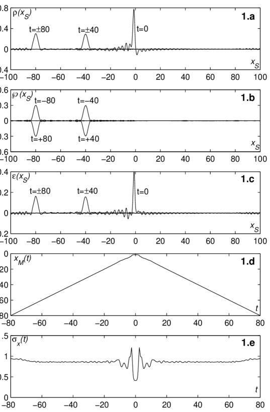
Figure 1: Quantum trajectory for a reflected particle

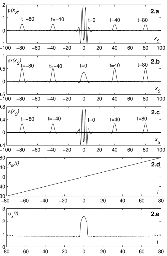
Figure 2: Quantum trajectory for a transmitted particle

Appendix B Brief introduction to the many-particle case

In standard QM, a system of $N$ particles is described by a wave-function $\psi\left(x_{1},\dots,x_{N}\right)$ and the fact that $\psi$ is defined over a configuration space, whose dimension depends on the particles’ number, is a further obstacle to a realistic interpretation of the wave-function; therefore this undesired feature must disappear in the density matrix representation. To be simple, let’s consider a system of two particles moving in one space dimension under the effect of an external potential $V\left(x_{1},x_{2}\right)$; to avoid possible complications which may arise in the case of identical particles, we will further suppose that the two particles have different masses $m_{1}$ and $m_{2}$. The Schrödinger equation for the density matrix $\varphi\left(x_{1},x_{2},y_{1},y_{2}\right)$ is then:

$$i\hbar\frac{\partial\varphi}{\partial t}=-\sum_{i=1}^{2}\frac{\hbar^{2}}{2m_{i}}\left(\frac{\partial^{2}\varphi}{\partial x_{i}^{2}}-\frac{\partial^{2}\varphi}{\partial y_{i}^{2}}\right)+\left[V\!\left(x_{1},x_{2}\right)-V\!\left(y_{1},y_{2}\right)\right]\varphi$$ (88)

In our approach, the solutions of equation (88) are taken to represent individual physical systems instead of statistical mixtures. To eliminate the dependence of $\varphi$ upon the configuration variables $\left(x_{1},y_{1}\right)$ and $\left(x_{2},y_{2}\right)$, we would like to impose the following separability condition:

$$\varphi\left(x_{1},x_{2},y_{1},y_{2},t\right)=\varphi_{1}\left(x_{1},y_{1},t\right)\,\varphi_{2}\left(x_{2},y_{2},t\right)$$ (89)

so that the two functions $\varphi_{1}$ and $\varphi_{2}$ would describe separately the time evolution of the two particles and could be thought to depend upon just one coordinate pair $\left(x,y\right)$, as in the single particle case. Unfortunately, the condition (89) is in general too strong, and may be satisfied only in some special cases, for instance when $V\left(x_{1},x_{2}\right)=V_{1}\left(x_{1}\right)+V_{2}\left(x_{2}\right)$. However, since we know that the observable quantities depend only upon the values of $\varphi$ in the region where $x_{1}\approx y_{1}$ and $x_{2}\approx y_{2}$, we may impose a weaker separability condition: therefore we first define

$$x_{iS}=\frac{1}{2}\left(x_{i}+y_{i}\right)\qquad\qquad\qquad x_{iD}=x_{i}-y_{i}\qquad\qquad i=1,2$$ (90)

and then require that (89) be satisfied only far small values of $x_{1D}$ and $x_{2D}$.

For $x_{1D}=x_{2D}=0$ we then obtain the condition

$$\varphi\Big{|}_{x_{1D}=x_{2D}=0}=\rho_{1}\left(x_{1S},t\right)\,\rho_{2}\left(x_{2S},t\right)$$ (91)

while at first order in $x_{1D}$ and $x_{2D}$ we obtain:

$$-i\hbar\frac{\partial\varphi}{\partial x_{1D}}\Bigg{|}_{x_{1D}=x_{2D}=0} = \mathcal{P}_{1}\left(x_{1S},t\right)\,\rho_{2}\left(x_{2S},t\right)$$ (92)

$$-i\hbar\frac{\partial\varphi}{\partial x_{2D}}\Bigg{|}_{x_{1D}=x_{2D}=0} = \rho_{1}\left(x_{1S},t\right)\,\mathcal{P}_{2}\left(x_{2S},t\right)$$ (93)

If we now extend the definitions (13) and (14) of center of mass and momentum to the two-particle case, we easily obtain

$$Q = Q_{1}+Q_{2}=\int{x_{S}\,\rho_{1}\left(x_{S}\right)\textrm{d}x_{S}}+\int{x_{S}\,\rho_{2}\left(x_{S}\right)\textrm{d}x_{S}}$$ (94)

$$P = P_{1}+P_{2}=\int{\mathcal{P}_{1}\left(x_{S}\right)\textrm{d}x_{S}}+\int{\mathcal{P}_{2}\left(x_{S}\right)\textrm{d}x_{S}}$$ (95)

where we supposed that both $\rho_{1}$ and $\rho_{2}$ satisfy the unitarity condition $\int{\rho_{i}\left(x_{S}\right)\textrm{d}x_{S}}=1$. As for the energy, it is clearly impossible to define two separate energy densities, since the potential energy depends on the position of both particles; this was true already in the classical case.

At first order in $x_{1D}$ and $x_{2D}$, the Schrödinger equation (89) may be decoupled in the two separate equations:

$$\frac{\partial\mathcal{P}_{i}}{\partial x_{S}}=-m\frac{\partial\rho_{i}}{\partial t}\qquad\qquad\qquad i=1,2$$ (96)

which are the natural extensions of the condition (36) to the two-particle case. This decoupling of the Schrödinger equation confirms that solutions satisfying to both (91) and (92)-(93) may indeed exist.

At this point it is clear what should be the definition of quantum trajectories in the two-particle case: we will choose those solutions which satisfy both (91) and (92)-(93) and which remain well localized around their center of mass as $t\to\pm\infty$; this localization condition applies separately to both functions $\rho_{1}$ and $\rho_{2}$. These quantum trajectories represent individual physical systems, while positive superpositions of quantum trajectories represent statistical ensembles; in our approach, all other solutions are devoid of physical meaning. Of course, to be physically acceptable, our quantum trajectories must also satisfy the three fundamental principles, i.e. unitarity, Ehrenfest theorem and energy conservation.

References

- [1] J. Bialynicki-Birula and J. Mycielski, Ann. Phys. , 62 (1976)
- [2] D. Bohm, Phys. Rev. , 166 (1952), ibid. , 180 (1952)
- [3] H. D. Doebner and G. A. Goldin, Phys. Rev. A , 3764 (1996)
- [4] D. Dürr, S. Goldstein and N. Zanghì, Jour. Stat. Phys. , 843 (1992)
- [5] H. Everett, Rev. Mod. Phys. , 454 (1957)
- [6] M. Ferrero, S. F. Huelga and E. Santos, Phys. Rev. A , 5008 (1995)
- [7] G. C. Ghirardi, A. Rimini and T. Weber, Phys. Rev. D , 470 (1986)
- [8] N. Gisin, Phys. Lett. A , 1 (1990)
- [9] K. Hasselmann, Physics Essays, , 311 (1996a)
- [10] Th. Kaluza, Sitzungsber. Preuss. Akad. Wiss. Leipzig (1921), 966
- [11] O. Klein, Z. Phys. (1926) 895
- [12] P. G. Kwiat, P. H. Eberhard, A. M. Steinberg and R. Y. Chiao, Phys. Rev. A , 3209 (1994)
- [13] B. Mielnik, Commun. Math. Phys. , 1 (1969)
- [14] J. Moyal, Proc. Camb. Phil. Soc. , 99 (1949)
- [15] H. Nakazato, Found. Phys. , 1709 (1997)
- [16] L.S.F. Olavo, Quantum Mechanics As A Classical Theory I: Non-relativistic Theory, quant-ph/9503020
- [17] P. Pearle, Phys. Rev. A , 2277 (1989)
- [18] A. Raiteri, A realistic interpretation of the density matrix I: Basic concepts, quant-ph/9812011
- [19] E. Schrödinger, Naturwiss. (1926) 664
- [20] L. E. Szabó, Found. of Phys. Lett. , 421 (1995)
- [21] L. E. Szabó, Int. J. Theor. Phys. , 1751 (1995)
- [22] E. Wigner, Phys. Rev. , 74 (1932)
- [23] W. H. Zurek, Phys. Rev. D , 1516 (1981)
- [24] W. H. Zurek, Phys. Rev. D , 1862 (1982)