A local hidden variable theory for the GHZ experiment

Abstract

A recent analysis by de Barros and Suppes of experimentally realizable GHZ correlations supports the conclusion that these correlations cannot be explained by introducing local hidden variables. We show, nevertheless, that their analysis does not exclude local hidden variable models in which the inefficiency in the experiment is an effect not only of random errors in the detector equipment, but is also the manifestation of a pre-set, hidden property of the particles (“prism models”). Indeed, we present an explicit prism model for the GHZ scenario; that is, a local hidden variable model entirely compatible with recent GHZ experiments.

1 Introduction

De Barros and Suppes [1] give a general analysis of realistic experiments, where experimental error reduces the perfect correlations of the ideal GHZ case. Their analysis makes use of inequalities which are said to be “both necessary and sufficient for the existence of a local hidden variable” for the experimentally realizable GHZ correlations. In applying their analysis to the Innsbruck experiment [2], however, they only count events in which all the detectors fire. While necessary for the analysis of that experiment, they recognize that this selective procedure weakens the argument for the non-existence of local hidden variables. Here we show that they are right and that their analysis does not rule out a whole class of local hidden variable models in which the detection inefficiency is not (only) the effect of the random errors in the detector equipment, but it is a more fundamental phenomenon, the manifestation of a predetermined hidden property of the particles. This conception of local hidden variables was suggested in Fine’s prism model [3] and, arguably, goes back to Einstein (See [5] Chapter 4).

Prism models work well in case of the EPR–Bell experiments. The original model applied to the $2\times 2$ spin-correlation experiments and was in complete accordance with the known experimental results. There appeared, however, a theoretical demand to embed the $2\times 2$ prism models into a large $n\times n$ prism model reproducing all potential $2\times 2$ sub-experiments. This demand was motivated by the idea that the real physical process does not know which directions are chosen in an experiment. On the other hand, it seemed that in the known prism models of the $n\times n$ spin-correlation experiment the efficiencies tended to zero, if $n\rightarrow\infty$, which contradicts what we expect of actual experiments. This contradiction was recently resolved in [10] and [11], which show that there is a wide class of physically plausible $\infty\times\infty$ prism models with high efficiency ($\leq 0.82$).

In the first part of this paper we explain the principle difference between the prism models and the local hidden variable models to which de Barros and Suppes’ analysis applies. In the second part, we present an explicit prism model for the GHZ scenario, a local hidden variable model that is entirely compatible with recent GHZ experiments.

2 The GHZ experiment

Figure 1: A three-particle beam-entanglement interferometer

Greenberger, Horne, Shimony and Zeilinger [7] developed a proof of the Bell theorem without using inequalities. For the GHZ example consider three entangled photons flying apart along three different straight lines in the horizontal plane (Fig. 1). Assume that the (polarization part of the) quantum state of the three-photon system is

$$\Psi=\frac{1}{\sqrt{2}}\left(\left|H\right\rangle_{1}\otimes\left|H\right\rangle_{2}\otimes\left|V\right\rangle_{3}+\left|V\right\rangle_{1}\otimes\left|V\right\rangle_{2}\otimes\left|H\right\rangle_{3}\right)$$ (1)

One can transform the polarization degree of freedom into the momentum degree of freedom by means of polarizing beam splitters (see [12]). So the quantum state of the system can be written also in the following form:

$$\Psi=\frac{1}{\sqrt{2}}\left(\left|a\right\rangle_{1}\otimes\left|b\right\rangle_{2}\otimes\left|c\right\rangle_{3}+\left|a^{\prime}\right\rangle_{1}\otimes\left|b^{\prime}\right\rangle_{2}\otimes\left|c^{\prime}\right\rangle_{3}\right)$$

where $\left|a\right\rangle_{1}$ denotes the particle 1 in beam $a$, etc. A straightforward interferometric calculation ([7], p. 1141) shows that the probabilities of detections are

$$\begin{array}[]{rcl}p^{\Psi}_{A^{+}B^{+}C^{+}}\left(\phi_{1},\phi_{2},\phi_{3}\right)&=&\frac{1}{8}\left(1+\sin\left(\phi_{1}+\phi_{2}+\phi_{3}\right)\right)\\ p^{\Psi}_{A^{-}B^{+}C^{+}}\left(\phi_{1},\phi_{2},\phi_{3}\right)&=&\frac{1}{8}\left(1-\sin\left(\phi_{1}+\phi_{2}+\phi_{3}\right)\right)\\ &\textrm{etc}.&\end{array}$$ (2)

(If the number of minuses on the detector labels is even, there is a plus sign; if odd, there is a minus sign.) Introduce the following result functions

$$A\left(\phi_{1}\right)=\left\{\begin{array}[]{ll}1&{\textrm{if the detector }}A^{+}\textrm{ fires}\\ -1&{\textrm{if the detector }}A^{-}\textrm{ fires}\end{array}\right.$$

$B\left(\phi_{2}\right)$ and $C\left(\phi_{3}\right)$ have the same meaning for particles $2$ and $3$. One can also show that in state $\Psi$ the expectation value of the product of the three outcomes is

$$E\left(A\left(\phi_{1}\right)B\left(\phi_{2}\right)C\left(\phi_{3}\right)\right)=\sin\left(\phi_{1}+\phi_{2}+\phi_{3}\right)$$

Consider the following choices of angles:

$$\begin{array}[]{rcl}\Omega_{1}&=&A\left(\pi/2\right)B\left(0\right)C\left(0\right)\\ \Omega_{2}&=&A\left(0\right)B\left(\pi/2\right)C\left(0\right)\\ \Omega_{3}&=&A\left(0\right)B\left(0\right)C\left(\pi/2\right)\\ \Omega_{4}&=&A\left(\pi/2\right)B\left(\pi/2\right)C\left(\pi/2\right)\end{array}$$ (3)

In this case we obtain perfect correlations:

$$E(\Omega_{1})=E(\Omega_{2})=E(\Omega_{3}) = 1$$ (4)

$$E(\Omega_{4}) = -1$$ (5)

So far this is standard quantum mechanics. One can make a Kochen–Specker/EPR-type argument, however, if one assumes that in $\Psi$ predetermined values, revealed by measurement, are assigned to the six observables

$$A\left(\pi/2\right),A\left(0\right),B\left(\pi/2\right),B\left(0\right),C\left(\pi/2\right),C\left(0\right)$$ (6)

By virtue of (4) and (5) these values have to satisfy the following constraints:

$$\begin{array}[]{rcccl}\Omega_{1}&=&A\left(\pi/2\right)B\left(0\right)C\left(0\right)&=&1\\ \Omega_{2}&=&A\left(0\right)B\left(\pi/2\right)C\left(0\right)&=&1\\ \Omega_{3}&=&A\left(0\right)B\left(0\right)C\left(\pi/2\right)&=&1\\ \Omega_{4}&=&A\left(\pi/2\right)B\left(\pi/2\right)C\left(\pi/2\right)&=&-1\end{array}$$ (7)

Then a contradiction is immediate if we take the product of equations (7). Each value appears twice so, whatever the assigned values are, the left hand side is a positive number, whereas the right side is $-1$.

3 De Barros and Suppes’ inequalities

De Barros and Suppes approach the above contradiction in the following way. Without loss of generality, the space of hidden variable can be identified with ${\mathcal{O}}=\{+,-\}^{6}$, the set of the $2^{6}=64$ different 6-tuples of possible combinations of the values (6). Then the GHZ contradiction amounts to the assertion that no probability measure over $\mathcal{O}$ reproduces the expectation values (4) and (5). De Barros and Suppes demonstrate this by concentrating on the product observables ($\Omega_{1},\dots,\Omega_{4}$) for which they derive a system of inequalities that play the same role for GHZ that the general form of the Bell inequalities do for EPR-Bohm type experiments [4]; namely, they provide necessary and sufficient conditions for a certain class of local hidden variable models. The first of their inequalities is just

$$-2\leq E(\Omega_{1})+E(\Omega_{2})+E(\Omega_{3})-E(\Omega_{4})\leq 2$$

and clearly this is violated by (4) and (5). Moreover if, due to inefficiencies in the detectors or to dark photon detection, the observed correlations were reduced by some factor $\varepsilon$; that is

$$E(\Omega_{1})=E(\Omega_{2})=E(\Omega_{3}) = 1-\varepsilon$$ (8)

$$E(\Omega_{4}) = -1+\varepsilon$$ (9)

then, it follows immediately from this inequality that, “the observed correlations are only compatible with a local hidden variable theory” if $\varepsilon>\frac{1}{2}$. De Barros and Suppes made a detailed analysis of the detection errors and the dark photon detections in the realistic detector equipments, and concluded that these phenomena do not yield such a large $\varepsilon$.

As in the case of the Bell inequalities, however, the de Barros and Suppes derivation starts with the assumption that the variables in (6) are two valued (either $+1$ or $-1$). Since we consider the detection/emission ratio as of more fundamental origin, in the prism models developed in the next sections, the variables can take on a third value,“$D$”, corresponding to an inherent “no show” or defectiveness. In the Bell-EPR case we know that the existence of local hidden variables of this more general type are governed by a different system of inequalities. For the inversion symmetric 2x2 case inequalities providing necessary and sufficient conditions for prism models were derived in [6]. We do not have a comparable system characterizing prism models for GHZ type experiments but we will show that GHZ experiments can be modeled by just such local hidden variable theories. Indeed we will give an explicit prism model for a GHZ experiment (with perfect detectors and with zero dark-photon detection probability). We will also show that our model is completely compatible with the results measured in the Innsbruck experiment.

4 A toy prism model of the GHZ experiment

The prism model of the GHZ experiment is a local, deterministic hidden variable theory, in which the hidden variables predetermine not only the outcomes of the corresponding measurements, but also predetermine whether or not an emitted particle arrives to the detector and becomes detected. Consequently, the space $\Lambda$ of hidden variables ought to be a subset of $\{+,-,D\}^{6}$. Each element of $\Lambda$ is a 6-tuple that corresponds to combinations like

$$\left(A(\pi/2),A(0),B(\pi/2),B(0),C(\pi/2),C(0)\right)=(+-D-++)$$

which, for example, stands for the case when particle 1 is predetermined to produce the outcome $+1$ if $\phi_{1}=\pi/2$, $-1$ if angle $\phi_{1}=0$ in the measurement, particle 2 is $\pi/2$-defective, i.e., it gives no outcome if $\phi_{2}=\pi/2$, but produces an outcome $-1$ if $\phi_{2}=0$, particle 3 produces outcome $+1$ for both cases. The essential feature of this conception of hidden variables is that the “values” $A_{\lambda}(\pi/2),A_{\lambda}(0),B_{\lambda}(\pi/2),\dots$ are “prismed” in the sense that, formally, a new “value” is introduced, “$D$”, corresponding to the case when the particle is predetermined not to produce an outcome.

Each GHZ event will be represented as a subset $U$ of $\Lambda$. For instance

$$U_{\{A(\pi/2)=+\}\&\{B(0)=-\}\&\{C(0)=-\}}$$

stands for the triple detection $A^{+}B^{-}C^{-}$ with angles $(\pi/2,0,0)$.

We have seen that, if determinate values are assigned to all the observables, quantum mechanics yields contradictory correlations (7) among the measurement outcomes at the three stations. Although these four correlations are enough for the stated GHZ contradiction, our hidden variable model must be consistent with quantum mechanics in a wider sense: the probability measure $p$ we are going to define on $\Lambda\subset\{+,-,D\}^{6}$ must satisfy further constraints, following from (2):

$$\begin{array}[]{lcr}p\left(U_{\{A(x)=i\}\&\{B(y)=j\}\&\{C(z)=k\}}|U^{triple}_{(x,y,z)}\right)&\\ =\frac{1}{8}\left[1+ijk\sin(x+y+z)\right]&\\ \ \ \ \ \ \ \ \ \ \ \ \ \ \ \ \ \ \ \ \ \ \ \ \ \ \textrm{for all }\begin{array}[]{rcl}x,y,z&=&\frac{\pi}{2},0\\ i,j,k&=&\pm 1\end{array}&\end{array}$$ (10)

where $U^{triple}_{(x,y,z)}=U_{\{A(x)\neq D\}\&\{B(y)\neq D\}\&\{C(z)\neq D\}}$, the event of triple detection.

Constraints (7) correspond to the fact that some of these probabilities are zero, which rule out a large number of 6-tuples. One can show (and easily verify by computer) that from the $3^{6}=729$ elements of $\{+,-,D\}^{6}$ there remains 409 which satisfy (7). For example:

• $(-++-DD)$ is allowed, because, in this case, whatever the chosen experimental setup, there is no detection at station 3, consequently there is no triple coincidence detection.

• $(D--DD+)$ is allowed because for any measurement setup either the outcome triad satisfies the constraints or there is no triple coincidence at all.

• $(---D+-)$ is not allowed, because if the chosen angles were $\left(\pi/2,\pi/2,\pi/2\right)$ then the results would be $A(\pi/2)=-$, $B(\pi/2)=-$ and $C(\pi/2)=+$, which would contradict the constraint $\Omega_{4}=-1$.

There is a prism model on the hidden variable space consisting of these left 409 elements. However, in order to achieve better detection/emission efficiencies, and also to simplify the model, we will refine $\Lambda$ further. The 409 combinations form four disjoint subsets: 217 of them correspond to the situation where there is no triple detection at all, regardless of the angles chosen at the three stations; 48 combinations produce a triple detection coincidence at only one, and 96 at two triads of angles (these 48 and 96 form a prism model for GHZ all by themselves) and the remaining 48 combinations produce a triple coincidence with four different triads of experimental setups. Clearly we achieve the best efficiency if we take for $\Lambda$ the fourth subset, listed in Table I, and simply omit all the others.

$$\begin{array}[]{rcl}\lambda_{1}$=$(----D+)\\ \lambda_{2}$=$(---D-+)\\ \lambda_{3}$=$(---+-D)\\ \lambda_{4}$=$(--D-++)\\ \lambda_{5}$=$(--D+--)\\ \lambda_{6}$=$(--+-+D)\\ \lambda_{7}$=$(--+D+-)\\ \lambda_{8}$=$(--++D-)\\ \lambda_{9}$=$(-D---+)\\ \lambda_{10}$=$(-D-+--)\\ \lambda_{11}$=$(-D+-++)\\ \lambda_{12}$=$(-D+++-)\\ \lambda_{13}$=$(-+---D)\\ \lambda_{14}$=$(-+-D--)\\ \lambda_{15}$=$(-+-+D-)\\ \lambda_{16}$=$(-+D--+)\\ \lambda_{17}$=$(-+D++-)\\ \lambda_{18}$=$(-++-D+)\\ \lambda_{19}$=$(-++D++)\\ \lambda_{20}$=$(-++++D)\\ \lambda_{21}$=$(D---++)\\ \lambda_{22}$=$(D--+-+)\\ \lambda_{23}$=$(D-+-+-)\\ \lambda_{24}$=$(D-++--)\\ \end{array}\ \ \ \begin{array}[]{rcl}\lambda_{25}$=$(D+----)\\ \lambda_{26}$=$(D+-++-)\\ \lambda_{27}$=$(D++--+)\\ \lambda_{28}$=$(D+++++)\\ \lambda_{29}$=$(+---+D)\\ \lambda_{30}$=$(+--D++)\\ \lambda_{31}$=$(+--+D+)\\ \lambda_{32}$=$(+-D-+-)\\ \lambda_{33}$=$(+-D+-+)\\ \lambda_{34}$=$(+-+-D-)\\ \lambda_{35}$=$(+-+D--)\\ \lambda_{36}$=$(+-++-D)\\ \lambda_{37}$=$(+D--+-)\\ \lambda_{38}$=$(+D-+++)\\ \lambda_{39}$=$(+D+---)\\ \lambda_{40}$=$(+D++-+)\\ \lambda_{41}$=$(++--D-)\\ \lambda_{42}$=$(++-D+-)\\ \lambda_{43}$=$(++-++D)\\ \lambda_{44}$=$(++D---)\\ \lambda_{45}$=$(++D+++)\\ \lambda_{46}$=$(+++--D)\\ \lambda_{47}$=$(+++D-+)\\ \lambda_{48}$=$(++++D+)\end{array}$$

Table 1:

For instance the event “$B(0)=+$” corresponds to

$$U_{\{B(0)=+\}}=\left(\lambda_{3},\lambda_{5},\lambda_{8},\lambda_{10},\lambda_{12},\lambda_{15},\lambda_{17},\lambda_{20},\lambda_{22},\lambda_{24},\right.$$

$$\left.\lambda_{26},\lambda_{28},\lambda_{31},\lambda_{36},\lambda_{38},\lambda_{40},\lambda_{43},\lambda_{45},\lambda_{48}\right)$$

Similarly, the event, for example, that “$A(\pi/2)=+$ and $B(0)=+$” is represented by the following subset:

$$U_{\{A(\pi/2)=+\}\&\{B(0)=+\}}=\left(\lambda_{31},\lambda_{33},\lambda_{36},\lambda_{38},\lambda_{40},\lambda_{43},\lambda_{45},\lambda_{48}\right)$$

while, for instance, $U_{\{A(\pi/2)=+\}\&\{B(0)=+\}\&\{C(0)=-\}}=\emptyset$.

Notice that each subset $U_{\{A(x)\neq D\}\&\{B(y)\neq D\}\&\{C(z)\neq D\}}$ – where $x,y,z=\pi/2$ or $0$ – consists of exactly 24 elements of $\Lambda$. These subsets correspond to the triple measurement events that enter into GHZ.

The probability measure on $\Lambda$ must be defined in such a way that the rest of conditions (10) (right hand side is not zero) be satisfied. One can verify by computer that the uniform distribution on $\Lambda$ is a suitable one (each element has probability $\frac{1}{48}$) and the probability model $\left(\Lambda,p\right)$ thus obtained has maximal triple detection efficiency. Indeed, the triple efficiencies are:

$$p(\mathrm{triple\ coincidence}) = p\left(U_{\{A(x)\neq D\}\&\{B(y)\neq D\}\&\{C(z)\neq D\}}\right)=\frac{24}{48}=0.5$$

The only way to increase the efficiency would be to modify the probability distribution over $\Lambda$. Assuming, however, that for such a non-uniform distribution the triple coincidence efficiency is still independent of the chosen experimental setups, we have

$$p(\mathrm{triple\ coincidence}) = \sum_{i=1}^{48}p({\mathrm{triple\ coincidence}}|\lambda_{i})p(\lambda_{i})$$

$$= \sum_{i=1}^{48}\frac{4}{2^{3}}p(\lambda_{i})=\frac{1}{2}$$

independently of the actual probability distribution $p(\lambda_{i})$.

The key idea of a prism model now is to retrieve the quantum probabilities $q(.)$ as the $\Lambda$ space probabilities conditional on the measurement outcomes being nondefective. Due to conditions (10) this feature of the model is automatically provided. Assume, for example, that the chosen angles are $\left\{\pi/2,0,0\right\}$, then

$$q\left(\{A(\pi/2)=-\}\right)$$

$$= p\left(U_{\{A(\pi/2)=-\}}|U_{\{A(\pi/2)\neq D\}\&\{B(0)\neq D\}\&\{C(0)\neq D\}}\right)$$

$$= \frac{p\left(U_{\{A(\pi/2)=-\}}\cap U_{\{A(\pi/2)\neq D\}\&\{B(0)\neq D\}\&\{C(0)\neq D\}}\right)}{p\left(U_{\{A(\pi/2)\neq D\}\&\{B(0)\neq D\}\&\{C(0)\neq D\}}\right)}$$

$$= \frac{p\left(\left\{\lambda_{1},\lambda_{4},\lambda_{5},\lambda_{8},\lambda_{9},\lambda_{10},\lambda_{11},\lambda_{12},\lambda_{15},\lambda_{16},\lambda_{17},\lambda_{18}\right\}\right)}{\frac{24}{48}}$$

$$= \frac{\frac{12}{48}}{\frac{24}{48}}=\frac{1}{2}$$

Similarly, all the other observed single detection probabilities are $\frac{1}{2}$.

To illustrate that constraints (10) are satisfied, consider, for example,

$$q\left(\{A(\pi/2)=+\}\&\{B(\pi/2)=+\}\&\{C(0)=-\}\right)$$

$$= p\left(U_{\{A(\pi/2)=+\}}\cap U_{\{B(\pi/2)=+\}}\cap U_{\{C(0)=-\}}|U^{triple}_{(\frac{\pi}{2},\frac{\pi}{2},0)}\right)$$

$$= \frac{p\left(U_{\{A(\pi/2)=+\}}\cap U_{\{B(\pi/2)=+\}}\cap U_{\{C(0)=-\}}\cap U^{triple}_{(\frac{\pi}{2},\frac{\pi}{2},0)}\right)}{p\left(U^{triple}_{(\frac{\pi}{2},\frac{\pi}{2},0)}\right)}$$

$$= \frac{p\left(\left\{\lambda_{34},\lambda_{35},\lambda_{39}\right\}\right)}{\frac{24}{48}}=\frac{\frac{3}{48}}{\frac{24}{48}}=\frac{1}{8}$$

$$= \frac{1}{8}\left[1-\sin\left(\frac{\pi}{2}+\frac{\pi}{2}+0\right)\right]$$

Finally, due to the selections involved in building the hidden variable space $\Lambda$ the model correctly reproduces the GHZ correlations (7), whenever a triple detection coincidence occurs: For example the observed expectation value of $\Omega_{1}$ is

$$E(\Omega_{1}) = \sum_{\lambda\in U^{triple}_{(\frac{\pi}{2},0,0)}}\Omega_{1}(\lambda)p(\lambda|U^{triple}_{(\frac{\pi}{2},0,0)})=\sum_{\lambda\in U^{triple}_{(\frac{\pi}{2},0,0)}}\frac{p(\lambda)}{p\left(U^{triple}_{(\frac{\pi}{2},0,0)}\right)}=1$$

and, similarly,

$$E(\Omega_{2})=E(\Omega_{3}) = 1$$

$$E(\Omega_{4}) = -1$$

According to the key idea of a prism model, the above expectation values are calculated on sub-ensembles of the emitted particle triads that produce triple detection coincidences. In this respect the prism model mirrors actual GHZ experiments.

5 A complete infinite prism model for the GHZ experiment

In the derivation of the GHZ contradiction we consider only $2\times 2\times 2$ different experimental setups: At each station one considers two possible phase shift angles: $\phi_{1}=\frac{\pi}{2},0$; $\phi_{2}=\frac{\pi}{2},0$; $\phi_{3}=\frac{\pi}{2},0$. In reality, however, the three angles can be chosen arbitrarily, and, according to quantum mechanics, the resulted triple detection probabilities are given in (2). Although the particular $2\times 2\times 2$ scenario suffice to derive a negative statement, the alleged contradiction between the existence of a local hidden variable theory and the observed triple detection probabilities, it is not sufficient for a positive statement about the existence of such a local hidden variable theory. The reason is that if nature works according to such a local hidden variable model, then the model must reproduce all observed triple detection probabilities for all possible combinations of angles $\phi_{1},\phi_{2},\phi_{3}$, since the underlying physical process does not know about the angles chosen by the laboratory assistants at the three stations. That is why we call a toy model the one we constructed in the previous section, and the existence of a complete infinite prism model covering the whole GHZ scenario is still an open question.

Now we are going to construct a complete infinite prism model for the GHZ experiment, which covers the continuum case, when the three phase shift angles can take arbitrary values. For the sake of later convenience introduce the following new parametrization of the phase shift angles:

$$\begin{array}[]{ccc}\alpha&=&\phi_{1}-\frac{\pi}{6}\\ \beta&=&\phi_{2}-\frac{\pi}{6}\\ \gamma&=&\phi_{3}-\frac{\pi}{6}\end{array}$$

Let us sum up what must be represented in the model:

• A continuum set of events corresponding to the detection events,

  $$A^{+}_{\alpha},A^{-}_{\alpha},B^{+}_{\beta},B^{-}_{\beta},C^{+}_{\gamma},C^{-}_{\gamma}\,\,\,\,\,\alpha,\beta,\gamma\in[0,2\pi]$$

  together with the triple conjunctions

  $$\begin{array}[]{c}A^{+}_{\alpha}\wedge B^{+}_{\beta}\wedge C_{\gamma}^{+}\\ A^{+}_{\alpha}\wedge B^{+}_{\beta}\wedge C_{\gamma}^{-}\\ \vdots\\ A^{-}_{\alpha}\wedge B^{-}_{\beta}\wedge C_{\gamma}^{-}\end{array}\,\,\,\,\alpha,\beta,\gamma\in[0,2\pi]$$

  And the “non-defectiveness” events

  $$\begin{array}[]{rcl}A_{\alpha}&=&A^{+}_{\alpha}\vee A^{-}_{\alpha}\\ B_{\beta}&=&B^{+}_{\beta}\vee B^{-}_{\beta}\\ C_{\gamma}&=&C^{+}_{\gamma}\vee C^{-}_{\gamma}\end{array}\,\,\,\,\alpha,\beta,\gamma\in[0,2\pi]$$ (11)

  together with the algebraic relations following from (11).

• The “quantum” probabilities of the above events,

  $$\frac{p\left(A^{+}_{\alpha}\right)}{p\left(A_{\alpha}\right)}=\frac{p\left(A^{-}_{\alpha}\right)}{p\left(A_{\alpha}\right)}=\frac{p\left(B^{+}_{\beta}\right)}{p\left(B_{\beta}\right)}=\frac{p\left(B^{-}_{\beta}\right)}{p\left(B_{\beta}\right)}$$

  $$=\frac{p\left(C_{\gamma}^{+}\right)}{p\left(C_{\gamma}\right)}=\frac{p\left(C_{\gamma}^{-}\right)}{p\left(C_{\gamma}\right)}=\frac{1}{2}$$ (12)

  $$\frac{p\left(A^{+}_{\alpha}\wedge B^{+}_{\beta}\wedge C_{\gamma}^{+}\right)}{p\left(A_{\alpha}\wedge B_{\beta}\wedge C_{\gamma}\right)}=\frac{p\left(A^{-}_{\alpha}\wedge B^{-}_{\beta}\wedge C_{\gamma}^{+}\right)}{p\left(A_{\alpha}\wedge B_{\beta}\wedge C_{\gamma}\right)}$$

  $$\frac{p\left(A^{-}_{\alpha}\wedge B^{+}_{\beta}\wedge C_{\gamma}^{+}\right)}{p\left(A_{\alpha}\wedge B_{\beta}\wedge C_{\gamma}\right)}=\frac{p\left(A^{+}_{\alpha}\wedge B^{-}_{\beta}\wedge C_{\gamma}^{-}\right)}{p\left(A_{\alpha}\wedge B_{\beta}\wedge C_{\gamma}\right)}$$

  $$=\frac{1}{8}\left(1-\cos\left(\alpha+\beta+\gamma\right)\right)$$ (13)

  $$\frac{p\left(A^{-}_{\alpha}\wedge B^{+}_{\beta}\wedge C_{\gamma}^{+}\right)}{p\left(A_{\alpha}\wedge B_{\beta}\wedge C_{\gamma}\right)}=\frac{p\left(A^{+}_{\alpha}\wedge B^{-}_{\beta}\wedge C_{\gamma}^{+}\right)}{p\left(A_{\alpha}\wedge B_{\beta}\wedge C_{\gamma}\right)}$$

  $$\frac{p\left(A^{+}_{\alpha}\wedge B^{+}_{\beta}\wedge C_{\gamma}^{-}\right)}{p\left(A_{\alpha}\wedge B_{\beta}\wedge C_{\gamma}\right)}=\frac{p\left(A^{-}_{\alpha}\wedge B^{-}_{\beta}\wedge C_{\gamma}^{-}\right)}{p\left(A_{\alpha}\wedge B_{\beta}\wedge C_{\gamma}\right)}$$

  $$=\frac{1}{8}\left(1+\cos\left(\alpha+\beta+\gamma\right)\right)$$ (14)

  in accordance with (2). Probabilities $p\left(A_{\alpha}\right)$, $p\left(B_{\beta}\right)$, $p\left(C_{\gamma}\right)$ and $p\left(A_{\alpha}\wedge B_{\beta}\wedge C_{\gamma}\right)$ are the “single and triple detection efficiencies”.

• The obvious symmetry of the whole experimental setup: None of the three stations is privileged. That is,

  $$p\left(A_{\alpha}\right)=p\left(B_{\beta}\right)=p\left(C_{\gamma}\right)=\omega=\textrm{constant}$$ (15)

  $$p\left(A_{\alpha}\wedge B_{\beta}\wedge C_{\gamma}\right)=p\left(A_{\beta}\wedge B_{\alpha}\wedge C_{\gamma}\right)$$

  $$=p\left(A_{\gamma}\wedge B_{\beta}\wedge C_{\alpha}\right)=\ldots$$ (16)

Figure 2: The hidden variable space is the union of eight regions $G^{+++}$, $G^{++-}$,…$G^{---}$. The first one is shown in the figure

Now, the local hidden variable model we are going to construct is based on the hidden variable space consisting of eight regions $G^{+++}$, $G^{-++}$, $G^{+-+}$ ,… $G^{---}$. Each one is a space $S^{1}\times S^{1}\times S^{1}$ , represented by a cube of size $(2\pi)\times(2\pi)\times(2\pi)$, in which the points of coordinate $0$ and $2\pi$ are identified.(The first such region $G^{+++}$ is shown in Fig. 2.) The normalized probability measure is given by the eight non-negative density functions $\rho^{+++},\ldots\rho^{---}$, such that

$$\int_{0}^{2\pi}\int_{0}^{2\pi}\int_{0}^{2\pi}\rho^{+++}(x,y,z)dxdydz$$

$$+\int_{0}^{2\pi}\int_{0}^{2\pi}\int_{0}^{2\pi}\rho^{-++}(x,y,z)dxdydz$$

$$\ldots+\int_{0}^{2\pi}\int_{0}^{2\pi}\int_{0}^{2\pi}\rho^{---}(x,y,z)dxdydz = 1$$

The events are represented in the following way:

$$A_{\alpha}^{+} = \left\{(x,y,z)\in G^{+++}\left|\alpha\leq x\leq\alpha+\Delta\right.\right\}$$

$$\cup \left\{(x,y,z)\in G^{+-+}\left|\alpha\leq x\leq\alpha+\Delta\right.\right\}$$

$$\cup \left\{(x,y,z)\in G^{+--}\left|\alpha\leq x\leq\alpha+\Delta\right.\right\}$$

$$\cup \left\{(x,y,z)\in G^{+--}\left|\alpha\leq x\leq\alpha+\Delta\right.\right\}$$

$$A_{\alpha}^{-} = \left\{(x,y,z)\in G^{-++}\left|\alpha\leq x\leq\alpha+\Delta\right.\right\}$$

$$\cup \left\{(x,y,z)\in G^{-+-}\left|\alpha\leq x\leq\alpha+\Delta\right.\right\}$$

$$\cup \left\{(x,y,z)\in G^{--+}\left|\alpha\leq x\leq\alpha+\Delta\right.\right\}$$

$$\cup \left\{(x,y,z)\in G^{---}\left|\alpha\leq x\leq\alpha+\Delta\right.\right\}$$

$$\vdots$$

$$C_{\gamma}^{-} = \left\{(x,y,z)\in G^{++-}\left|\gamma\leq z\leq\gamma+\Delta\right.\right\}$$

$$\cup \left\{(x,y,z)\in G^{-+-}\left|\gamma\leq z\leq\gamma+\Delta\right.\right\}$$

$$\cup \left\{(x,y,z)\in G^{+--}\left|\gamma\leq z\leq\gamma+\Delta\right.\right\}$$

$$\cup \left\{(x,y,z)\in G^{---}\left|\gamma\leq z\leq\gamma+\Delta\right.\right\}$$

$$A^{+}_{\alpha}\wedge B^{+}_{\beta}\wedge C^{+}_{\gamma} = \left\{(x,y,z)\in G^{+++}\left|\begin{array}[]{c}\alpha\leq x\leq\alpha+\Delta\\ \beta\leq y\leq\beta+\Delta\\ \gamma\leq z\leq\gamma+\Delta\end{array}\right.\right\}$$

$$A^{-}_{\alpha}\wedge B^{+}_{\beta}\wedge C^{+}_{\gamma} = \left\{(x,y,z)\in G^{-++}\left|\begin{array}[]{c}\alpha\leq x\leq\alpha+\Delta\\ \beta\leq y\leq\beta+\Delta\\ \gamma\leq z\leq\gamma+\Delta\end{array}\right.\right\}$$

$$\vdots$$

$$A_{\alpha} = \left\{(x,y,z)\in G^{+++}\left|\alpha\leq x\leq\alpha+\Delta\right.\right\}$$

$$\cup \left\{(x,y,z)\in G^{-++}\left|\alpha\leq x\leq\alpha+\Delta\right.\right\}$$

$$\vdots$$

$$\cup \left\{(x,y,z)\in G^{---}\left|\alpha\leq x\leq\alpha+\Delta\right.\right\}$$

$$\vdots$$

$$C_{\gamma} = \left\{(x,y,z)\in G^{+++}\left|\gamma\leq z\leq\gamma+\Delta\right.\right\}$$

$$\cup \left\{(x,y,z)\in G^{-++}\left|\gamma\leq z\leq\gamma+\Delta\right.\right\}$$

$$\vdots$$

$$\cup \left\{(x,y,z)\in G^{---}\left|\gamma\leq z\leq\gamma+\Delta\right.\right\}$$

One can easily verify that the required symmetries (15) and (III.) are satisfied by the following Ansatz:

$$\rho^{+++}(x,y,z)=\rho^{--+}(x,y,z)=\rho^{-+-}(x,y,z)$$

$$=\rho^{+--}(x,y,z)=f(x+y+z)\rho(x+y+z)$$ (19)

$$\rho^{-++}(x,y,z)=\rho^{+-+}(x,y,z)=\rho^{++-}(x,y,z)$$

$$=\rho^{---}(x,y,z)=\left(\frac{1}{4}-f(x+y+z)\right)\rho(x+y+z)$$ (20)

where $\rho$ and $f$ are arbitrary non-negative functions satisfying the following conditions:

$$\int_{0}^{2\pi+\Delta}\int_{0}^{2\pi+\Delta}\int_{0}^{2\pi+\Delta}\rho(x+y+z)dxdydz=1$$ (21)

$$0\leq f(w)\leq\frac{1}{4}\,\,\,\,\,\,\,w\in[0,6\pi]$$ (22)

Now, the probability measure on the hidden variable space, that is, the functions $\rho$ and $f$ must be defined in such a way that the quantum probabilities (II.)-(II.) are reproduced. Due to (19)-(22), equation (II.) is automatically satisfied, and if $\rho$ and $f$ satisfy (II.) then they automatically satisfy (II.). So, there remains only one equation to be solved:

$$\frac{\int_{\gamma}^{\gamma+\Delta}\int_{\beta}^{\beta+\Delta}\int_{\alpha}^{\alpha+\Delta}f(x+y+z)\rho(x+y+z)dxdydz}{\int_{\gamma}^{\gamma+\Delta}\int_{\beta}^{\beta+\Delta}\int_{\alpha}^{\alpha+\Delta}\rho(x+y+z)dxdydz}$$

$$=\frac{1}{8}\left(1-\cos\left(\alpha+\beta+\gamma\right)\right)$$ (23)

So we are looking for non-negative real functions $\rho(w)$ and $f(w)$ defined on the interval $\left[0,6\pi\right]$, satisfying (5) and the conditions (21) and (22). We know that $f(w)=0$ if $w\in\bigcup_{k=0,1,2,3}\left[2k\pi,2k\pi+3\Delta\right]$ because $\cos\left(2k\pi\right)=1,\,\,k=0,1,2,3$, and $f(z)=\frac{1}{4}$ if $w\in\bigcup_{k=0,1,2}\left[(2k+1)\pi,(2k+1)\pi+3\Delta\right]$ because $\cos\left((2k+1)\pi\right)=-1,\,\,k=0,1,2$. These two regions must be disjoint, consequently $\Delta\leq\frac{\pi}{3}$, which means – in this model – a limitation for the single detection efficiency: $\omega\leq\frac{1}{6}$. Let us chose $\Delta=0.9\frac{\pi}{3}$, $\omega=15\%$.

Figure 3: A numerical solution of the integral equation (5) for function $f$

Figure 4: A numerical solution of the integral equation (5) for function $\rho$

Figure 5: This is two curves in coincidence: One is the numeric result of the left hand side of equation (5), the other is the function on the right hand side

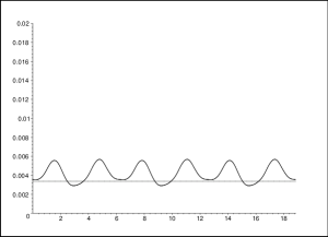
Figure 6: The dependence of the triple detection efficiency on $\alpha+\beta+\gamma$. The horizontal line represents the value $\omega^{3}=0.34\%$ corresponding to the case of independence

One can solve (5) numerically. Figure 3 and 4 show the numerical solutions for functions $f$ and $\rho$. Figure 5 illustrates the high precision of the numerical solution. The triple detection efficiency depends on the phase shift angles. Figure 6 shows the dependence of the triple detection efficiency on $\alpha+\beta+\gamma$. The minimal triple efficiency – in this example – is about 0.2%.

6 Recent experiments

Figure 7 shows the schematic drawing of the experimental setup of the Innsbruck experiment [2]. With a small probability, an UV pulse causes a double pair creation in the non-linear crystal (BBO). The two pairs created within the window of observation are indistinguishable. It can be shown that by restricting the ensemble to the sub-ensemble of cases when all of the four detectors, $T,D_{1},D_{2},D_{3}$ fire, we obtain the following quantum state:

$$\underbrace{\frac{1}{\sqrt{2}}\left(\left|H\right\rangle_{1}\otimes\left|H\right\rangle_{2}\otimes\left|V\right\rangle_{3}+\left|V\right\rangle_{1}\otimes\left|V\right\rangle_{2}\otimes\left|H\right\rangle_{3}\right)}_{\Psi_{GHZ}}\otimes\left|H\right\rangle_{T}$$

where $\left|H\right\rangle_{T}$ denotes the state of the photon at detector $T$. This quantum state corresponds to a four-particle system consisting of an entangled three-photon system in GHZ state, and a fourth independent photon. So we may assume that the statistics observed on the sub-ensemble conditioned by the four-fold coincidences are the same as those taken on the sub-ensemble conditioned by the triple detections at $D_{1},D_{2}$ and $D_{3}$. What is important from our point of view is that any further experimental observations testing the GHZ correlations, which are based on the above described preparation of GHZ entangled states, will be performed on selected sub-ensembles conditioned by the triple coincidence detections. Therefore, all of these experimental observations will be treated by our local hidden variable model.

Figure 7: The experimental setup for demonstration of GHZ entanglement for spatially separated photons

Finally, notice that triple detections, where permitted by the prism model, are subject to ordinary sorts of external detection error. If the external detection efficiency is, say, $d$, then triple outcomes having probability

$$p(\mathrm{triple\ detection}|\mathrm{none\ are\ defective})=1$$

according to the ideal case specified in the model, will have a reduced probability of $d^{3}$, as in the usual analysis of random errors. Similarly we can take into account the non-zero probability of random dark photon detections and make a calculation like that of de Barros and Suppes, resulting in the modified expectation values (8) and (9). Thus our local hidden variable framework allows for the usual techniques of error analysis to treat experimental inefficiencies reflected in the actual observations.

The research was partly supported by the OTKA Foundation, No. T025841 and No. T032771 (L. E. Szabó).

References

• [1] J. A. De Barros and P. Suppes, Phys. Rev. Lett. 84, 793 (2000).
• [2] D. Bouwmeester, J. Pan, M. Daniell, H. Weinfurter and A. Zeilinger, Phys. Rev. Lett. 82, 1345 (1999).
• [3] A. Fine, Synthese 50, 279 (1982).
• [4] A. Fine, Phys. Rev. Lett. 48, 291 (1982).
• [5] A, Fine, The Shaky Game: Einstein, Realism and the Quantum Theory, 2nd edition, (University of Chicago Press, Chicago, 1996).
• [6] A. Garg and D. Mermin, Phys. Rev. D 35, 3831 (1987).
• [7] D. M. Greenberger, M. A. Horne, A. Shimony and A. Zeilinger, Am. J. Phys. 58, 1131 (1990).
• [8] J.-A. Larsson, Phys. Rev. A57, R3145 (1998).
• [9] J.-A. Larsson, Phys. Rev. A59, 4801 (1999).
• [10] J.-A. Larsson, Phys. Lett. A256, 245 (1999).
• [11] L. E. Szabó, Foundations of Physics 30, 1891 (2000).
• [12] A. Zeilinger, M. A. Horne, H. Weinfurter and M. $\dot{Z}$ukowski, Phys. Rev. Lett. 78, 3031 (1997).