Coherent transport of matter waves

Abstract

A transport theory for atomic matter waves in low-dimensional waveguides is outlined. The thermal fluctuation spectrum of magnetic near fields leaking out of metallic microstructures is estimated. The corresponding scattering rate for paramagnetic atoms turns out to be quite large in micrometer-sized waveguides (approx. 100/s). Analytical estimates for the heating and decoherence of a cold atom cloud are given. We finally discuss numerical and analytical results for the scattering from static potential imperfections and the ensuing spatial diffusion process.
PACS: 03.75.-b Matter waves – 32.80.Lg Mechanical effects of light on atoms and ions – 05.60.C Classical transport – 05.40.-a Fluctuation phenomena and noise

Introduction

Atom optics, the coherent manipulation of atomic matter waves, is currently heading towards miniaturization and integration. Atom guides in both one and two dimensions have been demonstrated Schmiedmayer95 ; Ohtsu96b ; Mlynek98b ; Schmiedmayer98b ; Hinds00 . Recent experiments have studied atoms trapped in electromagnetic solid-state hybrid surface guides (or “atom chips”) Anderson99 ; Schmiedmayer00a ; Prentiss00 ; Schmiedmayer00b . The near future may be expected to see the trapping and manipulation of Bose-condensed atoms in such microtraps Grimm00a . Decoherence is an intriguing issue in this context because of the close proximity of the cold atom cloud to the macroscopic substrate, typically being held at room temperature. Thermal electromagnetic fields thus perturb the atoms, leading to heating, trap loss and scattering Henkel99b ; Henkel99c . The thermal noise spectra are much larger than the blackbody spectrum because the characteristic distances are much smaller than the photon wavelengths for the relevant transition frequencies: the atoms are subject to thermal near fields Henkel00b . It is therefore of much interest to estimate the length and time scales over which the transport of matter waves in atom chips remains coherent.

In this paper, we outline a transport theory for matter waves in low-dimensional waveguides close to metallic microstructures. Such structures are used in current experiments to generate magnetic fields or to reflect optical fields. We focus on paramagnetic atoms and their perturbation by the thermally excited magnetic near field. Scattering rates and noise spectra are computed for a few generic geometries: a metallic half-space, a layer, and a cylindrical wire. A self-consistent transport theory for the atomic Wigner distribution is formulated for a dilute, non-condensed cloud. In the case of a white noise spectrum (that turns out to be an excellent approximation for the magnetic near field), the transport equation is solved analytically, and the atomic decoherence rate is determined. We finally present analytical and numerical calculations for a waveguide with static roughness (due to imperfections in the guiding field, for example).

1 Model

1.1 Perturbation of a trapped spin

We start from an atom trapped in a wave guide potential that restricts its motion to one or two dimensions. We suppose that the transverse degrees of freedom are ‘frozen out’, the atom being in the transverse ground state. In the remaining directions, we assume a free motion. Examples of such waveguides are linear magnetic quadrupole guides formed by currents in one or several parallel wires Schmiedmayer95 ; Anderson99 ; Schmiedmayer00a ; Prentiss00 ; Schmiedmayer00b or planar guides mounted above a surface ‘coated’ with repulsive optical Mlynek98b or magnetic Hinds00 fields. Trapped paramagnetic atoms couple to thermal fluctuations of the magnetic field and will scatter from these at a rate given by Fermi’s Golden Rule

$$\gamma_{\rm i\to f}=\frac{1}{\hbar^{2}}\sum_{i,j=1}^{3}\langle{\rm i}|\mu_{i}|{\rm f}\rangle\langle{\rm f}|\mu_{j}|{\rm i}\rangle B_{ij}(\omega_{\rm if}),$$ (1)

where $B_{ij}(\omega_{\rm if})$ is the magnetic cross correlation tensor (spectral density) and $\hbar\omega_{\rm if}$ is the energy difference between the initial and final states $|{\rm i}\rangle,\,|{\rm f}\rangle$. The correlation tensor $B_{ij}(\omega)$ is calculated in subsection 1.2, where we shall see that it depends on the distance to the metallic microstructures. Its frequency dependence is quite weak, however, because the relevant transition frequencies are at most in the GHz range. Magnetic noise at these frequencies drives spin-flip transitions that, in a magnetostatic trap, put the atom onto a non-trapping potential surface. The concomitant loss rate has been discussed previously Henkel99c . We focus here on the scattering between quasi-plane waves in the same spin state that remain trapped in the waveguide. These transitions correspond to much lower frequencies of the order of the temperature of the atomic cloud (typically in the kHz range). The corresponding photon wavelengths are much larger than the characteristic size of the waveguide structures. For this reason, we may adopt the magnetostatic approximation in order to compute the thermal magnetic field spectral density.

1.2 Magnetic near field

1.2.1 The method.

Fluctuation electrodynamics (or source theory) is a convenient tool to compute the spectral correlation tensor of the electromagnetic field in an inhomogeneous, dissipative environment. Basically, one introduces a fluctuating current density whose spectral density is determined from the imaginary part of the dielectric function. The field radiated by these currents is computed from the Green tensor for the chosen geometry Lifshitz56 ; Varpula84 . It has been shown that this scheme also provides a consistent way to quantize the electromagnetic field in dispersive and absorbing dielectrics Welsch96 ; Knoell98a ; Knoell98b ; Savasta00 (see Barnett97 for further reference).

1.2.2 Low-frequency noise.

For our present purposes, a simplified Green tensor is sufficient: we focus on nonmagnetic media and low frequencies where the magnetostatic approximation is valid. As outlined in appendix A, we find the following expression for the scattering rate (1)

$$\gamma=C_{0}Y_{nn},$$ (2)

where the prefactor is

$$C_{0}=\frac{\left|\langle s|\mu_{n}|s\rangle\right|^{2}}{\hbar^{2}}\frac{k_{\rm B}T}{4\pi^{2}\varepsilon_{0}^{2}c^{4}\varrho}.$$ (3)

Here, $\mu_{n}$ is the projection of the magnetic moment along a static bias field, $|s\rangle$ is the trapped spin state, and $T$, $\varrho$ are temperature and specific resistance of the metallic microstructures. Finally, $Y_{nn}$ is the matrix element along the bias field of a geometric tensor $Y_{ij}$ defined in (37). The scattering rate (2) is of the order of

$$\gamma\sim 75\,{\rm s}^{-1}\frac{(\mu/\mu_{\rm B})^{2}(T/300\,{\rm K})}{(\varrho/\varrho_{\rm Cu})}(Y_{ij}\times 1\,\mu{\rm m}).$$ (4)

(We have taken the specific resistance of copper $\varrho_{\rm Cu}=1.7\times 10^{-6}\,{\rm\Omega\,cm}$ Kittel .) The geometric tensor $Y_{ij}$ (37) has dimension (1/length), and its magnitude is the inverse of the characteristic scale of the waveguide. As a consequence, the scattering rate (4) is quite large for a typical micrometer-size waveguide.

1.2.3 Typical geometries.

We now give the results of the evaluation of the geometric tensor (37) for three generic geometries. For a metallic half-space, we find that

$$Y_{ij}=\frac{\pi t_{ij}}{4z},$$ (5)

where the diagonal tensor $t_{ij}$ has elements $(\frac{3}{2},\frac{3}{2},1)$. Note the long range $1/z$ dependence on distance $z$ Henkel99b .

For a metallic layer of thickness $d$ above a nonconducting substrate, we find

$$Y_{ij}=\frac{\pi t_{ij}d}{4z(z+d)}.$$ (6)

This expression reproduces the result (5) for the metallic half space when the distance $z$ from the upper interface is much smaller than the layer thickness $d$. On the other hand, at large distances a faster decrease $d/z^{2}$ takes over.

Finally, for a cylindrical wire of radius $a$, we found a cumbersome expression involving an elliptic integral. Nevertheless, simple results are obtained for the trace of the geometry tensor in the following limits: (1) If the distance $R$ from the wire axis is large compared to wire radius,

$${\rm tr}\,Y_{ij}\approx\frac{\pi^{2}a^{2}}{2R^{3}}\left[1+\frac{9}{4}\left(\frac{a}{R}\right)^{2}+{}\right.$$

$$\qquad\left.{}+\frac{225}{186}\left(\frac{a}{R}\right)^{4}+{\cal O}[(a/R)^{6}]\right].$$ (7)

Note the even stronger power law decrease $a^{2}/R^{3}$ to leading order compared to the planar geometries. The three-term expansion (7) is reasonably accurate down to $R\geq 1.6\,a$. (2) In the short-distance limit $R-a\ll a$, we recover the flat half-space result (5)

$${\rm tr}\,Y_{ij}\approx\frac{\pi}{R-a}.$$ (8)

In Figure 1, we plot the corresponding scattering rates as a function of distance (i.e., $z$ for the planar guides, $R-a$ for the wire guide). The static bias field at the waveguide center is taken perpendicular to the metallic surface. The scattering rate for the wire is actually overestimated because the trace of the magnetic correlation tensor is used.

1.3 Transport equation

The evolution of a trapped matter wave in the waveguide is conveniently described in terms of a transport equation. This equation allows to characterize the evolution of the single-particle spatial density matrix (or coherence function)

$$\rho({\bf x};{\bf s})=\langle\psi^{*}({\bf x}+{\textstyle\frac{1}{2}}{\bf s})\,\psi({\bf x}-{\textstyle\frac{1}{2}}{\bf s})\rangle,$$ (9)

where the average $\langle\ldots\rangle$ is taken over the spatial and temporal fluctuations of a perturbing potential. Instead of working with the coherence function (9), we formulate the transport equation for the Wigner transform of the density matrix

$$W({\bf x},{\bf p})=\int\!\frac{d^{D}s}{(2\pi\hbar)^{D}}e^{i{\bf p}\cdot{\bf s}/\hbar}\rho({\bf x};{\bf s}),$$ (10)

that may be interpreted as a quasi-probability distribution in phase space. Here and in the following, the coordinates ${\bf x}$ and ${\bf p}$ describe the motion in the $D=1,\,2$ dimensional waveguide.

The quasi-free wave function for the trapped spin state $|s\rangle$ in the waveguide is perturbed by the magnetic potential

$$V({\bf x},t)=\langle s|\mu_{n}|s\rangle B_{n}({\bf x},t),$$ (11)

where $B_{n}$ is again the field component along the static bias field. We now have to take into account both energy and momentum changes in the scattering process. This may be done in terms of a master (or transport equation) for the Wigner distribution. It is derived using second order perturbation theory with respect to $V$, assuming that $V$ has gaussian statistics and doing a multiple-scale expansion of the Bethe-Salpeter equation for the coherence function Keller96 . We find:

$$\Bigl{(}\partial_{t}+\frac{1}{m}{\bf p}\cdot\nabla_{\bf x}+{\bf F}_{\rm ext}\cdot\nabla_{\bf p}\Bigr{)}W({\bf x},{\bf p})=$$ (12)

$$\int\!{\rm d}^{D}p^{\prime}\,S_{V}({\bf p}-{\bf p}^{\prime};E_{p}-E_{p^{\prime}})\left[W({\bf x},{\bf p}^{\prime})-W({\bf x},{\bf p})\right],$$

with the de Broglie dispersion relation $E_{p}=p^{2}/2m$ and where $S({\bf q};\Delta E)$ is the spectral density of the perturbation

$$S_{V}({\bf q};\Delta E)=\frac{1}{\hbar^{2}}\int\!\frac{d^{D}s\,d\tau}{(2\pi\hbar)^{D}}\langle V({\bf x}+{\bf s},t+\tau)\,V({\bf x},t)\rangle\times{}$$

$$\qquad{}\times\,e^{-i({\bf q}\cdot{\bf s}-\Delta E\tau)/\hbar}.$$ (13)

The average $\langle\ldots\rangle$ is again taken with respect to the magnetic noise field. We assume for simplicity that the noise is statistically stationary in time and along the waveguide directions. This is actually the case for linear or planar waveguides parallel to planar structures and for a linear guide parallel to a wire.

The left hand side of the transport equation (12) describes the ballistic motion of the atom subject to the external (deterministic) force ${\bf F}_{\rm ext}$. The right hand side describes the scattering off the magnetic field fluctuations. As a function of the momentum transfer $\bf q$, e.g., the spectral density $S_{V}({\bf q};\Delta E)$ is proportional to the spatial Fourier transform of the potential, as to be expected from the Born approximation for the scattering process ${\bf p}^{\prime}\to{\bf p}={\bf p}^{\prime}+{\bf q}$. The transport equation thus combines in a self-consistent way ballistic motion and scattering processes.

The frequency dependence of the magnetic field noise has already been treated in the previous subsection. We saw that the spectral density is flat in the magnetostatic approximation. The magnetic perturbation can therefore be treated as a white noise. To get the wave vector dependence, we have to evaluate the spatial Fourier transform of the two-point correlation function $B_{ij}({\bf x}_{1},{\bf x}_{2})$. In the magnetostatic limit, it turns out that above a planar metallic layer, the correlation function is similar to a lorentzian, with a correlation length $l_{c}$ parallel to the layer given by the distance $z$ perpendicular to the layer (see figure 2). More details are discussed elsewhere Henkel00b . As a consequence of the finite correlation length, the scattering kernel $S({\bf q};\Delta E)$ in the transport equation (12) exhibits a cutoff for momentum transfers $|{\bf q}|\geq\hbar/l_{c}\approx\hbar/z$. The spatial smoothness of the magnetic field thus limits the possible scattering processes, although arbitrary energy transfers are available from the white noise perturbation.

In the following, we assume a constant force ${\bf F}_{\rm ext}$ and focus on two limiting cases of the transport equation (12): (1) ‘Inelastic transport’ under the influence of white noise perturbations. This is the appropriate limit to estimate the detrimental effects of thermal magnetic fields. (2) ‘Elastic transport’ where a time-independent perturbation is assumed. This allows to describe in the same framework the influence of static roughness in the waveguide potentials from which the atoms scatter. In optical potentials, roughness of this type occurs when the optical fields are scattered from small-scale inhomogeneities in the microstructure Henkel97a . In planar gravito-optical traps based on a planar evanescent wave mirror, the rough optical potential couples efficiently the atomic motion normal and parallel to the mirror Grimm97b . The transport equation is valid as long as one is interested in the evolution on length scales large compared to the correlation length of the roughness. In rough evanescent fields, we find again that this length is typically of order $z$ Henkel97a because high spatial frequencies $K\gg 2\pi/\lambda$ give rise to exponentially damped fields $\propto\exp(-Kz)$.

2 Results

2.1 Inelastic transport

2.1.1 Analytic solution of the transport equation.

For a broad band spectrum of the perturbation, we may neglect the dependence of $S_{V}({\bf q},\Delta E)$ on $\Delta E$. The transport equation (12) then simplifies because the integration over the initial momentum ${\bf p}^{\prime}$ is not restricted by energy conservation. Taking the Fourier transform of the Wigner function $W({\bf x},{\bf p})$ with respect to both variables ${\bf x}$ and ${\bf p}$ (with conjugate variables ${\bf k}$ and ${\bf s}$), it is simple to derive the following solution

$$\tilde{W}({\bf k},{\bf s};t)=\tilde{W}_{0}({\bf k},{\bf s}-\hbar{\bf k}t/m)\,{\rm e}^{-{\rm i}{\bf F}_{\rm ext}\cdot{\bf s}t/\hbar}\times{}$$

$${}\times\exp{\left[-\gamma\int_{0}^{t}\!\!\left(1-C({\bf s}-\hbar{\bf k}t^{\prime}/m)\right)\!{\rm d}t^{\prime}\right]}.$$ (14)

Here, $\tilde{W}_{0}({\bf k},{\bf s})$ is the double Fourier transform of the Wigner function at initial time $t=0$, and $\gamma$ and the normalized spatial correlation function $C({\bf s})$ are related to the correlation function of the perturbation by

$$\gamma C({\bf s})=\frac{1}{\hbar^{2}}\int_{-\infty}^{+\infty}\!d\tau\,\langle V({\bf s},\tau)\,V({\bf 0},0)\rangle,\quad C({\bf 0})=1.$$ (15)

We also note that $\gamma$ is the transition rate $\gamma_{\rm i\to f}$ for scattering processes with zero energy transfer ($\omega_{\rm if}=0$). For a wave guide above a metallic surface, the estimate (4) is hence applicable for the rate $\gamma$.

From the analytic solution (14), it is easily checked that in the absence of the perturbation, the spatial width $\langle\delta x^{2}(t)\rangle$ of a cloud increases ballistically according to $\langle\delta x^{2}(t)\rangle=\langle\delta p^{2}(0)\rangle\,t^{2}/m^{2}$ where $\langle\delta p^{2}(0)\rangle$ is the initial width of the cloud in momentum space (this latter width remains constant in this case, of course).

2.1.2 Spatial decoherence.

More interesting information may be obtained for a nonzero scattering rate $\gamma$. Note that the spatially averaged atomic coherence function is given by

$${\Gamma}({\bf s})=\int\!{\rm d}^{D}{x}\,\rho({\bf x};{\bf s})=\tilde{W}({\bf k}={\bf 0},{\bf s}).$$ (16)

The solution (14) therefore implies that the spatial coherence decays exponentially with time:

$${\Gamma}({\bf s};t)={\Gamma}_{0}({\bf s})\exp{\Bigl{[}-\gamma t(1-C({\bf s}))-{\rm i}{\bf F}\cdot{\bf s}\,t/\hbar\Bigr{]}}.$$ (17)

The decoherence rate depends on the spatial separation between the points where the atomic wave function is probed, and is given by $\gamma({\bf s})=\gamma(1-C({\bf s}))$. It hence saturates to the value $\gamma$ at large separations and decreases to zero for ${\bf s}\to{\bf 0}$. The decay of the coherence function (17) is illustrated in figure 3. One observes that at time scales $t\geq 1/\gamma$, the spatial coherence is reduced to a coherence length $\xi_{\rm coh}\sim l_{c}$. After a few collisions with the fluctuating magnetic field, the long-scale coherence of the atomic wave function is thus lost and persists only over scales smaller than the field’s correlation length (where different points of the wave function ‘see’ essentially the same fluctuations). For larger times $t\gg 1/\gamma$, decoherence proceeds at a smaller rate that is related to momentum diffusion, as we shall see now.

2.1.3 Momentum diffusion at long times.

The behaviour of the atomic momentum distribution at long times may be extracted from an expansion of the analytic solution (17) for small values of ${\bf s}$. Assuming a quadratic dependence of the field’s correlation function, $C({\bf s})\approx 1-s^{2}/l_{c}^{2}$, as one would expect for Lorentzian correlations, we find that the atomic momentum distribution is gaussian at long times; it is centered at ${\bf p}_{0}+{\bf F}_{\rm ext}t$ due to the external force, and its width increases according to a diffusion process in momentum space

$$\langle\delta p^{2}(t)\rangle\approx\langle\delta p^{2}(0)\rangle+\frac{\hbar^{2}\gamma t}{l_{c}^{2}}.$$ (18)

This was to be expected: the atoms perform a random walk in momentum space, exchanging a momentum of order $\hbar/l_{c}$ per scattering time $1/\gamma$. The momentum diffusion coefficient $D_{p}=\hbar^{2}\gamma/l_{c}^{2}$ that may be read off from (18) is consistent with this intuitive interpretation. Physically speaking, the atomic cloud is ‘heated up’ due to the scattering from the fluctuating potential. We note that the rate of change of the atomic kinetic energy in the wave guide plane is the same as the one for the tightly bound motion perpendicular to the metallic surface (see Henkel99c for a calculation of this rate).

Translating the width of the momentum distribution into a spatial coherence length, we find a power-law decay at long times, $\xi_{\rm coh}=l_{c}/\sqrt{\gamma t}$. Finally, a similar calculation yields the width of the atomic cloud in position space: it increases ‘super-ballistically’ at long times, $\langle\delta x^{2}(t)\rangle\propto t^{3}$, as a consequence of heating.

2.2 Elastic transport

A waveguide potential with static roughness leads to energy-conserving scattering. The integration over the initial momenta ${\bf p}^{\prime}$ in the transport equation (12) is then restricted which complicates the analytic solution. We discuss in the following numerical results and an analytic solution for vanishing external force.

2.2.1 Numerical results.

The transport equation may be solved using a split-step propagation method. We alternate between ballistic motion and the scattering. In one dimension, e.g., the transport equation reads

$$\left(\partial_{t}+\frac{p}{m}\partial_{x}+F_{\rm ext}\partial_{p}\right)W(x,p,t)=$$ (19)

$$\gamma(p)\left(W(x,-p,t)-W(x,p,t)\right),$$

where the scattering rate $\gamma(p)$ depends on momentum via the wavevector transfer $|2p/\hbar|$. The solution for pure ballistic transport is described by

$$W(x,p,t+\Delta t)=$$ (20)

$$W(x-(p/m)\Delta t+(F_{\rm ext}/2m)\Delta t^{2},p-F_{\rm ext}\Delta t,t),$$

while the scattering kernel gives

$$\left(\begin{array}[]{c}W(x,p,t+\Delta t)\\ W(x,-p,t+\Delta t)\end{array}\right)=$$ (23)

$$e^{-\gamma(p)\Delta t}\left(\begin{array}[]{cc}\displaystyle{\cosh{\gamma\Delta t}}&\displaystyle{\sinh{\gamma\Delta t}}\\ \displaystyle{\sinh{\gamma\Delta t}}&\displaystyle{\cosh{\gamma\Delta t\par}}\end{array}\right)\left(\begin{array}[]{c}W(x,p,t)\\ W(x,-p,t)\end{array}\right).$$ (28)

For sufficiently small time steps $\Delta t$, the combination of these two steps gives an efficient way to compute the time evaluation of the Wigner distribution.

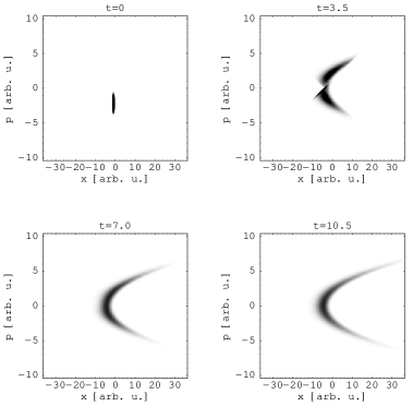
Figure 5: Snapshots of four stages of the temporal evolution of a Wigner distribution accelerated by an external force. The underlying dataset is the same as the one used for figure 4.

We present results for the two cases of an atomic sample moving in a wave guide with a static rough potential with and without an external force applied that accelerates the sample. In the first case we observe that for short times the average motion is ballistic, which is shown in figure 4: the cloud is accelerated according to $\langle x(t)\rangle=\langle x(0)\rangle+\langle p(0)/m\rangle t+(F_{\rm ext}/2m)t^{2}$. However, at longer times a different behaviour takes over and the average position shows a linear drift. We also observe a monotonic increase with time of the spatial width $\langle\delta x^{2}(t)\rangle$ of the atomic cloud. Figure 4 shows that this increase is approximately linear, as would be the case for a spatial diffusion process. The transient ballistic regime may be understood qualitatively by inspection of the average momentum $\langle p(t)\rangle$ and momentum width $\langle\delta p^{2}(t)\rangle$, also shown in figure 4, as well as of the snapshots of the temporal evolution in phase space (figure 5): the elastic scattering transfers atoms from negative velocities to positive velocities until the average velocity vanishes. This is accompanied by an increase of the momentum spread. At the end of the transient regime, both the momentum spread increase slows down and the motion in position space is no longer ballistic. Note that the deceleration by the scattering potential is faster than expected from the short time acceleration $\langle p(t)\rangle=\langle p(0)\rangle+F_{\rm ext}t$.

For the case of a vanishing external force we now show that the characteristic behaviour of the atomic cloud can also be obtained analytically. The discussion is restricted to $D=1$ for simplicity.

2.2.2 Analytical estimate of the diffusion coefficient.

In the absence of an external force, the momentum $p$ enters the transport equation only as a parameter, and we are left with a coupled system for the Wigner functions $W(x,\pm p,t)$ [cf. also (23)]. Using a spatial Fourier transform and a temporal Laplace transform (with conjugate variables $k$ and $\zeta$), it is straightforward to obtain the following solution

$$\tilde{W}(k,\pm p;\zeta)=$$ (29)

$$\frac{(\gamma(p)+\zeta-{\rm i}kp/m)\tilde{W}_{0}(k,+p)+\gamma(p)\tilde{W}_{0}(k,-p)}{\zeta^{2}+2\gamma(p)\zeta+k^{2}p^{2}/m^{2}},$$

where $\tilde{W}_{0}(k,+p)$ is the initial (Fourier transformed) Wigner function. The smallest of the denominator’s roots $\zeta_{1,\,2}$ determines the long-time behaviour of the Wigner function. For small values of $k$ (corresponding to large spatial scales), it is given by

$$\zeta_{\rm min}\approx-\frac{k^{2}p^{2}}{2m^{2}\gamma(p)}.$$ (30)

For a Wigner function with gaussian initial data, we thus find the following long-time asymptotics:

$$t\to\infty:$$

$$\langle x(t)\rangle=\langle x(0)\rangle+\frac{p}{2m\gamma(p)},$$ (31)

$$\langle\delta x^{2}(t)\rangle=\langle\delta x^{2}(0)\rangle+\frac{p^{2}t}{2m^{2}\gamma(p)}.$$ (32)

The average position thus tends to a constant, that is displaced by the free flight distance during the scattering time $1/\gamma(p)$. For longer times, the ‘forward’ and ‘backward’ moving Wigner distributions $W(x,\pm p,t)$ have the same weight, and there is no spatial displacement on average. The spatial width increases linearly with time, in accordance with a random walk: for each scattering time $1/\gamma(p)$, a position step $\sim p/m\gamma(p)$ is performed in a random direction.

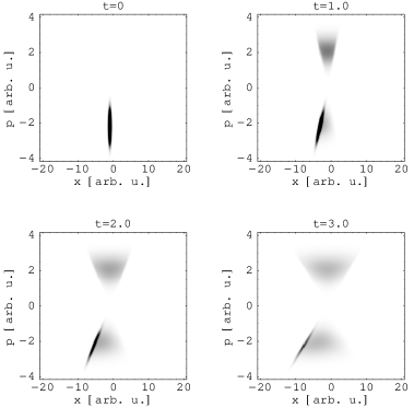
Figure 7: Snapshots of four stages of the temporal evolution of a Wigner distribution only subject to static roughness and vanishing external force. The underlying dataset is the same as the one used for figure 6 and 8.

In figure 6, we compare these results to a numerical solution of the transport equation without external force. The predictions (31) for the average position and (32) for the spatial width show a quite good agreement especially for the average position. The transient regime that is responsible for equilibration of the velocity classes however is not captured by the analytical solution and thus the spatial width is only a good estimate for the numerical solution, but definitely both exhibit the predicted linear behaviour. Figure 7 shows the dynamical evolution of the Wigner distribution, illustrating the growth of momentum classes with opposite signs.

The structure of the Wigner distribution in phase space when the second momentum class builds up also modifies the spatially averaged coherence function (16) as can be seen in figure 8. Since the scattering conserves energy, the momentum width of the cloud and hence the spatial coherence length remain constant in time, in distinction to the inelastic scattering shown in fig.3. The oscillations of the coherence function are a reminiscence of the standing wave formed by the two velocity classes. Note, however, that this interference is ‘classical’ in the sense that the Wigner function is positive all over phase space in this case.

3 Conclusion

In this paper, a transport theory for matter wave transport in low-dimensional waveguides has been formulated and solved in a few interesting limiting cases. We have shown that the scattering from thermal magnetic near fields that ‘leak out’ of metallic microstructures at room temperature limits the coherence of a cold atomic cloud. After a few scattering times, the spatial coherence of the ensemble gets reduced to the correlation length of the magnetic noise. This length scale is typically comparable to the distance of the waveguide to the metallic structures. Our results indicate that decoherence may be reduced by working with smaller metallic structures, reducing their temperature and their specific conductivity. Hopefully, a reasonable compromise between these conflicting requirements may be found.

The decoherence rates obtained in the present framework are quite large and should give rise to measurable effects when interference experiments with trapped matter waves are performed. From the theoretical point of view, it is imperative to generalize the transport theory to Bose-condensed samples: the transport equation then becomes nonlinear, and the potential fluctuations may expel particles out of the condensate. This issue is currently under study and results will be reported elsewhere. Finally, it is well known that in one dimension, static noise suppresses spatial diffusion, leading to Anderson localisation Anderson58 . This effect is beyond the scope of the present (semiclassical) theory, and its observation in atomic waveguides would be a clear manifestation of quantum-mechanical interference in multiple scattering.

Acknowledgments.

We thank F. Spahn, A. Pikovsky, and A. Demircan for interesting exchanges on the one-dimensional transport equation and S. A. Gardiner and A. Albus for useful discussions on extensions to Bose-condensed samples. C. H. acknowledges M. Wilkens for continuous support. S. P. was supported in part by the Office of Naval Research Research Contract No. 14-91-J1205, the National Science Foundation Grant PHY98-01099, the US Army Research Office and the Joint Services Optics Program.

Appendix A Low-frequency magnetic noise

As outlined in subsec. 1.2, we model the thermal excitations of the metallic structure by currents with a correlation function

$$\langle{j}_{i}^{*}({\bf x}_{1};\omega){j}_{j}({\bf x}_{2};\omega^{\prime})\rangle=$$

$$4\pi\hbar\varepsilon_{0}\omega^{2}\bar{n}(\omega)\,\delta_{ij}\,\delta(\omega-\omega^{\prime}){\rm Im}\,\varepsilon({\bf x}_{1})\,\delta({\bf x}_{1}-{\bf x}_{2}),$$ (33)

where $\bar{n}(\omega)$ is the Bose-Einstein occupation number. The current correlation is $\delta$-correlated in space provided the dielectric function is local. In the magnetostatic approximation, the vector potential generated by the currents is given by (in SI units)

$${\bf A}({\bf x};\omega)=\frac{\mu_{0}}{4\pi}\int\!{\rm d}^{3}x^{\prime}\,\frac{{\bf j}({\bf x}^{\prime};\omega)}{|{\bf x}-{\bf x}^{\prime}|}.$$ (34)

The cross correlation tensor of the vector potential is then simply obtained from the thermal average of ${\bf A}_{i}^{*}({\bf x}_{1};\omega){\bf A}_{j}({\bf x}_{2};\omega^{\prime})$. Taking the curl with respect to both ${\bf x}_{1}$ and ${\bf x}_{2}$, we get the magnetic cross correlation tensor:

$$\langle B_{i}^{*}({\bf x}_{1},\omega)B_{j}({\bf x}_{2},\omega^{\prime})\rangle=$$

$$\qquad=2\pi\delta(\omega-\omega^{\prime})B_{ij}({\bf x}_{1},{\bf x}_{2};\omega),$$ (35)

$$B_{ij}({\bf x}_{1},{\bf x}_{2};\omega)=S_{B}^{(bb)}(\omega)\frac{3\,{\rm Im}\,\varepsilon}{4\pi\omega/c}Y_{ij},$$ (36)

$$Y_{ij}=\left(\delta_{ij}{\rm tr}\,(X_{ij})-X_{ij}\right),$$ (37)

$$X_{ij}=\int_{V}\!{\rm d}^{3}x^{\prime}\,\frac{({\bf x}_{1}-{\bf x}^{\prime})_{i}({\bf x}_{2}-{\bf x}^{\prime})_{j}}{|{\bf x}_{1}-{\bf x}^{\prime}|^{3}|{\bf x}_{2}-{\bf x}^{\prime}|^{3}}.$$ (38)

We have normalized the spectral density to Planck’s blackbody formula

$$S_{B}^{(bb)}=\frac{\hbar\omega^{3}}{3\pi\varepsilon_{0}c^{5}({\rm e}^{\hbar\omega/k_{\rm B}T}-1)}.$$ (39)

The integration in (38) runs over the volume $V$ occupied by the thermal currents (where the imaginary part of $\varepsilon({\bf x}^{\prime},\omega)$ is nonzero). Putting ${\bf x}_{1}={\bf x}_{2}={\bf x}$ and using the scattering rate (1), we find from (36) that the scattering rate is of the form (2).

For homogeneous metallic structures, the dielectric function is $\varepsilon({\bf x}^{\prime},\omega)={\rm i}/(\varepsilon_{0}\varrho\omega)$ where $\varrho$ is the dc conductivity. In addition, the relevant frequencies are so low that the high-temperature limit of the Planck function is applicable. The prefactor in (36) then approaches the constant value

$$\omega\to 0:\quad S_{B}^{(bb)}(\omega)\frac{3\,{\rm Im}\,\varepsilon}{4\pi\omega/c}\to\frac{k_{\rm B}T}{4\pi^{2}\varepsilon_{0}^{2}c^{4}\varrho},$$ (40)

and we find the prefactor in (3). We have compared the results of the magnetostatic approximation to exact calculations using the retarded Green function for a layered medium. Both calculations agree in the short-distance limit where the distances are small compared to both the wavelength and the skin depth $\delta=\sqrt{2\varepsilon_{0}\varrho/(\omega c^{2})}$. However, the magnetostatic approximation overestimates the field components parallel to the layer by a factor of three. This is related to the fact that the noise currents (33) are not divergence-free at the surface. Possible improvements will be discussed elsewhere in more detail.

Figure 1: Scattering rate in a waveguide at distance $z$ from three metallic structures: half-space, thin layer, thin wire. The dashed line gives the large-distance limit (7) for the wire. The metal is copper at room temperature. Both the layer and the wire have a thickness $1\,\mu$m.

Figure 2: Spatial (normalized) correlation function of the thermal magnetic near field above a metallic surface at frequency $\omega/2\pi=30\,$MHz (copper at 300 K). The separation $s$ gives the distance between two observations points at the same height $z$ above the surface. Dots: exact evaluation, solid lines: asymptotic expansions in the short-distance regime, discussed in Henkel00b . For lower frequencies, the correlation function remains essentially unchanged.

Figure 3: Illustration of spatial decoherence in an atomic wave guide. The spatially averaged coherence function $\Gamma({\bf s},t)$ is plotted vs. the separation ${\bf s}$ for a few times $t$. Space is scaled to the field correlation length $l_{c}$ and time to the scattering time $1/\gamma$. A Lorentzian correlation function for the perturbation is assumed.

Figure 4: Numerical calculation of the temporal evolution of an atomic cloud in a one-dimensional waveguide. The cloud is subject to a positive external force and elastic scattering by a static rough potential, with a negative initial average velocity. The two lower curves in the left graph show the evolution of the average position $\langle x(t)\rangle$ determined numerically (solid line) and the ballistic short time behaviour (dotted line). The upper left curve displays the simulated variance $\langle\delta x^{2}(t)\rangle$ of the width in position space. The two lower curves on the right are the numerical values (solid line) for the average momentum $\langle p(t)\rangle$ of the cloud and the according short time ballistic acceleration (dotted line). The upper curve on the right illustrates the numerically computed width in momentum space $\langle\delta p^{2}(t)\rangle$.
The scattering rate is taken as $\gamma(p)=\gamma_{0}{\rm e}^{-|p|l_{c}}$ with $l_{c}=0.1\,$units, $\gamma_{0}=1\,$unit.

Figure 6: A free evolving Wigner distribution subject to elastic scattering, the distribution having initially a negative average velocity. The two lower curves show the evolution of the average position $\langle x(t)\rangle$ determined numerically (solid line) and from the analytical solution (31) (dotted line), whereas the upper curves displays the numerical average width $\langle\delta x^{2}(t)\rangle$ of the distribution (solid line) and its analytical estimate from (32) (dotted line).

Figure 8: Illustration of spatial decoherence in an atomic wave guide, caused by elastic scattering due to static roughness (no external force). The spatially averaged coherence function $\Gamma({\bf s},t)$ is plotted vs. the separation ${\bf s}$ for a few times $t$. Space is scaled to the field correlation length $l_{c}$ and time to the scattering time $1/\gamma_{0}=1/\gamma(0)$. The curves were extracted from the dataset underlying also figure 6.

References

- (1) J. Schmiedmayer: Phys. Rev. A 52, R13 (1995)
- (2) H. Ito, T. Nakata, K. Sakaki, M. Ohtsu, K. I. Lee, W. Jhe: Phys. Rev. Lett. 76, 4500 (1996)
- (3) H. Gauck, M. Hartl, D. Schneble, H. Schnitzler, T. Pfau, J. Mlynek: Phys. Rev. Lett. 81, 5298 (1998)
- (4) J. Denschlag, D. Cassettari, J. Schmiedmayer: Phys. Rev. Lett. 82, 2014 (1998) [quant-ph/9809076]
- (5) M. Key, I. G. Hughes, W. Rooijakkers, B. E. Sauer, E. A. Hinds, D. J. Richardson, P. G. Kazansky: Phys. Rev. Lett. 84, 1371 (2000)
- (6) D. Müller, D. Z. Anderson, R. J. Grow, P. D. D. Schwindt, E. A. Cornell: Phys. Rev. Lett. 83, 5194 (1999)
- (7) R. Folman, P. Krüger, D. Cassettari, B. Hessmo, T. Maier, J. Schmiedmayer: Phys. Rev. Lett. 84, 4749 (2000) [quant-ph/9912106]
- (8) N. H. Dekker, C. S. Lee, V. Lorent, J. H. Thywissen, S. P. Smith, M. Drndić, R. M. Westervelt, M. Prentiss: Phys. Rev. Lett. 84, 1124 (2000)
- (9) D. Cassettari, B. Hessmo, R. Folman, T. Maier, J. Schmiedmayer, submitted for publication [quant-ph/0003135]
- (10) M. Hammes, D. Rychtarik, V. Druzhinina, U. Moslener, I. Manek-Hönninger, R. Grimm: submitted for publication in J. mod. Optics (2000), special issue Fundamentals of Quantum Optics V, edited by F. Ehlotzky [physics/0005035]
- (11) C. Henkel, M. Wilkens: Europhys. Lett. 47, 414 (1999) [quant-ph/9902009]
- (12) C. Henkel, S. Pötting, M. Wilkens: Appl. Phys. B 69, 379 (1999) [quant-ph/9906128]
- (13) C. Henkel, K. Joulain, R. Carminati, J.-J. Greffet, “Spatial coherence of thermal near fields,” submitted for publication in Opt. Commun. (2000).
- (14) E. M. Lifshitz: Soviet Phys. JETP 2, 73 (1956) [J. Exper. Theoret. Phys. USSR 29, 94 (1955)]
- (15) T. Varpula, T. Poutanen: J. Appl. Phys. 55, 4015 (1984)
- (16) T. Gruner, D.-G. Welsch: Phys. Rev. A 53, 1818 (1996)
- (17) H. T. Dung, L. Knöll, D.-G. Welsch: Phys. Rev. A 57, 3931 (1998)
- (18) S. Scheel, L. Knöll, D.-G. Welsch: Phys. Rev. A 58, 700 (1998)
- (19) O. D. Stefano, S. Savasta, R. Girlanda: Phys. Rev. A 61, 023803 (2000)
- (20) S. M. Barnett: in Quantum fluctuations, Les Houches, Session LXIII, 1995, edited by S. Reynaud, E. Giacobino, J. Zinn-Justin. Amsterdam: Elsevier 1997, pp. 137–179
- (21) C. Kittel: Introduction to Solid State Physics, 5th ed.. New York: Wiley 1976
- (22) L. Ryzhik, G. Papanicolaou, J. B. Keller: Wave Motion 24, 327 (1996)
- (23) C. Henkel, K. Mølmer, R. Kaiser, N. Vansteenkiste, C. I. Westbrook, A. Aspect: Phys. Rev. A 55, 1160 (1997)
- (24) Y. B. Ovchinnikov, I. Manek, R. Grimm: Phys. Rev. Lett. 79, 2225 (1997)
- (25) P. W. Anderson: Phys. Rev. 109, 1492 (1958)