Three-party entanglement from positronium
Abstract
The decay of ortho-positronium into three photons produces a physical realization of a pure state with three-party entanglement. Its quantum correlations are analyzed using recent results on quantum information theory, looking for the final state which has the maximal amount of GHZ-like correlations. This state allows for a statistical dismissal of local realism stronger than the one obtained using any entangled state of two spin one-half particles.
pacs:
PACS Nos. 03.65.Bz, 03.67.-a, 12.20.-mI Introduction
Entanglement or quantum correlations between many space-separated subsystems has been recognized as one of the most intrinsic properties of quantum mechanics and provides the basis for many genuine applications of quantum information theory. It is, then, quite natural to look for physical situations in which quantum entangled states are obtained. Most of the theoretical and experimental effort has so far been devoted to unveil physical realizations of quantum states describing two quantum correlated subsystems. The search for physical systems displaying clean three-party entanglement is not simple. In this paper, we shall analyze decays of particles as a natural scenario for fulfilling such a goal. More precisely, we shall show that the decay of ortho-positronium into three photons corresponds to a highly entangled state. Let us now review what entanglement can be used for and why it is interesting to look for quantum correlation between more than two particles.
In 1935 Einstein, Podolsky and Rosen [1], starting from three reasonable assumptions of locality, reality and completeness that every physical theory must satisfy, argued that quantum mechanics (QM) is an incomplete theory. They did not question quantum mechanics predictions but rather quantum mechanics interpretation [2]. Their argument was based on some inconsistencies between quantum mechanics and their local-realistic premises (LR) which appear for quantum states of bipartite systems, . It was in 1964 when Bell [3] showed that any theory compatible with LR assumptions can not reproduce some of the statistical predictions of QM, using a gedankenexperiment proposed in [4] with two quantum correlated spin- particles in the singlet state
| (1) |
In his derivation, as it is well-known, quantum correlations or entanglement have a crucial role. Actually, the singlet state is known to be the maximally entangled state between two particles. The conflict between LR and QM arises since the latter violates some experimentally verifiable inequalities, called Bell inequalities, that any theory according to the local-realistic assumptions ought to satisfy. It is then possible to design real experiments testing QM against LR (for a detailed discussion see [5]). Correlations of linear polarizations of pair of photons were measured in 1982 showing strong agreement with quantum mechanichs predictions and violating Bell inequalities [6]. Nowadays, Bell inequalities have been tested thoroughly in favor of QM [7].
More recently, it has been pointed out that some predictions for quantum systems having quantum correlations between more than two particles give a much stronger conflict between LR and QM than any entangled state of two particles. The maximally entangled state between three spin- particles, the so-called GHZ (Greenberger, Horne and Zeilinger) state [8]
| (2) |
shows some perfect correlations incompatible with any LR model (see [2] and also [9] for more details). It is then of obvious relevance to obtain these GHZ-like correlations. Producing experimentally a GHZ state has turned out to be a real challenge yet a controlled instance has been produced in a quantum optics experiment [10].
Entanglement is then important for our basic understanding of quantum mechanics. Recent developments on quantum information have furthermore shown that it is also a powerful resource for quantum information applications. For instance, teleportation [11] uses entanglement in order to obtain surprising results which are impossible in a classical context. A lot of work has been performed trying to know how entanglement can be quantified and manipulated. Our aim in this paper consists on looking for GHZ-like correlations, which are truly three-party pure state entanglement, in the decay of ortho-positronium to three photons. The choice of this physical system has been motivated mainly by several reasons. First, decay of particles seems a very natural source of entangled particles. Indeed, positronium decay to two photons was one of the physical systems proposed long time ago as a source of two entangled space-separated particles [12]. On a different line of thought, some experiments for testing quantum mechanics have been recently proposed using correlated neutral kaons coming from the decay of a -meson [13]. In the case of positronium, three entangled photons are obtained in the final state, so it offers the opportunity of analyzing a quantum state showing three-party correlations similar to other experiments in quantum optics.
The structure of the paper goes as follows. We first review the quantum states emerging in both para- and ortho-positronium decays. Then, we focus on their entanglement properties and proceed to a modern analysis of the three-photon decay state of ortho-positronium. Using techniques developed in the context of quantum information theory, we show that this state allows in principle for an experimental test of QM finer than the ones based on the use of the singlet state. We have tried to make the paper self-contained and easy to read for both particle physicists and quantum information physicists. The first ones can found a translation of some of the quantum information ideas to a well-known situation, that is, the positronium decay to photons, while the second ones can see an application of the very recent techniques obtained for three-party entangled states, which allow to design a QM vs LR test for a three-particle system in a situation different from the GHZ state.
II Positronium decays
A Positronium properties
Let us start reminding some basic facts about positronium. Positronium corresponds to a bound state. These two spin- particles can form a state with total spin equal to zero, para-positronium (p-Ps), or equal to one, ortho-positronium (o-Ps). Depending on the value of its angular momentum, it can decay to an even or an odd number of photons as we shall see shortly.
Positronium binding energy comes from the Coulomb attraction between the electron and the positron. In the non-relativistic limit, its wave function is [14]
| (3) |
where , i.e. twice the Bohr radius of atomic hydrogen, and is the electron mass. Note that the wave function takes significant values only for three-momenta such that , which is consistent with the fact that the system is essentially non-relativistic.
The parity and charge conjugation operators are equal to
| (4) |
where and are the orbital and spin angular momentum. Positronium states are then classified according to these quantum numbers so that the ground states are , with , for the p-Ps and , having , for the o-Ps.
Positronium is an unstable bound state that can decay to photons. Since a -photon state transforms as under charge conjugation, which is an exact discrete symmetry for any QED process such as the decay of positronium, we have that the ground state of p-Ps (o-Ps) decays to an even (odd) number of photons [15]. The analysis of the decay of positronium to photons can be found in a standard QED textbook [14]. Para-positronium lifetime is about 0.125 ns, while for the case of ortho-positronium the lifetime is equal to approximately 0.14 s [16].
The computation of positronium decays is greatly simplified due to the following argument. The scale which controls the structure of positronium is of the order of . On the other hand, the scale for postrinomium annihilation is of the order of . Therefore, it is easy to prove that positronium decays are only sensitive to the value of the wave function at the origin. As a consequence, it is possible to factor out the value of the wave function from the tree-level QED final state computation [14]. A simple computation of Feymann diagrams will be enough to write the precise structure of momenta and polarizations which describe the positronium decays. Furthermore, only tree-level amplitudes need to be computed since higher corrections are suppressed by one power of . Let us now proceed to analyze the decays of p-Ps and o-Ps in turn.
B Para-positronium decay
Para-positronium ground state decays into two photons. Because of the argument mentioned above, the determination of the two-photon state coming from the p-Ps decay is simply given by the lowest order Feynmann diagram of . Since positronium is a non-relativistic particle to a very good approximation, the three-momenta of and are taken equal to zero, and the corresponding spinors are replaced by a two-component spin. This implies that the tree-level calculation of the annihilation of p-Ps into two photons is equal to, up to constants,
| (5) |
where (see [14] for more details) is the two-component spinor describing the fermions, , and gives
| (6) |
where stands for the circular polarization vector associated to the outgoing photon and is the identity matrix. More precisely, for a photon having the three-momentum vector , the polarization vectors can be chosen
| (7) |
where and they obey
| (8) | |||
| (9) |
From the expressions of the polarizaton vectors and the three-momentum and energy conservation, it follows that the scalar term is
| (10) |
and it verifies
| (11) | |||
| (12) |
The two fermions in the para-positonium ground state are in the singlet state, , and then, using the previous relations for and (5), the two-photon state resulting of the p-Ps desintegration is
| (13) |
The two-photon state resulting from p-Ps decay is thus equivalent to a maximally entangled state of two spin- particles. This is a well-known result and was, actually, one of the physical system first proposed as a source of particles having the quantum correlations needed to test QM vs LR [12].
C Ortho-positronium decay
The ground state of ortho-positronium has and, due to the fact that charge conjugation is conserved, decays to three photons. Repeating the treatment performed for the p-Ps annihilation, the determination of the three-photon state resulting from the o-Ps decay requires the simple calculation of the tree-level Feynmann diagrams corresponding to . Its tree-level computation gives, up to constants,
| (14) |
and the matrix is equal to [14]
| (15) |
where
| (16) |
Using (8) we can rewrite in the following way
| (17) |
where
| (20) | |||||
Notice that the helicity coefficient for the cyclic permutations of explicitly enforces the vanishing of the and polarizations,
| (21) |
On the other hand, the rest of structures are different from zero
| (22) | |||
| (23) |
and similar expressions for the other cyclic terms.
The original in the ortho-positronium could be in any of the three triplet states. It can be shown, using (14) and (17), that when the initial positronium state is , the decay amplitude is proportional to , while the same argument gives for and for . Now, considering the explicit expressions of the polarization vectors (7), with without loss of generality, and (22), it is easy to see that the three-photon state coming from the o-Ps decay is, up to normalization,
| (24) | |||||
| (25) | |||||
| (26) |
when the third component of the ortho-positronium spin, , is equal to zero, and
| (27) | |||||
| (28) | |||||
| (29) |
when .
The final state of the o-Ps decay is, thus, an entangled state of three photons, whose quantum correlations depend on the angles among the momenta of the outgoing three photons. For the rest of the paper we will consider the first family of states () although equivalent conclusions are valid for the second one. In the next sections we will analyze the entanglement properties of the states , using some of the quantum information techniques and comparing them to the well-known cases of the singlet and GHZ state.
III Entanglement properties
The quantum correlations of the three-photon entangled state obtained from the o-Ps annihilation depend on the position of the photon detectors, i.e. on the photon directions we are going to measure. Our next aim will be to choose from the family of states given by (24) the one that, in some sense, has the maximum amount of GHZ-like correlations. In order to do this, we first need to introduce some recent results on the study of three-party entanglement.
The set of states form a six-parameter dependent family in the Hilbert space , so that each of its components is equivalent to a state describing three spin- particles or three qubits (a qubit, or quantum bit, is the quantum version of the classical bit and corresponds to a spin- particle). Two pure states belonging to a generic composite system , i.e. parties each having a -dimensional Hilbert space, are equivalent as far as their entanglement properties go when they can be transformed one into another by local unitary transformations. This argument gives a lower bound for the entanglement parameters a generic state depends on. Since the number of real parameters for describing it is , and the action of an element of the group of local unitary transformations is equivalent to the action of , which depends on real parameters, the number of entanglement parameters is bounded by . For our case this counting of entanglement parameters gives six, since we have , and it can be proved that this is indeed the number of nonlocal parameters describing a state in [17].
The above arguments imply that six independent quantities invariant under the action of the group of local unitary transformations will be enough, up to some discrete symmetry, to describe the entanglement properties of any three-qubit pure state. Given a generic state
| (30) |
where are the elements of a basis in each subsystem, A, B and C, the application of three local unitary transformations , and transforms the coefficients into
| (31) |
From this expression it is not difficult to build polynomial combinations of the coefficient which are invariant under local unitary transformations [17, 18]. These quantities are good candidates for being an entanglement parameter. For example, one of these invariants is
| (32) |
where is the density matrix describing the local quantum state of A (and the same happens for B and C). In [18] the six linearly independent polynomial invariants of minor degree were found (a trivial one is the norm) and a slightly modified version of these quantities was also proposed in [19]. In the rest of the paper we will not consider the norm, so the space of entanglement parameters of the normalized states belonging to has dimension equal to five.
A particularly relevant polynomial invariant is the so-called tangle, , introduced in [20]. There is strong evidence that somehow it is a measure of the amount of “GHZ-ness” of a state [19, 20, 21, 22]. It corresponds to the modulus of the hyperdeterminant of the hypermatrix given by the coefficients [23], which from (30) corresponds to
| (33) |
where and . This quantity can be shown to be symmetric under permutation of the indices .
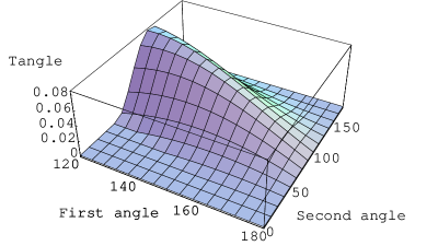
Because of the interpretation of the tangle as a measure of the GHZ-like correlations, we will choose the position of the photon detectors, from the set of states (24), the ones that are associated to a maximum tangle. In the figure 1 it is shown the variation of the tangle with the position of the detectors. It is not difficult to see that the state of (24) with maximum tangle corresponds to the case , i.e. the most symmetric configuration, that we shall call “Mercedes-star” geometry. The normalized state obtained from (24) for this geometry is
| (34) |
Note that the GHZ state has tangle equal to , while the value of the tangle of (34) is lower,
| (35) |
It is arguable that a “Mercedes-star” geometry was naturally expected to produce a maximum tangle state. Indeed, GHZ-like quantum correlations do not singularize any particular qubit.
Let us also mention that the state we have singled out has some nice properties from the point of view of group theory. It does correspond to the sum of two of the elements of the coupled basis resulting from the tensor product of three spin- particles, , [24]
| (36) |
where
| (37) | |||
| (38) |
The quantum correlations of (34) will be now analyzed.
IV Useful decompositions
In this section, the state (34) will be rewritten in some different forms that will help us to understand better its nonlocal properties. First, let us mention that for any generic three-qubit pure state and by performing change of local bases, it is possible to make zero at least three of the coefficients of (30) [19, 25]. A simple counting of parameters shows that this is in fact the expected number of zeros. This means that by a right choice of the local bases, any state can be written with the minimum number of coefficients , i.e. we are left with all the non-local features of the state, having removed all the “superfluous” information due to local unitary tranformations. For the case of the state (34) it is easy to prove [26] that it can be expressed as
| (39) |
which is the minimum decomposition in terms of product states built from local bases (four of the coefficients are made equal to zero).
An alternative decomposition, that will prove to be fruitful for the rest of the paper, consists of writing the state as a sum of two product states. This decomposition is somewhat reminiscent of the form of the GHZ state, which is a sum of just two product states, and is only possible when the tangle is different from zero [19, 21] as it happens for our state (see 35). The state then can be written as
| (41) | |||||
where and . We omit the details for the explicit computation of this expression since they can be found in [19, 21]. It is worth noticing that o-Ps decay is hereby identified to belonging to an interesting type of states already classified in quantum information theory [21].
The above decomposition allows for an alternative interpretation of the initial state as an equally weighted sum of two symmetric product states. Note that the Bloch vector, , representing the first local spinor appearing in (41) is pointing to the axis, i.e. , while the second is located in the plane with an angle of 120∘ with the axis, i.e. . By performing a new unitary transformation, (41) can be written as
| (42) |
where . Now, the two Bloch vectors are in the plane, pointing to the and directions. The GHZ state corresponds to the particular case and .
V Quantum mechanics vs local realism
The quantum correlations present in some three-qubit pure states show, as it was mentioned in the introduction, a much stronger disagreement with the predictions of a local-realistic model than any two-qubit entangled state. In fact, contrary to the case of the singlet state, no LR model is able to reproduce all the perfect correlations predicted for the maximally entangled state of three qubits [2]. The state (34) emerging from o-Ps decay is not a GHZ state, although it has been chosen the one with the maximum tangle in order to maximize GHZ-like correlations. In this section we will show how to use it for testing quantum mechanics against local-realistic models, and then we will compare its performance against existing tests for the maximally entangled states of two and three spin- particles. We start reviewing some of the consequences derived from the arguments proposed in [1].
A QM vs LR conflict
Given a generic quantum state of a composite system shared by parties, there should be an alternative LR theory which reproduces all its statistical predictions. In this LR model, a state denoted by will be assigned to the system specifying all its elements of physical reality. In particular, the result of a measurement depending on a set of parameters performed locally by one of the parties, say A, will be specified by a function . The same will happen for each of the space-separated parties and, since there is no causal influence among them, the result measured on A can not modify the measurement on B. For example, if the measurement is of the Stern-Gerlach type, the parameters labeling the measurement are given by a normalized vector and are the LR functions describing the outcome.
The LR model can be very general provided that some conditions must be satisfied. Consider a generic pure state belonging to shared by three observers A, B and C, which are able to perform Stern-Gerlach measurements in any direction. Since the outcomes of a Stern-Gerlach measurement are only , it is easy to check that for any pair of measurements on each subsystem, described by the LR functions and , and , and , and for all their possible values, it is always verified
| (43) |
It follows from this relation that
| (44) |
This constraint is known as Mermin inequality [27] and has to be satisfied by any LR model describing three space-separated systems.
Let us now take the GHZ state (2). It is quite simple to see that if the observables and are equal to and (the same for parties B and C), the value of (44) is , so an experimental condition is found that allows to test quantum mechanics against local realism. Note that this is the maximal violation of inequality (44). Moreover, the GHZ state also satisfies that and no LR model is able to take into account this perfect correlation result because of (43) [2]. This is a new feature that does not appear for the case of a two maximally entangled state of two spin- particles. In this sense it is often said that a most dramatic contrast between QM and LR emerges for entanglement between three subsystems.
Let us go back to the state given by the ortho-positronium decay (34). Our aim is to design an experimental situation where a conflict between QM and LR appears, so we will look for the observables that give a maximal violation of (44). Such observables will extremize that expression. Using the decomposition (42), the expectation value of three local observables is
| (45) | |||||
| (46) | |||||
| (47) |
where and . Because of the symmetry of the state under permutation of parties, the Stern-Gerlach directions are taken satisfying and . Substituting this expression in (44), we get the explicit function to be extremized. For the case of the GHZ state described above, the extreme values were obtained using two observables with , i.e. in the plane. Since (42) is the GHZ-like decomposition of the initial state, we take and it is easy to check that in this case . Mantaining the parallelism with the GHZ case, it can be seen that all the partial derivatives vanish when it is also imposed and . In our case the calculation of (44) gives , so a conflict between local-realistic models and quantum mechanics again appears, and then the three-photon state coming from the ortho-positronium decay can be used, in principle, to test QM vs LR with the set of observables given by the normalized vectors
| (48) |
There is an alternative set of angles and that makes zero all the partial derivatives of : the combination of local observables (44) is equal to for
| (49) |
This second set of parameters will be seen to produce in the end a weaker dismissal of LR.
Our next step will be to carry over the comparison of this QM vs LR test against the existent ones for the maximally entangled states of three and two spin- particles, i.e. the GHZ and singlet state. It is quite evident that the described test should be worse than the obtained for the GHZ state. It is less obvious how this new situation will compare with the singlet case.
B Comparison with the maximally entangled states of two and three spin- particles
We will now estimate the “strength” of the QM vs LR test proposed above, being this “strength” measured by the number of trials needed to rule out local-realism at a given confidence level, as Peres did in [28]. A reasoning anologous to the one given in [28] will be done here for the state (34) and the observables (48).
Imagine a local-realistic physicist who does not believe in quantum mechanics. He assigns prior subjective probabilities to the validity of LR and QM, and , expressing his personal belief. Take for instance . His LR theory is not able to reproduce exactly all the QM statistical results of some quantum states. Consider the expectation value of some observable with two outcomes such that is predicted for some quantum state, while LR gives . Since the value of the two possible outcomes are , the probablity of having is for QM and for LR. An experimental test of the observable now is performed times yielding times the result . The prior probabilities and are modified according to the Bayes theorem and their ratio has changed to
| (50) |
where
| (51) |
is the LR probability of having times the outcome , and we have the same for , being replaced by . Following Peres [28], the confidence depressing factor is defined
| (52) |
which accounts for the change in the ratio of the probabilities of the two theories, i.e. it reflects how the LR belief changes with the experimental results. Like in a game, our aim is to destroy as fast as we can the LR faith of our friend by choosing an adequate experimental situation. It can be said, for example, that he will give up when, for example, . Since the world is quantum, , and the number of experimental tests needed to obtain is equal to
| (53) |
being the information distance [29] between the QM and LR binomial distribution for the outcome . The more separate the two probability distributions are, measured in terms of the information distance, the fewer the number of experiments is.
Let us come back to the three-party entangled state coming from the ortho-positronium decay (34) under the local measurements described by (48). As it has been shown above, a contradiction with any LR model appears for the combination of the observables given by the Mermin inequality. In our case quantum mechanics gives the following predictions
| (54) |
and this implies that and . This is the QM data that our LR friend has to reproduce as well as possible. Because of the symmetry of the state he will assign the same probability to the events , and and to . However, his model has to satisfy the constraint given by (44), so the best he can do is to saturate the bound and then
| (55) |
Now, according to the probabilities and his LR model predicts, we choose the experimental test that minimizes (53), i.e. we consider the event () when (), and the experimental results will destroy his LR belief after () trials. The best value our LR friend can assign to is the solution to
| (56) |
with the constraint (55), and this condition means that and trials are needed to have a depressing factor equal to . Repeating the same calculation for the observables giving by (49), the number of trials slightly increases, , despite of the fact that the violation of the inequality is greater than the obtained for (48).
In ref. [28] the same reasoning was applied to the maximally entangled state of two and three spin- particles, showing that in the first case, and for the latter (see table I). Our result then implies that the three-photon entangled state produced in the ortho-positronium decay has, in some sense, more quantum correlations than any entangled state of two spin- particles.
C Generalization of the results
It is easy to generalize some of the results obtained for the entangled state resulting from the o-Ps decay. As it has been mentioned, this state can be understood as an equally weighted sum of two symmetric product states, since it can be written as (42). The Bloch vectors of the two local states appearing in this decomposition form an angle of . It is clear that the conclusions seen above depend on the angle between these vectors, i.e. with their degree of non-orthogonality. The family of states to be analyzed can be parametrized in the following way
| (57) |
where is the angle between the two local Bloch vectors, and and is a positive number given by the normalization of the state. An alternative parametrization of this family is, using (39) and defining ,
| (58) |
The expectation value of three local observables for this set of states follows trivially from (45). Using this expression it is easy to see that the combination of the expectation values of (44) has all the partial derivatives equal to zero for the set of observables given in (48) independently of . For these observables, the dependence of expression (44) with the degree of orthogonality between the two product states is given in figure 2. There is no violation of the Mermin inequality for the case in which . In this situation one can always found a LR model able to reproduce the QM statistical prediction given by (44) and the observables (48). We can now repeat all the steps made in order to determine the number of trials needed to rule out local realism as a function of the angle . In figure 3 we have summaryzed the results. We have shown only the cases where the number of trials is minor than two hundred, since this is the value obtained for the singlet. Note that the case , which corresponds to (34), is very close to the region where there is no improvement compared to the maximally entangled state of two qubits.
All these results can be understood in the following way: the smaller the angle between the two local states, , the higher the overlap of the state with the product state having each local Bloch vector pointing in the direction of the axis, which corresponds to the state in (58). This means that the quantum state we are handling is too close to a product state [25], and thus, no violation of the Mermin inequality can be observed.
VI Concluding remarks
In this work we have analyzed the three-particle quantum correlations of a physical system given by the decay of the ortho-positronium into a three-photon pure state. After obtaining the state describing the polarization of the three photons (34), some of the recent techniques developed for the study of three-party entanglement have been applied. The particular case where the three photons emerge in a symmetric, Mercedes-star-like configuration, corresponds to the state with the maximum tangle. We have shown that this state allows a priori for a QM vs LR test which is stronger than any of the existing ones that use the singlet state. In this sense, ortho-positronium decays into a state which carries stronger quantum correlations than any entangled state of two spin- particles.
Bose symmetrization has played a somewhat negative role in reducing the amount GHZ-ness of the o-Ps decay state. Indeed, the natural GHZ combination emerging from the computation of Feynmann diagrams has been symmetrized due to the absence of photon tagging to our state , inducing a loss of tangle. The quantum optics realization of the GHZ state does avoid symmetrization through a geometric tagging [10]. It is, thus, reasonable to look for pure GHZ states in decays to distinct particles, so that tagging would be carried by other quantum numbers, as e.g. charge. It is, on the other hand, peculiar to note that symmetrization in the system is responsible for its entanglement () [13].
Finally, let us briefly discuss the experimental requirements needed for testing quantum mechanics as it has been described in this paper. In order to do this, the circular polarizations of the three photons resulting from an ortho-positronium decay have to be measured. The positions of the three detectors are given by the “Mercedes-star” geometry and their clicks have to detect the coincidence of the three photons. The energy of these photons is of the order of 1 Mev. Polarization analyzers with a good efficiency would allow us to acquire statistical data showing quantum correlations which would violate the Mermin inequality discussed above. Unfortunately, as far as we know, no such analizers exist for this range of energies. A possible way-out might be to use Compton scattering to measure the photon polarizations [30]. However, Compton effect just gives a statistical pattern depending on the photon and electron polarizations which is not a direct measurement of the polarizations. Further work is needed to modify our analysis of QM vs LR to accommodate for such indirect measurements.
Acknowledgments
We acknowledge J. Bernabeu for suggesting positronium as a source of three entangled particles and reading carefully the paper. We also thank A. Czarnecki, D. W. Gidley, M. A. Skalsey and V. L. Telegdi for comments about the measurement of the photon polarizations in the ortho-positronium decay. We acknowledge financial support by CICYT project AEN 98-0431, CIRIT project 1998SGR-00026 and CEC project IST-1999-11053, A. A. by a grant from MEC (AP98). Financial support from the ESF is also acknowledged. This work was concluded during the 2000 session of the Benasque Center for Science, Spain.
REFERENCES
- [1] A. Einstein, B. Podolsky and N. Rosen, Phys. Rev. 47 (1935), 777.
- [2] D. M. Greenberger, M. A. Horne, A. Shimony and A. Zeilinger, Am. J. Phys. 58 (1990), 1131.
- [3] J. S. Bell, Physics 1 (1964), 195.
- [4] D. Bohm and Y. Aharonov, Phys. Rev. 108 (1957), 1070.
- [5] J. F. Clauser and A. Shimony, Rep. Prog. Phys. 41 (1978), 1881.
- [6] A. Aspect, J. Dalibard and G. Roger, Phys. Rev. Lett. 49 (1982), 1804.
- [7] W. Tittel, J. Brendel, H. Zbinden and N. Gisin, Phys. Rev. Lett. 81 (1998), 3563; G. Weihs, T. Jennewein, C. Simon, H. Weinfurter and A. Zeilinger, Phys. Rev. Lett. 81 (1998), 5039.
- [8] D. M. Greenberger, M. A. Horne and A. Zeilinger, “Going beyond Bell’s theorem”, in Bell’s Theorem, Quantum Theory and Conceptions of the Universe, edited by M. Kafatos (Kluwer Academic, Dordrecht, The Netherlands, 1989), pp. 73-76.
- [9] N. D. Mermin, Am. J. Phys. 58 (1990), 731.
- [10] D. Bouwmeester, J. Pan, M. Daniell, H. Weinfurter and A. Zeilinger, Phys. Rev. Lett. 82 (1999), 1345, quant-ph/9810035.
- [11] C. H. Bennett, G. Brassard, C. Crépeau, R. Josza, A. Peres and W. K. Wootters, Phys. Rev. Lett. 70 (1993), 1895.
- [12] J. F. Clauser, M. A. Horne, A. Shimony and R. A. Holt, Phys. Rev. Lett. 23 (1969), 880.
- [13] See for instance A. Di Domenico, Nucl. Phys. B 450 (1995), 293; B. Ancochea, A. Bramon and M. Nowakowski, Phys.Rev. D 60 (1999), 094008, hep-ph/9811404; F. Benatti and R. Floreanini, Eur. Phys. J. C 13 (2000), 267, hep-ph/9912348.
- [14] C. Itzykson and J. Zuber, Quantum field theory, McGraw-Hill.
- [15] L. Wolfenstein and D. G. Ravenhall, Phys. Rev. 88 (1952), 279.
- [16] Andrzej Czarnecki, Acta Phys. Polon. B 30 (1999) 3837, hep-ph/9911455.
- [17] N. Linden and S. Popescu, Fortsch. Phys. 46 (1998), 567, quant-ph/9711016.
- [18] A. Sudbery, “On local invariants of pure three-qubit states”, quant-ph/0001116.
- [19] A. Acín, A. Andrianov, L. Costa, E. Jané, J.I. Latorre and R. Tarrach,“Schmidt decomposition and classification of three-quantum-bit states”, quant-ph/0003050, to appear in Phys. Rev. Lett..
- [20] V. Coffman, J. Kundu, W. K. Wootters, Phys. Rev. A 61 (2000), 052306, quant-ph/9907047.
- [21] W. Dür, G. Vidal and J. I. Cirac, “Three qubits can be entangled in two inequivalent ways”, quant-ph/0005115.
- [22] T. A. Brun and O. Cohen, “Parametrization and distillability of three-qubit entanglement”, quant-ph/0005124.
- [23] I. M. Gelfand, M. M. Kapranov and A. V. Zelevinsky, “Discriminants, resultants and multidimensional determinants”, Birkhäuser Boston 1994. Its explicit form is: .
- [24] S. Rai and J. Rai, “Group-theoretical Structure of the Entangled States of N Identical Particles”, quant-ph/0006107.
- [25] A. Higuchi and A. Sudbery, “How entangled can two couples get?”, quant-ph/0005013; H. A. Carteret, A. Higuchi and A. Sudbery, “Multipartite generalisation of the Schmidt decomposition”, quant-ph/0006125.
- [26] A. Acín, A. Andrianov, E. Jané, J. I. Latorre and R. Tarrach, in preparation.
- [27] N. D. Mermin, Phys. Rev. Lett. 65 (1990), 1838.
- [28] A. Peres, “Bayesian analysis of Bell inequalities”, quant-ph/9905084.
- [29] S. Kullback, Information theory and statistics, Wiley, New York (1959).
- [30] B. K. Arbic, S. Hatamian, M. Skalsey, J. Van House and W. Zheng, Phys. Rev. A 37 (1988), 3189.


| State | Number of trials | |
|---|---|---|
| GHZ | ||
| Positronium state (34) | ||
| Singlet |