Schrödinger-Cat Entangled State Reconstruction in the Penning Trap

Abstract

We present a tomographic method for the reconstruction of the full entangled quantum state for the cyclotron and spin degrees of freedom of an electron in a Penning trap. Numerical simulations of the reconstruction of several significant quantum states show that the method turns out to be quite accurate.

I Introduction

A single electron trapped in a Penning trap [1] is a unique quantum system in that it allows the measurement of fundamental physical constants with striking accuracy. Recently, the electron cyclotron degree of freedom has been cooled to its ground state, where the electron may stay for hours, and quantum jumps between adjacent Fock states have been observed [2]. It is therefore evident that the determination of the genuine (possibly entangled) quantum state of the trapped electron is an important issue, with implications in the very foundations of physics, and in particular of quantum mechanics. After the pioneering work of Vogel and Risken [3], several methods have been proposed in order to reconstruct the quantum state of light and matter [4], which range from quantum tomography [5] through quantum state endoscopy [6], to Wigner function determination from outcome probabilities [7]. Also, different techniques [8] have been proposed which allow to deal with entangled states.

In fact, entanglement [9] has been defined as one of the most puzzling features of quantum mechanics, and it is at the heart of quantum information processing. Some fascinating examples of the possibilities offered by sharing quantum entanglement are quantum teleportation [10, 11], quantum dense coding [12], entanglement swapping [13], quantum cryptography [14], and quantum computation [15]. A striking achievement in this field has been the recent entanglement of four trapped ions [16].

In the present work we propose to reconstruct the full entangled state (combined cyclotron and spin state) of an electron in a Penning trap by using a modified version of quantum state tomography. Previous proposals [17] need the a priori knowledge of the spin state and therefore are not able to deal with entangled states. Our method, on the contrary, has the ability of measuring the full (entangled) pure state of the two relevant degrees of freedom of the electron. In order to reach this scope, our method takes advantage of the magnetic bottle configuration to perform simultaneous measurements of the cyclotron excitation and of the $z$ component of the spin as a function of the phase of an applied driving electromagnetic field. The complete structure of the cyclotron-spin quantum state is then obtained with the help of a tomographic reconstruction from the measured data.

The present paper is organized as follows: In Sec. II we outline the basic model of an electron trapped in a Penning trap, while in Sec. III we describe the main idea of our reconstruction procedure. In Sec. IV and V we concentrate on the measurement of the spin and on the tomographic reconstruction of the cyclotron states, respectively. We present the results of our numerical simulations in Sec. VI, and conclude briefly in Sec. VII.

II The basic model

Let us consider the motion of an electron trapped by the combination of a homogeneous magnetic field ${\bf B}_{0}$ along the positive $z$ axis and an electrostatic quadrupole potential in the $xy$ plane, which is known as a Penning trap [1]. The corresponding Hamiltonian can be written as

$${\hat{H}}={1\over{2m}}\left[{\bf p}-{q\over c}{\bf A}\right]^{2}+{{qV_{o}}\over{2d^{2}}}\left({\hat{z}}{}^{2}-{{{\hat{x}}{}^{2}+{\hat{y}}{}^{2}}\over 2}\right)\;,$$ (1)

where ${\bf A}=(B_{o}y/2,-B_{o}x/2,0)$ is the vector potential, $c$ is the speed of light, $d$ characterizes the dimensions of the trap, $V_{o}$ is the electrostatic potential applied to its electrodes, and $q$ the electron charge.

The spatial part of the electronic wave function consists of three degrees of freedom, but neglecting the slow magnetron motion (whose characteristic frequency lies in the kHz region), here we only consider the axial and cyclotron motions, which are two harmonic oscillators radiating in the MHz and GHz regions, respectively. The spin dynamics results from the interaction between the magnetic moment of the electron and the magnetic field, so that the total quantum Hamiltonian is

$${\hat{H}}_{\rm tot}=\hbar{\omega_{z}}({{\hat{a}}^{\dagger}}_{z}{\hat{a}}_{z}+1/2)+\hbar{\omega_{c}}({{\hat{a}}^{\dagger}}_{c}{\hat{a}}_{c}+1/2)+{{\hbar{\omega_{s}}}\over 2}{\hat{\sigma}}_{z}\;.$$ (2)

In the previous expression we have introduced the lowering operator for the cyclotron motion

$${\hat{a}}_{c}={1\over 2}\left[{1\over{2\beta\hbar}}({\hat{p}}_{x}-i{\hat{p}}_{y})-i\beta({\hat{x}}-i{\hat{y}})\right]\;,$$ (3)

where $\beta=m{\omega_{c}}/2\hbar$ and ${\omega_{c}}=qB_{o}/mc$ is the resonance frequency associated to the cyclotron oscillation. For the axial motion we have

$${\hat{a}}_{z}=\left({{m{\omega_{z}}}\over{2\hbar}}\right)^{1/2}{\hat{z}}+i\left({1\over{2m\hbar{\omega_{z}}}}\right)^{1/2}\hat{p}_{z}\;,$$ (4)

where ${\omega_{z}}^{2}=qV_{o}/md^{2}$. In the last term of Eq. (2), ${\hat{\sigma}}_{z}$ is the Pauli spin matrix and ${\omega_{s}}=(g/2){\omega_{c}}$.

The obtained Hamiltonian (2) is then made of three independent terms. Even though the only physical observable experimentally detectable is the axial momentum ${\hat{p}}_{z}$, in the following both the cyclotron and spin states will be reconstructed. Considering the eigenstates of ${\hat{\sigma}}_{z}$

$$|\uparrow\rangle=\left(\begin{array}[]{c}1\\ 0\end{array}\right)\;,\qquad|\downarrow\rangle=\left(\begin{array}[]{c}0\\ 1\end{array}\right)\;,$$ (5)

we can write the most general pure state of the trapped electron in the form

$$|\Psi\rangle=c_{1}|\psi_{1}\rangle|\uparrow\rangle+c_{2}|\psi_{2}\rangle|\downarrow\rangle\;,$$ (6)

$|\psi_{1}\rangle$ and $|\psi_{2}\rangle$ being two unknown cyclotron states. The complex coefficients $c_{1}$ and $c_{2}$, satisfying the normalization condition $|c_{1}|^{2}+|c_{2}|^{2}=1$, are also to be determined.

The electronic state (6) possesses two very interesting features: first, if the cyclotron states $|\psi_{1}\rangle$ and $|\psi_{2}\rangle$ are macroscopically distinguishable, $|\Psi\rangle$ is a typical example of Schrödinger-cat state [18]. Second, the full state of the trapped electron is an entangled state between the spin and cyclotronic degrees of freedom (unless $|\psi_{1}\rangle=|\psi_{2}\rangle$). Introducing the total density operator $\hat{R}=|\Psi\rangle\langle\Psi|$ associated to the pure state $|\Psi\rangle$, we can express the corresponding total density matrix $R$ in the basis of the eigenstates (5) of $\hat{\sigma}_{z}$ in the form

$$R=\left(\begin{array}[]{cc}|c_{1}|^{2}|\psi_{1}\rangle\langle\psi_{1}|&c_{1}c_{2}^{*}|\psi_{1}\rangle\langle\psi_{2}|\\ &\\ c_{2}c_{1}^{*}|\psi_{2}\rangle\langle\psi_{1}|&|c_{2}|^{2}|\psi_{2}\rangle\langle\psi_{2}|\end{array}\right)\;,$$ (7)

whose elements are operators. Its diagonal elements represent the possible cyclotron states, while the off-diagonal ones are the quantum coherences and contain information about the quantum interference effects due to the entanglement between the spin and cyclotron degrees of freedom.

It is also possible to give a phase-space description of the complete quantum state of the trapped electron by introducing the Wigner-function matrix [19] whose elements are given by

$$W_{ij}(\alpha)=\langle\hat{\delta}_{ij}(\alpha-\hat{a})\rangle={\rm Tr}[\hat{R}\hat{\delta}_{ij}(\alpha-\hat{a})]\;,$$ (8)

where $i,j=1,2$ and $\hat{\delta}_{ij}(\alpha-\hat{a})$ is an operator in the product Hilbert space ${\cal H}={\cal H}_{\rm cyc}\otimes{\cal H}_{\rm spin}$ defined as

$$\hat{\delta}_{ij}(\alpha-\hat{a})=|i\rangle\langle j|\hat{\delta}(\alpha-\hat{a})\;.$$ (9)

In the previous expression the operator-valued delta function $\hat{\delta}(\alpha-\hat{a})$ is the Fourier transform of the displacement operator $\hat{D}(\alpha)=\exp(\alpha\hat{a}^{\dagger}-\alpha^{*}\hat{a})$.

III Measurement Scheme and Reconstruction Procedure

The basic idea of our reconstruction procedure is very simple: Adding a particular inhomogeneous magnetic field—known as the “magnetic bottle” field [1]—to that already present in the trap, it is possible to perform a simultaneous measurement of both the spin and the cyclotronic excitation numbers. Repeated measurements of this type allow us to recover the probability amplitudes associated to the two possible spin states and the cyclotron probability distribution $P(n_{c})$ in the Fock basis. The reconstruction of the cyclotron density matrices $\rho_{ii}=|\psi_{i}\rangle\langle\psi_{i}|$ ($i=1,2$) in the Fock basis is then possible by employing a technique similar to the Photon Number Tomography (PNT) [17, 20] which exploits a phase-sensitive reference field that displaces in the phase space the particular state one wants to reconstruct [21].

In close analogy with the procedure described in Refs. [1, 20], the coupling between the different degrees of freedom in Eq. (2) is obtained modifying the vector potential with the addition of the magnetic bottle field [1] so that ${\bf A}$ takes the form

$${\bf A}=\frac{1}{2}\left[-B_{0}\hat{y}-b\left(\hat{y}\hat{z}^{2}-\frac{\hat{y}^{3}}{3}\right),B_{0}\hat{x}+b\left(\hat{x}\hat{z}^{2}-\frac{\hat{x}^{3}}{3}\right),0\right]\;.$$ (10)

Such a vector potential gives rise to an interaction term in the total Hamiltonian,

$$\hat{H}_{\rm int}=\hbar\kappa\left[\left(\hat{a}^{\dagger}_{c}\hat{a}_{c}+\frac{1}{2}\right)+\frac{g}{2}\frac{\hat{\sigma}_{z}}{2}\right]\hat{z}^{2}\;,$$ (11)

where the coupling constant $\kappa=qb/mc$ is directly related to the strength $b$ of the magnetic bottle field.

Eq. (11) describes the the fact that the axial angular frequency is affected both by the number of cyclotron excitations $\hat{n}_{c}=\hat{a}^{\dagger}_{c}\hat{a}_{c}$ and by the eigenvalue of $\hat{\sigma}_{z}$. In terms of the lowering operator $\hat{a}_{z}$ for the axial degree of freedom, the Hamiltonian that describes the interaction among the axial, cyclotron, and spin motions can be written as

$$\hat{H}_{\rm czs}=\hbar\omega_{z}\left(\hat{a}^{\dagger}_{z}\hat{a}_{z}+\frac{1}{2}\right)\frac{\hat{\Omega}^{2}_{z}}{\omega^{2}_{z}}\;,$$ (12)

where the operator frequency $\hat{\Omega}_{z}$ is given by

$$\hat{\Omega}^{2}_{z}=\omega^{2}_{z}+\frac{\hbar\kappa}{m}\left[\left(\hat{a}^{\dagger}_{c}\hat{a}_{c}+\frac{1}{2}\right)+\frac{g}{4}\hat{\sigma}_{z}\right]\;.$$ (13)

The operator $\hat{\Omega}_{z}$ is the modified axial frequency which can be experimentally measured [1] after the application of the inhomogeneous magnetic bottle field. What is actually measured is an electric current (which is proportional to $\hat{p}_{z}$) that gives the axial frequency shift $\hat{\Omega}_{z}^{2}$ [1]. One immediately sees that the spectrum of $\hat{\Omega}_{z}$ is discrete: Since the electron $g$ factor is slightly (but measurably [1]) different from 2, $\hat{\Omega}_{z}$ assumes a different value for every pair of eigenvalues of $\hat{n}_{c}$ and $\hat{\sigma}_{z}$.

IV Spin Measurements

If one can perform a large set of measurements of $\hat{\Omega}_{z}$ in such a way that before each measurement the state $|\Psi\rangle$ is always prepared in the same way, it is possible to recover the probabilities $P(\uparrow)$ and $P(\downarrow)$ associated to the two possible eigenvalues of $\hat{\sigma}_{z}$, namely $|c_{1}|$ and $|c_{2}|$. Recalling Eq. (6), we have

$$P(\uparrow) = {\rm Tr}_{\rm cyc}[\langle\uparrow|\Psi\rangle\langle\Psi|\uparrow\rangle]=|c_{1}|^{2}\;,$$ (15)

$$P(\downarrow) = {\rm Tr}_{\rm cyc}[\langle\downarrow|\Psi\rangle\langle\Psi|\downarrow\rangle]=|c_{2}|^{2}=1-P(\uparrow)\;.$$ (16)

However, this kind of measurement does not allow to retrieve the relative phase $\theta$ between the complex coefficients $c_{1}$ and $c_{2}$ in the superposition (6). We can then add a time-dependent magnetic field ${\bf b}_{0}(t)$ oscillating in the $xy$ plane perpendicular to the trap axis [1], i.e.

$${\bf b}_{0}(t)=b_{0}\cos(\omega t){\bf\hat{x}}+b_{0}\sin(\omega t){\bf\hat{y}}\;.$$ (17)

The resulting interaction Hamiltonian in the interaction picture is

$$\hat{H}_{\rm rot}^{\rm I}(t) = \exp\left[\frac{i}{\hbar}\hat{H}_{0}t\right]\hat{H}_{\rm rot}(t)\exp\left[-\frac{i}{\hbar}\hat{H}_{0}t\right]$$ (18)

$$= \frac{\hbar}{2}[(\omega_{s}-\omega)\hat{\sigma}_{z}+\omega_{R}\hat{\sigma}_{x}]\;,$$ (19)

where

$$\hat{H}_{0} = \frac{\hbar\omega}{2}\hat{\sigma}_{z}\;,$$ (21)

$$\hat{H}_{\rm rot}(t) = \frac{\hbar}{2}[(\omega_{s}-\omega)\hat{\sigma}_{z}$$ (23)

$$+\omega_{R}(\hat{\sigma}_{x}\cos(\omega t)+\hat{\sigma}_{y}\sin(\omega t))]\;.$$

In the above equations, $\hat{H}_{\rm rot}(t)$ is the interaction Hamiltonian in a frame rotating at the driving frequency $\omega$, while $\omega_{R}=gqb_{0}/2mc$ is the Rabi frequency.

The evolution of the state (6) subjected to the Hamiltonian (19) in the resonant case $\omega=\omega_{s}$, yields the state

$$|\Psi(\bar{t})\rangle = \exp\left[-\frac{i}{\hbar}\hat{H}_{\rm rot}^{\rm I}(t)\bar{t}\right]|\Psi\rangle$$ (24)

$$= \frac{\sqrt{2}}{2}[(c_{1}|\psi_{1}\rangle-ic_{2}|\psi_{2}\rangle)|\uparrow\rangle$$ (26)

$$+(-ic_{1}|\psi_{1}\rangle+c_{2}|\psi_{2}\rangle)|\downarrow\rangle]\;,$$

obtained applying the driving field (17) for a time $\bar{t}=\pi/2\omega_{R}$. We can now repeat the spin measurements just as we have described above in the case of the unknown initial state $|\Psi\rangle$: Soon after ${\bf b}_{0}(t)$ is switched off, the magnetic bottle field is applied again and the spin measurement is performed. Repeating this procedure over and over again (with the same unknown initial state) for a large number of times, it is possible to recover the probabilities $\bar{P}(\uparrow)$ and $\bar{P}(\downarrow)$ associated to the two spin eigenvalues for the state $|\Psi(\bar{t})\rangle$ of Eq. (26). Without loss of generality, we can assume $c_{1}\in R$, $c_{2}=|c_{2}|e^{i\theta}$, and $\langle\psi_{1}|\psi_{2}\rangle=re^{i\beta}$, which yield

$$\bar{P}(\uparrow) = \frac{1}{2}[1+2r|c_{1}||c_{2}|\sin(\theta+\beta)]$$ (28)

$$\bar{P}(\downarrow) = \frac{1}{2}[1-2r|c_{1}||c_{2}|\sin(\theta+\beta)]\;.$$ (29)

It is important to note that the probabilities $\bar{P}(\uparrow)$ and $\bar{P}(\downarrow)$ can be experimentally sampled and that the modulus $r$ and the phase $\beta$ of the scalar product $\langle\psi_{1}|\psi_{2}\rangle$ can be both derived from the reconstruction of the cyclotron density matrices $\rho_{11}$ and $\rho_{22}$, as we shall explain in the next section. Thus we are able to find the relative phase $\theta$ by simply inverting one of the two Eqs. (IV), e.g.

$$\theta=\arcsin\left[\frac{2\bar{P}(\uparrow)-1}{2r|c_{1}||c_{2}|}\right]-\beta\;.$$ (30)

The resulting $\pi$ ambiguity in the $\arcsin$ function in the right hand side of Eq. (30) can be eliminated by choosing a second interaction time $\bar{t}^{\prime}$ and repeating the procedure above.

V Tomographic Reconstruction of the Cyclotron States

Let us consider again the state of Eq. (6): every time $\hat{\Omega}_{z}$ (and therefore $\hat{\sigma}_{z}$) is measured, the total wave function is projected onto $|\uparrow\rangle|n_{c}\rangle$ or $|\downarrow\rangle|n_{c}\rangle$, where $|n_{c}\rangle$ is a cyclotron Fock state. We then propose a tomographic reconstruction technique in which the state to be measured is combined with a reference field whose complex amplitude is externally varied (as it is usually done in optical homodyne tomography [3, 22, 23, 24]) in order to displace the unknown density operator in the phase space (a technique very close to the PNT scheme [19, 20, 25]). In particular, we shall sample the cyclotron density matrix in the Fock basis by varying only the phase $\varphi$ of the reference field, leaving unaltered its modulus $|\alpha|$ [17, 21, 26].

Following Ref. [17], immediately before the measurement of $\hat{\Omega}_{z}$, we apply to the trap electrodes a driving field generated by the vector potential

$${\bf A}=\left(2\frac{mc}{\beta|q|}Im[\epsilon e^{-i\omega_{c}t}],2\frac{mc}{\beta|q|}Re[\epsilon e^{-i\omega_{c}t}],0\right)\;,$$ (31)

where $\epsilon$ is the field amplitude, which gives rise to a Hamiltonian term of the form

$$\hat{H}_{\rm drive}=-i\hbar(\epsilon e^{-i\omega_{c}t}\hat{a}^{\dagger}_{c}-\epsilon^{*}e^{i\omega_{c}t}\hat{a}_{c})\;.$$ (32)

The time evolution of the projected density operator $\hat{\rho}_{ii}$ ($i=1,2$) according to the Hamiltonian (32) may then be written in the cyclotron interaction picture as

$$\hat{\rho}_{ii}(\epsilon,t) = \exp\left(\frac{i}{\hbar}\tilde{H}_{\rm drive}t\right)\hat{\rho}_{ii}(0)\exp\left(-\frac{i}{\hbar}\tilde{H}_{\rm drive}t\right)$$ (33)

$$= \hat{D}^{\dagger}(\alpha)\hat{\rho}_{ii}(0)\hat{D}(\alpha)\;,$$ (34)

where we have defined the complex parameter $\alpha=\epsilon t$ ($t$ being the interaction time) and $\tilde{H}_{\rm drive}$ is given by

$$\tilde{H}_{\rm drive}=-i\hbar(\epsilon\hat{a}^{\dagger}_{c}-\epsilon^{*}\hat{a}_{c})\;.$$ (35)

The right-hand side of Eq. (34) is then the desired displaced density operator, where the displacement parameter $\alpha$ is a function of both the strength $\epsilon$ of the driving field and the interaction time $t$. Thus we can interpret the quantity

$$P^{(i)}(n_{c},\alpha) = {\rm Tr}[\hat{\rho}_{ii}(\alpha)|n_{c}\rangle\langle n_{c}|]$$ (36)

$$= \langle n_{c}|\hat{D}^{\dagger}(\alpha)\hat{\rho}_{ii}(0)\hat{D}(\alpha)|n_{c}\rangle$$ (37)

$$= \langle n_{c},\alpha|\hat{\rho}_{ii}(0)|n_{c},\alpha\rangle\;,$$ (38)

as the probability of finding the cyclotron state $|\psi_{i}\rangle$ with an excitation number $n_{c}$ after the application of the driving field of amplitude $\epsilon$ for a time $t$. Fixing a particular value of $\alpha$, and measuring $\hat{n}_{c}$, it is then possible to recover the probability distribution (38) performing many identical experiments.

Expanding the density operator $\hat{\rho}_{ii}$ in the Fock basis, and defining $N_{c}$ as an appropriate estimate of the maximum number of cyclotronic excitations (cut-off), we have

$$P^{(i)}(n_{c},\alpha)=\sum_{k,m=0}^{N_{c}}\langle n_{c},\alpha|k\rangle\langle k|\hat{\rho}_{ii}|m\rangle\langle m|n_{c},\alpha\rangle\;.$$ (39)

The projection of the displaced number state $|n_{c},\alpha\rangle$ onto the Fock state $|m\rangle$ can be obtained (generalizing the result derived in Ref. [27]) as

$$\langle m|n,\alpha\rangle = \langle m|\hat{D}(\alpha)|n\rangle=e^{-|\alpha|^{2}}\sqrt{\frac{\nu!}{\mu!}}|\alpha|^{\mu-\nu}$$ (42)

$$\times\exp\left\{i(m-n)\left[\varphi-\pi\theta(n-m)\right]\right\}$$

$$\times L^{\mu-\nu}_{\nu}(|\alpha|^{2})\;,$$

where $\theta(x)$ is the Heaviside function, $L_{\nu}^{\mu}$ is the associated Laguerre polynomial, and $\mu=\max\{m,n\}$, $\nu=\min\{m,n\}$. Inserting Eq. (42) into Eq. (39), we get

$$P^{(i)}(n,\alpha) = e^{-|\alpha|^{2}}\sum_{k,m=0}^{N_{c}}\sqrt{\frac{\nu!\bar{\nu}!}{\mu!\bar{\mu}!}}|\alpha|^{\mu+\bar{\mu}-\nu-\bar{\nu}}L^{\mu-\nu}_{\nu}(|\alpha|^{2})$$ (45)

$$\times e^{i(m-k)\varphi-\pi\left[(m-n)\theta(n-m)-(k-n)\theta(n-k)\right]}$$

$$\times L^{\bar{\mu}-\bar{\nu}}_{\bar{\nu}}(|\alpha|^{2})\langle k|\hat{\rho}_{ii}|m\rangle\;,$$

where $\bar{\mu}=\max\{k,n\}$ and $\bar{\nu}=\min\{k,n\}$.

Let us now consider, for a given value of $|\alpha|$, $P^{(i)}(n,\alpha)$ as a function of $\varphi$ and calculate the coefficients of the Fourier expansion

$$P^{(s,i)}(n,|\alpha|)=\frac{1}{2\pi}\int_{0}^{2\pi}d\varphi\;P^{(i)}(n,\alpha)e^{i\varphi}\;,$$ (46)

for $s=0,1,2,\ldots$. Combining Eqs. (45) and (46), we get

$$P^{(s,i)}(n,|\alpha|)=\sum_{m=0}^{N_{c}-s}{G}^{(s)}_{n,m}(|\alpha|)\langle m+s|\hat{\rho}_{ii}|m\rangle\;,$$ (47)

where we have introduced the matrices

$${G}^{(s)}_{n,m}(|\alpha|) = e^{i\pi[(s+m-n)\theta(n-s-m)-(m-n)\theta(n-m)]}$$ (48)

$$\times e^{-|\alpha|^{2}}\left(\frac{\nu!\bar{\nu}!}{\mu!\bar{\mu}!}\right)^{\frac{1}{2}}|\alpha|^{\mu+\bar{\mu}-\nu-\bar{\nu}}L^{\mu-\nu}_{\nu}(|\alpha|^{2})$$ (49)

$$\times L^{\bar{\mu}-\bar{\nu}}_{\bar{\nu}}(|\alpha|^{2})\;,$$ (50)

with $\bar{\mu}=\max\{m+s,n\}$ and $\bar{\nu}=\min\{m+s,n\}$.

We may now note that if the distribution $P^{(i)}(n,\alpha)$ is measured for $n\in[0,N]$ with $N\geq N_{c}$, then Eq. (47) represents for each value of $s$ a system of $N+1$ linear equations between the $N+1$ measured quantities and the $N_{c}+1-s$ unknown density matrix elements. Therefore, in order to obtain the latter, we only need to invert the system

$$\langle m+s|\hat{\rho}_{ii}|m\rangle=\sum_{n=0}^{N}M^{(s)}_{m,n}(|\alpha|)P^{(s,i)}(n,|\alpha|)\;,$$ (51)

where the matrices $M$ are given by $M=(G^{T}G)^{-1}G^{T}$. It is possible to see that these matrices satisfy the relation

$$\sum_{n=0}^{N}M_{m^{\prime},n}^{(s)}(|\alpha|)G^{(s)}_{n,m}(|\alpha|)=\delta_{m^{\prime},m}\;,$$ (52)

for $m,m^{\prime}=0,1,\ldots,N_{c}-s,\ldots$, which means that from the exact probabilities satisfying Eq. (47) the correct density matrix elements are obtained. Furthermore, combining Eqs. (46) and (51), we find

$$\langle m+s|\hat{\rho}_{ii}|m\rangle=\frac{1}{2}\sum_{n=0}^{N}\int_{0}^{2\pi}d\varphi\;M^{(s)}_{m,n}(|\alpha|)e^{is\varphi}P^{(i)}(n,\alpha)\;,$$ (53)

which may be regarded as the formula for the direct sampling of the cyclotron density matrix. In particular, Eq. (53) clearly shows that the determination of the cyclotron state requires only the value of $\varphi$ to be varied.

We now only need to reconstruct the off-diagonal parts of the total density matrix (7), i.e. $\hat{\rho}_{12}=\hat{\rho}_{21}^{\dagger}=|\psi_{1}\rangle\langle\psi_{2}|$. This can easily be done under the assumption that the initial unknown electron state is pure, as in Eq. (6). Then, we have

$$(\rho_{12})_{n,m}=\frac{\sum_{i=0}^{N}(\rho_{11})_{n,i}(\rho_{22})_{i,m}}{\langle\psi_{1}|\psi_{2}\rangle}\;.$$ (54)

Writing $|\psi_{1}\rangle=\sum_{i=0}^{N}a_{n}|n\rangle$ and $|\psi_{2}\rangle=\sum_{i=0}^{N}b_{n}|n\rangle$ in the Fock basis, we can obtain the desired coefficients from the recursive relation

$$a_{n}=\left[\frac{(\rho_{11})_{n-1,n}}{a_{n-1}}\right]^{*}\;,$$ (55)

where without loss of generality we can set $a_{1}=[(\rho_{11})_{1,1}]^{1/2}\in R$. A similar relation yields the coefficients $b_{n}$ of $|\psi_{2}\rangle$. Finally, the scalar product in Eq. (54) may be determined as

$$\langle\psi_{1}|\psi_{2}\rangle\ =\sum_{i=1}^{N}a_{i}^{*}b_{i}\;.$$ (56)

VI Simulations and Results

In this section we show the results of numerical Monte-Carlo simulations of the method presented above, which allow us to state that this technique may be quite accurate also in the experimental implementation. To account for actual experimental conditions, we have considered the effects of a non-unit quantum efficiency $\eta$ in the counting of cyclotronic excitations. When $\eta<1$, the actually measured distribution ${\cal P}(k,\alpha)$ is related to the ideal distribution $P(n,\alpha)$ by the binomial convolution [28]

$${\cal P}(k,\alpha)=\sum_{n=k}^{\infty}{\cal B}_{k,n}(\eta)P(n,\alpha)\;,$$ (57)

where

$${\cal B}_{k,n}(\eta)=\left(\begin{array}[]{c}n\\ k\end{array}\right)\eta^{k}(1-\eta)^{n-k}\;.$$ (58)

Eq. (47) is then modified as

$${\cal P}^{(s,i)}(n,|\alpha|)=\sum_{m=0}^{N_{c}-s}{\cal G}^{(s)}_{n,m}(|\alpha|,\eta)\langle m+s|\hat{\rho}_{ii}|m\rangle\;,$$ (59)

where ${\cal P}^{(s,i)}(n,|\alpha|)$ is again defined according to Eq. (46), but now with ${\cal P}^{(i)}(n,\alpha)$ in place of $P^{(i)}(n,\alpha)$. In addition, ${\cal G}^{(s)}_{n,m}(|\alpha|,\eta)$ is defined as

$${\cal G}^{(s)}_{n,m}(|\alpha|,\eta)=\sum_{k=0}^{\infty}{\cal B}_{k,n}(\eta)G_{k,m}^{(s)}(|\alpha|)\;.$$ (60)

The matrices ${\cal G}^{(s)}_{n,m}(|\alpha|,\eta)$ can then be inverted in the way described in the previous section to obtain the matrices ${\cal M}^{(s)}_{n,m}(|\alpha|,\eta)$ that can be used to reconstruct the density matrix.

In the above reconstruction procedure, we have to consider two possible sources of errors associated to any actual measurement process. First, we have noticed a strong correlation between the statistical error in the simulated reconstruction and the absolute value $|\alpha|$ of the coherent field amplitude applied to drive the cyclotron motion. When $|\alpha|$ is small, the density matrix elements near to the main diagonal are accurately reconstructed. Progressively increasing $|\alpha|$, the reconstruction of the off-diagonal elements becomes more accurate, while the elements close to the diagonal present significant fluctuations: to compensate for this effect, it is necessary to increase the number of measurements as much as possible. Another source of error stems from the truncation of the reconstructed density matrix at the value $N_{c}$ in the Fock space. Neglecting the terms with $n>N_{c}-s$ in Eq. (47) causes a systematic error. This error can be reduced by increasing $N_{c}$, which however may also cause an increase of the statistical error. This suggests that for a given number of measurement events there is an optimal value of $N_{c}$ for which the systematic error is reduced below the statistical error.

In the following we will present two examples of application of the above method. We shall show the simulated tomographic reconstructions of an entangled electronic state of the type

$$|\Psi\rangle=c_{1}|\gamma\rangle|\uparrow\rangle+c_{2}e^{i\theta}|\gamma e^{i\xi}\rangle|\downarrow\rangle\;,$$ (61)

in which $c_{1}$, $c_{2}$, $\theta$, $\gamma$, and $\xi$ are real parameters, and $|\gamma\rangle$ is a coherent state of the cyclotron oscillator. When $\xi\neq 0$, the state (61) is entangled, and when $\xi=\pi$ (with $|\gamma|\gg 1$) it represents the most “genuine” example of a Schrödinger-cat state [9]. We shall display the results of our simulations both in terms of the density matrix of Eq. (7) and of the Wigner-function matrix [19, 29] of Eq. (8). The latter can be derived from the density matrix elements $(\rho_{ij})_{n,m}$ through the relation [30]

$$W_{ij}(x,y) = \frac{2}{\pi}\sum_{n}(\rho_{ij})_{n,n}(-1)^{n}e^{-2(x^{2}+y^{2})}L_{n}[4(x^{2}+y^{2})]$$ (62)

$$+ \frac{4}{\pi}\sum_{n\neq m}(\rho_{ij})_{n,m}(-1)^{n}\sqrt{\frac{n!}{m!}}[2(x+iy)]^{m-n}$$ (63)

$$\times e^{-2(x^{2}+y^{2})}L_{n}^{m-n}[4(x^{2}+y^{2})]\;.$$ (64)

In Figs. 1 and 2 we show the numerical reconstruction of an asymmetric superposition of the type of Eq. (61) with $c_{1}=1/2$, $c_{2}=\sqrt{3}/2$, $\theta=\pi$, $\xi=\pi$, $\eta=0.9$ and $\gamma=1$. In Fig. 1 we plot the results concerning the density matrix, while in Fig. 2 those concerning the Wigner function. In each figure, the true distributions are depicted on the left next to the corresponding reconstructed ones. Both the density matrices and the Wigner functions are well reconstructed.

In Figs. 3 and 4 analogous results are shown for a symmetric superposition state (61) with $c_{1}=c_{2}=\sqrt{2}/2$, $\theta=0$, $\xi=\pi$, $\eta=0.9$ and $\gamma=1.5$. Again, the reconstruction is faithful. We would like to emphasize the particular shape of $\rho_{12}$ and $W_{12}$ in both the examples above. It is due to the quantum interference given by the entanglement between the two degrees of freedom: in fact, in absence of entanglement ($\xi=0$) $\rho_{12}$ would just be a replica of the diagonal parts $\rho_{11}$ and $\rho_{22}$. In both the cases considered (Figs. 1 and 3) the off-diagonal density matrix elements are real, due to the particular choice of the cyclotron states. The imaginary parts of the reconstructed density matrices turn out to be smaller than 10^-3.

We have performed a large number of simulations with different states and several values of the parameters, which confirm that the present method is quite stable and accurate. In addition, and for all the cases considered, the values of the parameters $c_{1}$, $c_{2}$, and $\theta$ (which obviously do not enter the plots of Figs. 1–4) are very well recovered, with a relative error of the order of $10^{-5}$.

VII Conclusions

In this paper we have proposed a technique suitable to reconstruct the (entangled) state of the cyclotron and spin degrees of freedom of an electron trapped in a Penning trap. It is based on the magnetic bottle configuration, which allows simultaneous measurements of the spin component along the $z$ axis and of the cyclotron excitation number. The cyclotron state is reconstructed with the use of a tomographic-like method, in which the phase of a reference driving field is varied. The numerical results based on Monte-Carlo simulations indicate that even in the case of a non-unit quantum efficiency the reconstructed density matrices and Wigner functions are almost identical to the ideal distributions. An experimental implementation of the proposed method might yield new insight in the foundations of quantum mechanics and allow further progress in the field of quantum information [31].

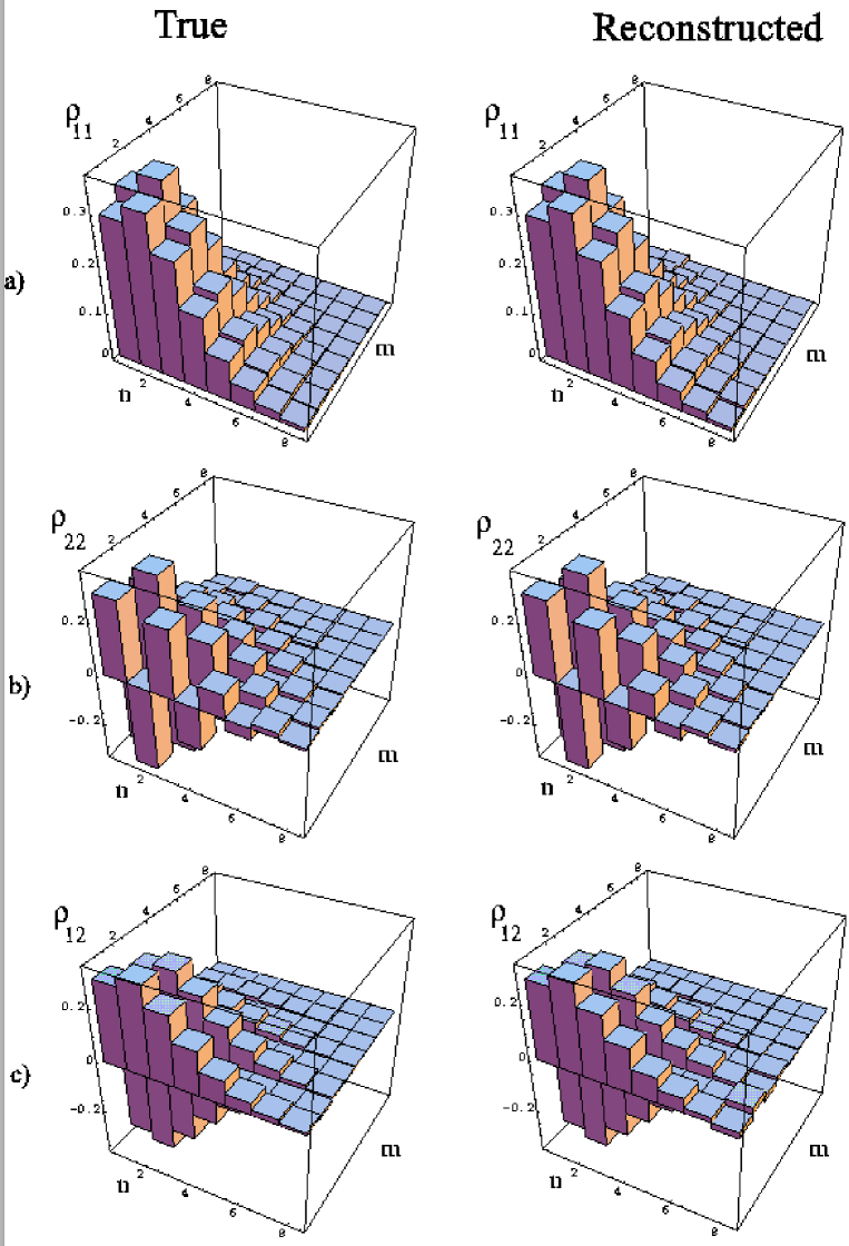
FIG. 1.: Simulated tomographic reconstruction of the density matrix for the state of Eq. (61) with $c_{1}=1/2$, $c_{2}=\sqrt{3}/2$, $\theta=\pi$, $\xi=\pi$, and $\gamma=1$. The quantum efficiency is $\eta=0.9$ and 10⁶ data per phase have been simulated. In this simulation an amplitude $|\alpha|=0.7$ of the applied reference field has been used. a) $(\rho_{11})_{n,m}$, b) $(\rho_{22})_{n,m}$, and c) $(\rho_{12})_{n,m}$. Here and in the following figures the ideal distributions are displayed on the left, whereas the reconstructed ones are displayed on the right.

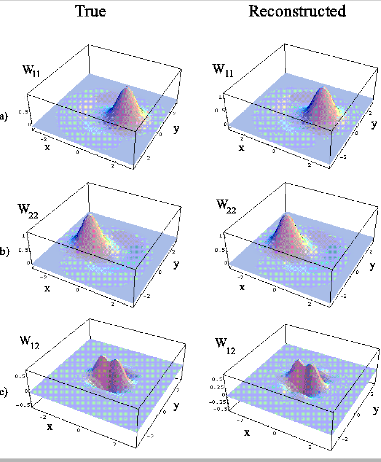
FIG. 2.: Simulated tomographic reconstruction of the Wigner functions for the state of Eq. (61) with the same parameters as in Fig. 1. a) $W_{11}(x,y)$, b) $W_{22}(x,y)$, and c) $W_{12}(x,y)$.

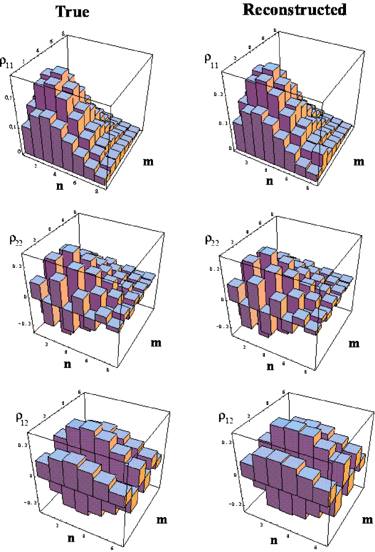
FIG. 3.: Simulated tomographic reconstruction of the density matrix for the state of Eq. (61) with $c_{1}=c_{2}=\sqrt{2}/2$, $\theta=0$, $\xi=\pi$, and $\gamma=1.5$. The quantum efficiency is $\eta=0.9$ and 10⁶ data per phase have been simulated. In this simulation an amplitude $|\alpha|=1.2$ of the applied reference field has been used. Top: $(\rho_{11})_{n,m}$; Middle: $(\rho_{22})_{n,m}$; Bottom: $(\rho_{12})_{n,m}$.

FIG. 4.: Simulated tomographic reconstruction of the Wigner functions for the state of Eq. (61) with the same parameters as in Fig. 3. Top: $W_{11}(x,y)$; Middle: $W_{22}(x,y)$; Bottom: $W_{12}(x,y)$.

- [1] L. S. Brown and G. Gabrielse, Rev. Mod. Phys. 58, 233 (1986).
- [2] S. Peil and G. Gabrielse, Phys. Rev. Lett. 83, 1287 (1999).
- [3] K. Vogel and H. Risken, Phys. Rev. A 40, R2847 (1989).
- [4] M. Freyberger, P. Bardroff, C. Leichtle, G. Schrade, and W.P. Schleich, Physics World 10 (11), 41 (1997).
- [5] D. T. Smithey, M. Beck, M. G. Raymer and A. Faridani, Phys. Rev. Lett. 70, 1244 (1993).
- [6] P. J. Bardroff, E. Mayr and W. P. Schleich, Phys. Rev. A 51, 4963 (1995).
- [7] L. G. Lutterbach and L. Davidovich, Phys. Rev. Lett. 78, 2547 (1997).
- [8] M. G. Raymer, M. Beck, and D. McAlister, Phys. Rev. Lett. 72, 1137 (1994); M. G. Raymer, D. F. McAlister, and U. Leonhardt, Phys. Rev. A 54, 2397 (1996); Th. Richter, Phys. Lett. A 211, 327 (1996); D. F. McAlister and M. G. Raymer, J. Mod. Opt. 44, 2359 (1997); M. S. Kim and G. S. Agarwal, Phys. Rev. A 59, 3044 (1999); M. G. Raymer and A. Funk, Phys. Rev. A 61, 015801 (2000). See also D.-G. Welsch, W. Vogel, and T. Opatrný in Progress in Optics, XXXIX, E. Wolf ed. (North-Holland, Amsterdam, 1999) and references therein.
- [9] E. Schrödinger, Naturwiss. 23, 807 (1935).
- [10] C.H. Bennett et al., Phys. Rev. Lett. 70, 1895 (1993).
- [11] D. Bouwmeester et al., Nature (London) 390, 575 (1997). D. Boschi et al., Phys. Rev. Lett. 80, 1121 (1998). A. Furusawa et al., Science, 282 706 (1998).
- [12] C.H. Bennett and S.J. Wiesner, Phys. Rev. Lett. 69, 2881 (1992).
- [13] M. Zukowski et al., Phys. Rev. Lett. 71, 4287 (1993). J.-W. Pan et al., Phys. Rev. Lett. 80, 3891 (1998).
- [14] A. K. Ekert, Phys. Rev. Lett. 67, 661 (1991).
- [15] See, e.g., the special issue of Proc. R. Soc. London Ser. A 454, 1969 (1998). C. H. Bennett and D. P. DiVincenzo, Nature (London) 404, 247 (2000).
- [16] C. A. Sackett et al., Nature (London) 404, 256 (2000).
- [17] S. Mancini and P. Tombesi, Phys. Rev. A 56, 3060 (1997).
- [18] W. H. Zurek, Phys. Today 44(10), 36 (1991).
- [19] S. Wallentowitz, R. L. de Matos Filho, and W. Vogel, Phys. Rev. A 56, 1205 (1997).
- [20] S. Mancini, P. Tombesi, and V. I. Man’ko, Europhys. Lett. 37, 79 (1997).
- [21] S. Mancini, M. Fortunato, P. Tombesi, and G. M. D’Ariano (submitted to J. Opt. Soc. Am. A).
- [22] G. M. D’Ariano, U. Leonhardt, and H. Paul, Phys. Rev. A 52, R1801 (1995).
- [23] M. Beck, D.T. Smithey, and M.G. Raymer, Phys. Rev. A 48, R890 (1993); D.T. Smithey, M. Beck, J. Cooper, and M.G. Raymer, ibid. 48, 3159 (1993).
- [24] G. Breitenbach, S. Schiller, and J. Mlynek, Nature (London) 387, 471 (1997).
- [25] K. Banaszek and K. Wodkiewicz, Phys. Rev. Lett. 76, 4344 (1996).
- [26] T. Opatrny and D. G. Welsh, Phys. Rev. A 55, 1462 (1997).
- [27] K. E. Cahill and R. J. Glauber, Phys. Rev. 177, 1857 (1969); ibid. 1882 (1969).
- [28] M. O. Scully and W. E. Lamb, Phys. Rev. 179, 368 (1969).
- [29] M. Hillery, R.F. O’Connell, M.O. Scully and E.P. Wigner, Phys. Rep. 106, 121 (1986).
- [30] D. Vitali, P. Tombesi, and G. J. Milburn, Phys. Rev. A 57, 4930 (1998).
- [31] S. Mancini, A. M. Martins, and P. Tombesi, Phys. Rev. A 61, 012303 (2000).