Reconstruction of SU(1,1) States [1]

Abstract

We show how group symmetries can be used to reconstruct quantum states. In our scheme for SU(1,1) states, the input field passes through a non-degenerate parametric amplifier and one measures the probability of finding the output state with a certain number (usually zero) of photons in each mode. The density matrix in the Fock basis is retrieved from the measured data by least squares method after singular value decomposition of the design matrix. Several illustrative examples involving the reconstruction of a pair coherent state, a Perelomov coherent state, and a coherent superposition of pair coherent states are considered.

PACS Nos. 42.30.Wb, 42.50Dv, 42.50Md, 42.50-p, 03.65Bz.

I Introduction

The problem of the reconstruction of quantum states was first considered in the fifties by Fano [3] and Pauli [4]. Since a quantum system is completely described by its density matrix, the task is essentially to reconstruct the density matrix of a system from information obtained by a set of measurements performed on an ensemble of identically prepared systems. To that end, the seminal work of Vogel and Risken [5] showed that for a single mode optical field, the histograms of quadrature amplitude distributions measured by homodyne detection, is just the Radon transform (or tomography) of the corresponding Wigner function. One can thus obtain the Wigner function by taking the inverse Radon transform of the data. Finally, the density matrix in the position representation is obtained from the Wigner function by Fourier transformation. This is the basis of optical homodyne tomography [5, 6, 7, 8]. The technique was experimentally realized by Smithey et al [6] who obtained the Wigner function and the density matrix of vacuum and quadrature-squeezed states of a mode of the electromagnetic field by using balanced homodyne detection. Much progress has been achieved in this field over the last few years [8]. It is now well known, for example, that one can determine the density matrix directly from the measured quadrature distribution without having to evaluate the Wigner function. Additionally, parallel tomographic schemes such as symplectic tomography [9], and photon number tomography [10] have been suggested for the reconstruction of quantum states of the light field which can even be multi-mode [11]. Other quantum systems for which reconstruction procedures were proposed include one-dimensional wave packets [12], harmonic and anharmonic molecular vibrations [13], motional states of atom beams [14], Bose-Einstein condensates [15], cyclotron states of a trapped electron [16], atomic Rydberg wave functions [17], atoms in optical lattices [18], systems with a finite-dimensional state space (e.g., for spin) [19] and states in cavity QED [20]. Experimental reconstructions were reported for electronic angular momentum states of hydrogen [21], vibrational quantum states of a diatomic molecule [22] and motional state of a single trapped atom [23]. Vasilyev et al [24] have reported tomographic measurement of joint photon statistics of the two-mode quantum state produced in parametric amplification.

While extensive work has been done on states of a two-mode field, there are very many physical situations where the state to be reconstructed has certain group symmetry. Clearly one could benefit considerably by the use of the group symmetry properties in the reconstruction of the state. For example, in the process of down conversion, the two photons are produced together. In this case the difference in the photon number in the two modes is conserved and the state has the symmetry property of the SU(1,1) group. In a previous publication, one of us has discussed how the underlying SU(2) symmetry of a state can be utilized very efficiently for its reconstruction [25]. In this paper, we consider reconstruction of states whose symmetry group is SU(1,1) [26]. The plan of the paper is as follows. In section 2, we present a group theoretic perspective of a general reconstruction procedure for quantum states. In section 3, we apply our method to reconstruct some important SU(1,1) states. The paper ends with concluding remarks in section 4.

II Using Group Symmetries for State Reconstruction

Let us first recall the principles of photon number tomography. Several workers have suggested a procedure whereby the initial state of the radiation field described by the density matrix $\rho^{(in)}$, is displaced by different amounts.

$$\rho^{(in)}\rightarrow\rho^{(out)} = {\cal D}^{\dagger}(\alpha)\rho^{(in)}{\cal D}(\alpha),$$ (1)

$${\cal D}(\alpha) = \exp(\alpha a^{\dagger}-\alpha^{*}a),$$ (2)

One then measures the distribution of photons in the displaced field. The photon count in the output field is used to reconstruct the $s$-ordered distribution function of the input field. This method was very successfully used to measure the vibrational state of a trapped ion [23]. There is a related suggestion in the context of cavity QED which yields the characteristic function of the radiation field [20]. In both these situations one measures atomic populations with rather high efficiency. Though a direct photon counting measurement suffers from questions of poor efficiency of photodetectors, there exist several proposals on how to go around the problem [27].

For the two-mode field with SU(2) symmetry, one can displace the state using the corresponding unitary operator for the SU(2) group. This has been shown to enable one to reconstruct the states of spin systems, states of polarization etc [25]. This is also closely related to a proposal in the context of Bose Einstein condensates [15]. The displacement of the state is physically realized (say) by using external fields in the case of two-level atoms or spins. In the case of radiation fields such a displacement is realized by optical components like waveplates [28].

We next consider the case when the underlying symmetry of the state is of the SU(1,1) group. The generators of this group are

$$K_{+}=a^{\dagger}b^{\dagger},\quad K_{-}=ab,\quad K_{z}=(a^{\dagger}a+b^{\dagger}b+1)/2,$$ (3)

where $a^{\dagger}a-b^{\dagger}b$ = constant = $q$ (say). Without any loss of generality, one can assume that $q\geq 0$. In that case, the vacuum state is given by the two-mode Fock state $|q,0\rangle$ with the property $K_{-}|q,0\rangle=0$. The displacement operator for this group is the well known squeezing operator parametrized by a complex quantity $z$:

$${\cal S}(z)=\exp(za^{\dagger}b^{\dagger}-z^{*}ab).$$ (4)

Acting on the $|0,0\rangle$ state, it produces the squeezed vacuum state

$$|z\rangle_{0}={\cal S}(z)|0,0\rangle.$$ (5)

It should be noted that even though we are dealing with the two-mode field, the underlying symmetry makes ${\cal S}(z)$ different from the product ${\cal D}(\alpha){\cal D}(\beta)$ of the displacement operators. We can now proceed in the spirit of earlier constructions for the Heisenberg-Weyl and the SU(2) groups. We consider the operator defined by

$$\rho^{(out)}={\cal S}^{\dagger}(z)\rho^{(in)}{\cal S}(z).$$ (6)

and the measurement of (say) $q$ photons in mode $a$ and no photons in mode $b$, i.e., the quantity

$$p^{(out)}(q,0) = \langle q,0|\rho^{(out)}|q,0\rangle$$ (7)

$$= \langle q,0|{\cal S}^{\dagger}(z)\rho^{(in)}{\cal S}(z)|q,0\rangle$$ (8)

$$= {}_{q}\langle z|\rho^{(in)}|z\rangle_{q}\equiv{\cal Q}(q,z)$$ (9)

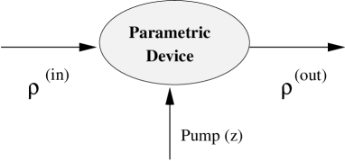
where $|z\rangle_{q}$ is defined in analogy to Eq (5) with $|0,0\rangle$ replaced by $|q,0\rangle$. We would now like to demonstrate how measurements of ${\cal Q}(q,z)$ for a range of values of $z$ can be used to reconstruct the input state $\rho^{(in)}$. In this case, as indicated in Fig. 1, $\rho^{(out)}$ can be obtained from $\rho^{(in)}$ by passing the input state through a nondegenerate parametric amplifier whose action is described by the Hamiltonian $H=\lambda a^{\dagger}b^{\dagger}+h.c$ where $\lambda$ is related to the non-linear susceptibility. The operator ${\cal S}(z)$ is simply the evolution operator for this Hamiltonian with $z=i\lambda t$.

FIG. 1.: Schematic of the reconstruction procedure.

Using the disentangling theorem for ${\cal S}$ and substituting in the expression for ${\cal Q}(q,z)$, we can write this probability as a function of two auxiliary, experimentally controlled parameters

$$y=\tanh^{2}|z|,\quad\phi=i\ln\left({z\over|z|}\right).$$ (10)

After some algebra, one obtains

$${\cal Q}(q,z)\equiv{\cal Q}(q,y,\phi)={(1-y)^{q+1}\over q!}\times$$ (12)

$$\sum_{m,n=0}^{\infty}\sqrt{{(m+q)!(n+q)!\over m!n!}}e^{i(m-n)\phi}y^{(m+n)/2}\rho_{n,m}(q).$$

For the sake of clarity, we have used the notation $\langle n+q,n|\rho^{(\rm in)}|m+q,m\rangle=\rho_{n,m}(q)$. At this point, we make the physically reasonable assumption that

$$\rho_{n,m}(q)\approx 0,\quad\hbox{for}\quad m,n>n_{\rm max},$$ (13)

if $n_{\rm max}$ is suitably large [30]. Next we introduce the Fourier Transform of the probability data with respect to the phase angle $\phi$:

$$g_{k}(q,y)=\int_{0}^{2\pi}{d\phi\over 2\pi}e^{ik\phi}{\cal Q}(q,y,\phi),$$ (14)

and construct the quantity

$$f_{k}(q,y)={g_{k}(q,y)y^{-k/2}\over(1-y)^{q+1}}.$$ (15)

The construction is legitimate since the potentially singular points $y=0$ and $y=1$ are inaccessible to the experimenter. The point $y=0$ corresponds to ‘doing nothing’ to the input state whereas $y=1$ would correspond to $|z|$ (and hence, either the pump amplitude or the duration of the experiment) being infinity.

The integration over $\phi$ yields a Kronecker delta function and one obtains a simple power series expansion for $f_{k}(q,y)$:

$$f_{k}(q,y)=\sum_{m=0}^{n_{\rm max}-k}B_{mk}(q)\rho_{m+k,m}(q)y^{m},$$ (16)

where

$$B_{mk}(q)={1\over q!}\sqrt{{(m+k+q)!(m+q)!\over m!(m+k)!}}.$$ (17)

The task now is to obtain the density matrix elements from tabulated values of $f_{k}(q,y)$. This can be done, in principle, by least squares inversion [30].

1 Least Squares Method

We write $f_{k}(q,y)$ in the form $f_{k}(q,y)=\sum_{j=1}^{M}a_{j}^{(M)}\phi_{j}(y)$ where $\phi_{j}(y)=y^{j-1}$ are the basis functions, $a_{j}^{(M)}=B_{j-1,k}(q)\rho_{j-1+k,j-1}(q)$ contain the unknown density matrix elements, and $M=n_{\rm max}-k+1$. Here the superscript $(M)$ denotes that the coefficients in general, depend on the number of basis functions included in the approximation. Let $\tilde{y}_{1}$, $\tilde{y}_{2}$,…,$\tilde{y}_{N}$ be a set of points at which the values of $f_{k}(q,y)$ are measured. We denote by $\tilde{f}_{i}$ the measured value at $\tilde{y}_{i}$ with an error $\tilde{f}_{i}-f_{k}(q,\tilde{y}_{i})$. It is generally assumed that the error at different points is uncorrelated. The design matrix $G$ is an $N\times M$ matrix whose $ij$-th element is given by $G_{ij}=\phi_{j}(\tilde{y}_{i})$. We introduce two vectors $\vec{a}=\{a_{1},a_{2},....a_{M}\}$ and $\vec{b}=\{\tilde{f}_{1},\tilde{f}_{2},.....\tilde{f}_{N}\}$. In least squares method, the coefficients $a_{j}$ are determined by minimizing the quantity $\chi^{2}=|G\vec{a}-\vec{b}|^{2}$.

Although the method of least squares finds extensive use in literature, it will give meaningful values for the coefficients $\rho_{m+k,m}(q)$ only for small values of $m$. This is so because for large values of $m$, the corresponding normal equations become ill-conditioned. Hence we cannot expect to solve them unless very high precision arithmetic is used. Even then a slight change in the data (due for example, to round-off error) may change the solution significantly. This ill-conditioning can be traced to the fact that for large values of $m$, the basis functions $y^{m}$ are not really independent in the sense that there will be little difference between terms of (say) $y^{9}$ and $y^{10}$ if the precision in the measured data is unable to resolve it. In such cases, one must use Tikhonov regularization or Singular Value Decomposition (SVD) of the design matrix in order to extract meaningful results for the unknown coefficients $\rho_{m+k,m}(q)$. We adopt the SVD approach [31] in which one works directly with the design matrix $G$ rather than with $G^{T}G$ (as in the least squares method without SVD). Thus the ill-conditioning gets much reduced. The design matrix $G$ is written in the form $G=U\Sigma V^{T}$, where $U$ is a $N\times M$ matrix, $\Sigma$ is a $M\times M$ diagonal matrix with diagonal elements $\sigma_{1}$, $\sigma_{2}$, …. $\sigma_{M}$, and $V$ is a $M\times M$ orthogonal matrix so that $U^{T}U=V^{T}V=VV^{T}=I_{M}$, the $M\times M$ unit matrix. The matrix $U$ consists of $M$ orthonormalised eigenvectors associated with the $M$ largest eigenvalues of $GG^{T}$, and the matrix $V$ consists of the orthonormalised eigenvectors of $G^{T}G$. The diagonal elements of $\Sigma$ are the nonnegative square roots of the eigenvalues of $G^{T}G$ and are called the singular values. If $\vec{u_{i}}$ and $\vec{v_{i}}$ are the $i$-th columns of $U$ and $V$ respectively, then the solution can be written as $\vec{a}=\sum_{i=1}^{M}\left(\vec{u_{i}}\cdot\vec{b}/\sigma_{i}\right)\vec{v_{i}}$. The variance in the estimated parameters $a_{j}$ can be written as $\sigma^{2}(a_{j}^{(M)})=\sum_{i=1}^{M}v^{2}_{ji}/\sigma^{2}_{i}$. It can thus be seen that the error will be rather large for small $\sigma_{i}$, and dropping such terms will reduce the errors, at the cost of increasing the mean square deviation slightly. The columns of $V$ corresponding to small $\sigma_{i}$ identify the linear combination of variables, which contribute little towards reducing $\chi^{2}$, but make large contribution in the standard deviation. Thus even if some of the singular values are not small enough to cause round-off problems, it may be better to zero them while computing the solution.

III Results and Discussion

In this section we will reconstruct the density matrix from a simulation of the corresponding probability data for a pair coherent state [32], a Perelomov [29] coherent state and a coherent superposition of pair coherent states.

In a real experiment the parameters $y$ and $\phi$ can take only a finite (however large) number of values. In the absence of any a priori knowledge about the input state, we choose a set of values of $\phi$ equally distributed between $0$ and $2\pi$: $\phi_{s}=2\pi s/N_{\phi}$, and a set of values of $y$ which are equi-spaced between $y_{\rm min}=0.1$ and $y_{\rm max}=0.9$: $\tilde{y}_{n}=y_{\rm min}+(y_{\rm max}-y_{\rm min})(n-1)/(N-1)$. Then the Fourier transform with respect to $\phi$ in Eq. (14) is approximated by a discrete Fourier transform

$$g_{k}(q,\tilde{y}_{i})\rightarrow{1\over N_{\phi}}\sum_{s=0}^{N_{\phi}-1}e^{2\pi iks/N_{\phi}}{\cal Q}(q,\tilde{y}_{i},2\pi s/N_{\phi}).$$ (18)

Thus apart from truncation error due to the assumption (13), one will also have to deal with error due to discretization of the variables $y$ and $\phi$. The systematic error due to phase discretization can be reduced to zero by choosing $N_{\phi}\geq 2n_{\rm max}+1$ [30] whereas the error in the discretization of $y$ is of order $N^{-2}$ and can be made arbitrarily small by taking a sufficiently large value of $N$. We have set $N_{\phi}=20$ and $N=101$ in the calculations to follow. The data was simulated in the following way. We add to the exact probability data $f_{k}(q,\tilde{y}_{i})$ an error term $\delta f_{k}(q,\tilde{y}_{i})=R{\cal G}(f_{k}(q,\tilde{y}_{i}))\sqrt{f_{k}(q,\tilde{y}_{i})/\tau}$, where $R$ is a real random number uniformly distributed between -1 and 1, ${\cal G}$ is a Gaussian distribution with zero mean and unit variance [33], and $\tau=20000$ is the number of trials at $y=\tilde{y}_{i}$. All our calculations have been carried out using the software package Mathematica. For the record, the random numbers were generated with a seed value of 45.

A Reconstruction of a pair coherent state

Pair coherent states of the radiation field can be generated via the competition of four-wave mixing and two-photon absorption in a nonlinear medium [32]. Pair coherent states can also be realized for the motion of a trapped ion [34]. One drives the ion with a laser on resonance and two other lasers with appropriately chosen directions of propagation and tuned to the second lower vibrational side band. In the Lamb-Dicke limit, the ion is found in a pair coherent state.

The state vector for a pair coherent state has the form

$$|\Phi(\xi,p)\rangle = N(\xi,p)\sum_{n=0}^{\infty}{{\xi}^{n}\over\sqrt{n!(n+p)!}}|n+p,n\rangle,$$ (19)

$$N(\xi,p) = \left[\sum_{n=0}^{\infty}{|{\xi}|^{2n}\over n!(n+p)!}\right]^{-1/2}.$$ (20)

Here $\xi$ is a complex parameter and $p\geq 0$ is an integer. The corresponding exact density matrix elements in the Fock basis are given by

$$\rho_{n,m}(p)=|N_{p}|^{2}{{\xi}^{n}{{\xi}^{*}}^{m}\over\sqrt{n!(n+p)!m!(m+p)!}}$$ (21)

Note that $\rho_{m,n}(p)=\rho_{n,m}^{*}(p)$ and for real values of $\xi$, the density matrix is symmetric.

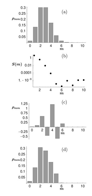
The exact diagonal density matrix elements for the state $|\Phi(3,0)\rangle$ are plotted in Fig. 2(a). The least squares reconstruction from the simulated data fails in this case (some of the diagonal elements assume absolute values of the order of $10^{3}$ or so!) even with SVD when the tolerance parameter is set to its default value of $10^{-p+2}$ where $p$ is the machine precision. The failure is due to overfitting, that is, the use of a higher degree polynomial for $f_{0}(0,\tilde{y}_{i})$ than necessary. As a result, the design matrix becomes ill-conditioned and some of the diagonal elements of $\Sigma$ become very small. We mention parenthetically that the default tolerance removes none of these singular (or almost singular) values.

The situation can be improved substantially by probing certain diagnostic indicators. The sequential sum of squares, for example, is useful in determining the degree of the univariate polynomial model. Each element in the sequential sum of squares vector corresponds to the increment in the model sum of squares obtained by sequentially adding each (non-constant) basis function to the model. It can be seen from Fig. 2(b) that the contribution of the basis functions $y^{m}$ in this respect decreases rapidly and monotonically up to $m=6$ and is negligible (albeit oscillatory) thereafter, suggesting that the optimum degree of the polynomial for $f_{0}(q,\tilde{y}_{i})$ should be five or six.

FIG. 2.: Reconstruction of the diagonal density matrix elements $\rho_{mm}$ of the pair coherent state $|\Phi(3,0)\rangle$ (see Eqs. (15) and (16)) by least squares method. (a) Exact values; (b) sequential sum of squares $S(m)$ as a function of the order $m$ of the fitting polynomial suggests that the optimum degree of the polynomial should be five or six; (c) reconstruction by using a sixth degree fitting polynomial for $f_{0}(0,\tilde{y}_{i})$; (d) as in (c), but with the singular values $<0.1$ removed.

Furthermore, if the errors are uncorrelated, then the residuals $r_{i}=\tilde{f}_{i}-\sum_{j=1}^{M}a_{j}^{(M)}\phi_{j}(\tilde{y}_{i})$ should be randomly distributed and if we count the number of sign changes $S_{c}$ in the sequence $r_{1}$, $r_{2}$, ….$r_{N}$, then we should find a value close to $N/2$ (that is, within about $\sqrt{N/2}$). Thus, after adding every term, we can check the number of sign changes and decide to terminate the process when this number increases to its limiting value. In the fitting of $f_{0}(0,\tilde{y}_{i})$, the values of $S_{c}$ are found to be 3, 36, 49, 49, 49, 54, 51, 52 and 55 when the degree of the fitted polynomial is increased from 2 to 10 in steps of unity. With 101 data points, it can be seen that $S_{c}$ reaches its terminal value when the degree of the polynomial is $\geq 4$.

Based on these observations, we fit $f_{0}(0,\tilde{y}_{i})$ by a 6-th degree polynomial instead of the 10th degree polynomial originally implied in Eq. (12). This does not mean that $n_{\rm max}$ is re-set to six. It simply means that reliable estimates cannot be made for $\rho_{m,m}$ if $m$ is greater than six. The reconstructed diagonal density matrix elements as plotted in Fig. 2(c) are still not quite in agreement with the exact results but are at least of the same order of magnitude. The diagonal elements of the $7\times 7$ matrix $\Sigma$ have the values $12.2716$, $4.00265$, $0.964488$, $0.176915$, $0.0245331$, $0.00247435$, $0.00015933$. Setting the smallest three elements and their inverses to zero, one obtains a more realistic reconstruction of the diagonal density matrix elements (Fig. 2(d)).

FIG. 3.: Reconstruction of the density matrix elements $\rho_{mn}$ of the pair coherent state $|\Phi(3,0)\rangle$ by least squares method after singular value decomposition of the design matrix. The truncation parameter was set at $n_{\rm max}=10$. (a) Exact values; (b) reconstructed values; (c) the difference between the exact and the reconstructed values.

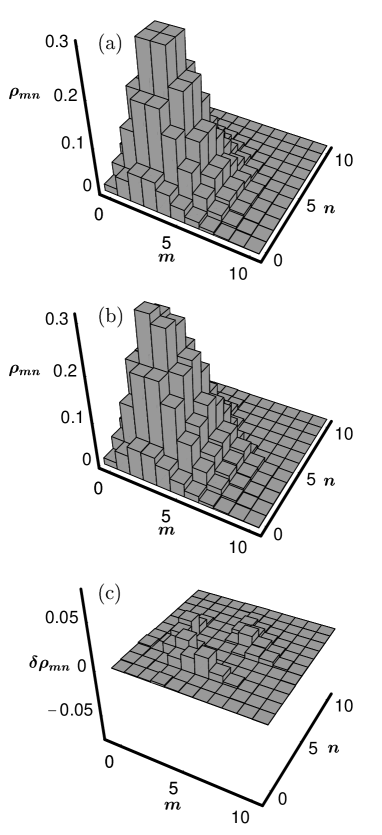
We note that overfitting occurs only for values of $k$ close to zero and is worst for the diagonal elements. A systematic and consistent repetition of the above exercise for other values of $k$ reveals that the optimum degree of the polynomial is $5$ for $k=1$ and $2$, $4$ for $3\leq k\leq 5$ and is $n_{\rm max}-k$ for $6\leq k\leq n_{\rm max}$. Removing the singular values $<0.1$ in each case, we can finally reconstruct all the elements of the density matrix. The result is in reasonable agreement with the exact density matrix elements as seen in Fig. 3.

B Reconstruction of a Perelomov coherent state

It is well known that Perelomov coherent states can be produced in parametric interactions. The state vector for a Perelomov coherent state is given by

$$|\Psi(\eta,q)\rangle={(1-|\eta|^{2})^{{q+1\over 2}}\over\sqrt{q!}}\sum_{p=0}^{\infty}\eta^{p}\sqrt{{(p+q)!\over p!}}|p+q,p\rangle,$$ (22)

where $\eta$ is, in general, a complex parameter with $|\eta|<1$, and $q\geq 0$ is an integer. The corresponding exact density matrix elements in the Fock basis have the expression

$$\rho_{n,m}(q)={(1-|\eta|^{2})^{q+1}\over q!}\sqrt{{(n+q)!(m+q)!\over n!m!}}\eta^{n}{\eta^{*}}^{m}.$$ (23)

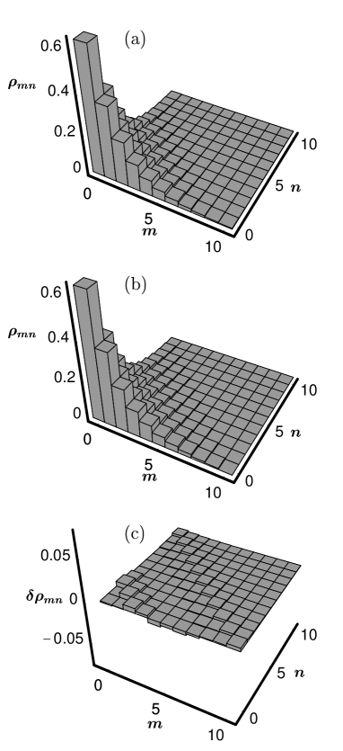
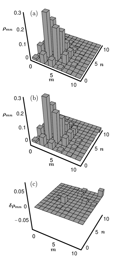
For $q=0$ and real values of $\eta$, the density matrix is not only symmetric but also has the following additional symmetries: $\rho_{n+2k,n}(0)=\rho_{n+k,n+k}(0)$ and $\rho_{n+2k+1,n}(0)=\rho_{n+k+1,n+k}(0)$. Consequently, only $f_{0}(0,y)$ and $f_{1}(0,y)$ need to be measured and modeled. We choose $q=0$, $\eta=0.6$ and set $n_{\rm max}=10$. Proceeding as before, we plot the exact density matrix elements in Fig. 4 along with the computed elements reconstructed by the least squares method with singular value decomposition. Once again, the reconstruction is found to be satisfactory. The error in the computed elements is seen to be slightly less than in the case of pair coherent states as only 4th order fitting polynomials were necessary in the present case. Using the method of optical homodyne tomography, Vasilyev et al [24] have, for the first time, reconstructed the diagonal elements of the two-mode Perelomov coherent state produced by a parametric amplifier. Their experiment also demonstrates how well the SU(1,1) symmetry holds in parametric amplification.

FIG. 4.: Same as in figure 3 but for a Perelomov coherent state $\Psi(0.5,0)$ (see Eqs. (17) and (18)).

C Reconstruction of a coherent superposition of pair coherent states

Our final example is the reconstruction of a coherent superposition of pair coherent states $|\Phi(\pm 3,0)\rangle$:

$$|\psi\rangle={e^{-i\pi/4}\over\sqrt{2}}\left[|\Phi(3,0)\rangle+|\Phi(-3,0)\rangle\right].$$ (24)

It can be easily shown that the $nm$-th density matrix element of $|\psi\rangle$ will be non-zero only when both $n$ and $m$ are even in which case its value will equal the $nm$-th density matrix element of $|\Phi(\pm 3,0)\rangle$. As a result, only even values of $k$ and even powers of $y$ appear in the modeling of $f_{k}(0,y)$. As shown in Fig. 5, satisfactory agreement is obtained between the exact and reconstructed density matrix elements.

FIG. 5.: Same as in figure 3 but for a coherent superposition of pair coherent states $|\Phi(\pm 3,0)\rangle$ (see Eq. (19)).

IV Conclusion

We have suggested a simple scheme for the reconstruction of two-mode SU(1,1) states using parametric amplifiers. The probability of the output state being in a certain two-mode number state is measured. The probability data is then ‘inverted’ to extract the density matrix of the input state by taking advantage of certain symmetries in the input state. We have shown that this inversion can be achieved by the least squares method after singular value decomposition of the design matrix.

REFERENCES

- [1] A preliminary account of this work was presented by G. S. Agarwal at the Sixth International Conference on Squeezed States and Uncertainty Relations (ICSSUR VI), Napoli, Italy, May24-29, 1999.
- [2] Also at Jawaharlal Nehru Centre for Advanced Scientific Research, Bangalore, India
- [3] U. Fano, Rev. Mod. Phys. 29, 74 (1957).
- [4] W. Pauli, in Encyclopedia of Physics (Springer, Berlin, 1958), Vol. 5, p. 17.
- [5] K. Vogel and H. Risken, Phys. Rev. A 40, 2847 (1989)
- [6] D. T. Smithey, M. Beck, M. G. Raymer, and A. Faridani, Phys. Rev. Lett. 70, 1244 (1993); D. T. Smithey, M. Beck, J. Cooper, M. G. Raymer, and A. Faridani, Phys. Scr. T48, 35 (1993); M. Munroe, D. Boggavarapu, M. E. Anderson, and M. G. Raymer, Phys. Rev. A 52, R924 (1995)
- [7] G. M. D’Ariano, C. Macchiavello, and M. G. A. Paris, Phys. Lett. A 195, 31 (1994); Phys. Rev. A 50, 4298 (1994); H. Kühn, D. -G. Welsch, and W. Vogel, J. Mod. Opt. 41, 1607 (1994); A. Wünsche, ibid. 44, 2293 (1997); U. Leonhardt, M. Munroe, T. Kiss, Th. Richter, and M. G. Raymer, Opt. Commun. 127, 144 (1996); U. Leonhardt, H. Paul, and G. M. D’Ariano, Phys. Rev. A 52, 4899 (1995); U. Leonhardt, and M. Munroe, ibid. 54, 3682 (1996).
- [8] For a survey, see U. Leonhardt, Measuring the Quantum State of Light (Cambridge Univ. Press, Cambridge, 1997); D. -G. Welsch, W. Vogel, and T. Opatrný, in Progress in Optics, Ed. E. Wolf, (North Holland, Amsterdam), 39, 63 (1999).
- [9] D. F. V. James and G. S. Agarwal, J. Opt. Soc. Am. B 12, 704 (1995); S. Mancini, V. I. Man’ko, and P. Tombesi, Quantum Semiclass. Opt. 7, 615 (1995); G. M. D’Ariano, S. Mancini, V. I. Man’ko, and P. Tombesi, ibid. 8, 1017 (1996); V. I. Man’ko, J. Russ. Laser Research 17, 579 (1996).
- [10] K. Banaszek and K. Wódkiewicz, Phys. Rev. Lett. 76, 4344 (1996); S. Wallentowitz and W. Vogel, Phys. Rev. A 53, 4528 (1996); T. Opatrný and D. -G. Welsch, ibid. 55, 1462 (1997); T. Opatrný, D. -G. Welsch, S. Wallentowitz, and W. Vogel, J. Mod. Opt., 44, 2405 (1997); S. Mancini, P. Tombesi, and V. I. Man’ko, Europhys. Lett. 37, 79 (1997).
- [11] G. S. Agarwal and S. Chaturvedi, Phys. Rev. A 49, R665 (1994); G. M. D’Ariano, M. Vasilyev, and P. Kumar, ibid. 58, 636 (1998); H. Kühn, D. -G. Welsch, and W. Vogel, ibid. 51, 4240 (1995); M. G. Raymer, D. F. McAlister, and U. Leonhardt, ibid.54, 2397 (1996); T. Opatrný, D. -G. Welsch and W. Vogel, Opt. Commun. 134, 112 (1997); Th. Richter, J. Mod. Opt. 44, 2385 (1997); Phys. Rev. A 55, 4629 (1997); H. Paul, P. Torma, T. Kiss, and I. Jex, J. Mod. Opt. 44, 2395 (1997).
- [12] A. Royer, Phys. Rev. Lett. 55, 2745 (1985); Found. Phys. 19, 3 (1989); U. Leonhardt and M. G. Raymer, Phys. Rev. Lett. 76, 1985 (1996); D. S. Kraehmer and U. Leonhardt, Appl. Phys. B 65, 725 (1997); U. Leonhardt and S. Schneider, Phys. Rev. A 56, 2549 (1997); M. G. Raymer J. Mod. Opt. 44, 2565 (1997).
- [13] U. Leonhardt, Phys. Rev. A 55, 3164 (1997); T. Opatrný, D. -G. Welsch, and W. Vogel, ibid. 56, 1788 (1997); L. Davidovich, M. Orszag, and N. Zagury,ibid. 57, 2544 (1998).
- [14] U. Janicke and M. Wilkens, J. Mod. Opt. 42, 2183 (1995); T. Pfau and Ch. Kurtsiefer, ibid. 44, 2551 (1997); D. A. Kokorowski and D. E. Pritchard, ibid. 44, 2575 (1997); Ch. Kurtsiefer, T. Pfau, and J. Mlynek, Nature (London) 386, 150 (1997); S. H. Kienle, D. Fischer, W. P. Schleich, V. P. Yakovlev, and M. Freyberger, Appl. Phys. B 65, 735 (1997).
- [15] S. Mancini and P. Tombesi, Europhys. Lett. 40, 351 (1997); E. L. Bolda, S. M. Tan, and D. F. Walls, Phys. Rev. Lett. 79, 4719 (1997); Phys. Rev. A 57, 4686 (1998).
- [16] S. Mancini and P. Tombesi, Phys. Rev. A 56, 3060 (1997).
- [17] X. Chen and J. A. Yeazell, Phys. Rev. A 56, 2316 (1997).
- [18] A. Zucchetti, S. Wallentowitz, W. Vogel and N. P. Bigelow, Phys. Rev. A 61, 011405 (2000).
- [19] U. Leonhardt, Phys. Rev. Lett. 74, 4101 (1995); Phys. Rev. A 53, 2998 (1996); W. Band and J. L. Park, Found. Phys. 1, 133 (1970); 1, 211 (1971);1, 339 (1971); Am. J. Phys. 47, 188 (1979); I. D. I. D. Ivanović, J. Math. Phys. 24, 1199 (1983); W. K. Wootters, Found. Phys. 16, 391 (1986); W. K. Wootters and B. D. Fields, Ann. Phys. (N. Y. ) 191, 363 (1989); V. V. Dodonov and V. I. Man’ko, Phys. Lett. A 229, 335 (1997); G. S. Agarwal, Phys. Rev. A 57, 671 (1998); M. G. Benedict and A Czirjak, ibid. 60, 4034 (1999); S. M. Chumakov, A. B. Klimov and K. B. Wolf, ibid. 61, 034101 (2000).
- [20] M. S. Kim and G. S. Agarwal, Phys. Rev. A 59, 3044 (1999); M. S. Kim, G. Antesberger, C. T. Bodendorf, and H. Walther, ibid. 58, R65 (1998); L. G. Lutterbach and L. Davidovich, Phys. Rev. Lett. 78, 2547 (1997).
- [21] J. R. Ashburn, R. A. Cline, P. J. M. van der Burgt, W. B. Westerveldt, and J. S. Risley, Phys. Rev. A 41, 2407 (1990).
- [22] T. J. Dunn, J. N. Sweetser, I. A. Walmsley, and C. Radzewicz, Phys. Rev. Lett. 70, 3388 (1993); T. J. Dunn, I. A. Walmsley, and S. Mukamel, ibid. 74, 884 (1995).
- [23] D. Leibfried, D. M. Meekhof, B. E. King, C. Monroe, W. M. Itano, and D. J. Wineland, Phys. Rev. Lett. 77, 4281 (1996).
- [24] M. Vasilyev, S. K. Choi, P. Kumar and G. M. D’Ariano, Phys. Rev. Lett. 84, 2354 (2000).
- [25] G. S. Agarwal, Phys. Rev. A 57, 671 (1998); C. Brif and A. Mann, quant-ph/9904054, (1999)
- [26] J. Banerji and G. S. Agarwal, Phys. Rev. A 59, 4777 (1999).
- [27] See for example, G. M. D’Ariano, U. Leonhardt, and H. Paul, Phys. Rev. A 52, R1801 (1995); and Welsch et al in Ref. [8].
- [28] L. Mandel and E. Wolf, Optical Coherence and Quantum Optics (Cambridge University Press, 1995) Chap. VI.
- [29] A. M. Perelomov, Generalized Coherent States and Their Applications (Springer, Berlin 1986), C. M. Caves and B. L. Shumaker, Phys. Rev. A 31, 3068, 3093 (1985).
- [30] T. Opatrný, D. -G. Welsch and W. Vogel, Phys. Rev. A 56, 1788 (1997).
- [31] See for example, H. M. Antia, Numerical Methods for Scientists and Engineers (Tata McGraw-Hill, New Delhi, 1991).
- [32] G. S. Agarwal, J. Opt. Soc. Am. B 5, 1940 (1988).
- [33] See for example, Bolda et al in Ref. [15].
- [34] S. -C. Gau, J. Steinbach, and P. L. Knight, Phys. Rev. A 54, 1014 (1996).