Experimental test of non-local quantum correlation in relativistic configurations

Abstract

We report on a new kind of experimental investigations of the tension between quantum nonlocally and relativity. Entangled photons are sent via an optical fiber network to two villages near Geneva, separated by more than 10 km where they are analyzed by interferometers. The photon pair source is set as precisely as possible in the center so that the two photons arrive at the detectors within a time interval of less than 5 ps (corresponding to a path length difference of less than 1 mm ). One detector is set in motion so that both detectors, each in its own inertial reference frame, are first to do the measurement! The data always reproduces the quantum correlations, making it thus more difficult to consider the projection postulate as a compact description of real collapses of the wave-function.

1 Introduction

Since the famous article by Einstein, Podolsky and Rosen (EPR) in 1935 [1] ”quantum non-locality”, received quite a lot of attention. They described a situation where two entangled quantum systems are measured at a distance. The correlation between the data can’t be explained by local variables, as demonstrated by Bell in 1964 [2], although they can’t be used to communicate information faster than light. Indeed, the data on both sides, although highly correlated, is random. There is thus no obvious conflict with special relativity. In a realist’s view the correlation could be ”explained” by an action of the first measurement on the second one. This explanation is intuitive, but, if the distance between the two detection events is space-like, incompatible with relativity.

This tension between quantum mechanics and relativity has long been studied by theorists, see among many others [3, 4, 5, 6, 7]. But it clearly deserves to be analyzed experimentally and the first realization of a new kind of test is the main result of this article. Let us recall that the tension is between the collapse of the quantum state (also called ”objectification” [8], or ”actualization of potential properties” [9, 10, 11]) and Lorentz invariance: since the collapse instantaneously affects the state of systems composed of distance parts, it can’t be described in a covariant way. From this observation one may conclude either that there is no collapse or that this tension indicates a place to look for new physics. The assumption that there is no real collapse sounds strange to us, though, admittedly, it deserves to be developed [12]. Anyway, in this article we follow the intuition that the tension between quantum mechanics and relativity is a guide for new physics. In order to test this tension, we design an experiment in which both quantum nonlocality and relativity play a crucial role. By quantum nonlocality we mean here measurements on two systems that are spatially separated, but still described as one global quantum object characterized by one state vector (i.e. the two systems are entangled). For relativity we like a role more prominent than mere spatial separation, as in tests of Bell inequalities. Central to relativity (at least to special relativity) is the relativity of time, which may differ between inertial frames with relative velocities. Hence, we like to have the observers of the two quantum systems not only space-like separated, but moreover in relative motion such that the chronology of the measurement events is relative to the observer: each observer in his own inertial frame performs his measurement before the other observer. In such a situation the concept of ”collapse” is even weirder: both observers equivalently claim to trigger the collapse first! Actually one can then argue, following Suarez and Scarani [13], that in such a situation each measurement is independent from the other and that the outcomes are uncorrelated (more precisely, that only classical correlation remain, the quantum correlation carried by the wave-function being broken, see appendix A).

Let us elaborate on the intuition that motivates our experiment. Each reference frame determines a time ordering. Hence, in each reference frame one measurement takes place before the other and can be considered as the trigger (the cause) of the collapse. The picture is then the following: the first measurement produces a random outcome with probabilities determined by the local quantum state (the entire state is not needed to compute the probabilities, the local state obtained by tracing over the distant system suffices). When the outcome is produced, the global quantum state is reduced. This is the controversial part of the process since this reduction happens instantaneously in theory and faster than light according to experimental tests of Bell inequality. The second measurement can then be described like the first one: it produces a random outcome with probabilities determined by the local state. The only difference with respect to the first measurement is that the local state of the second measurement contains ”information” about the outcome of the first measurement. Since this ”information” can not be used to transmit a classical message, there is no direct conflict with relativity and we term this ”information” as quantum information. Since in our experiment the time intervall between the two meaurements is minimized, it will supply a lower limit of the speed of this quantum information. So far the described picture of the collapse is compatible with relativity, and with all experiments performed so far. But let us now assume that the two observers are in relative motion such that they disagree on the time ordering of the measurements. Then, it is plausible that each measurement produces random outcomes with probabilities determined by the local sates (see appendix A):

$$Prob(++|before-before) = <P_{\alpha}\otimes\leavevmode\hbox{\small 1\kern-3.8pt\normalsize 1}>_{\psi}<\leavevmode\hbox{\small 1\kern-3.8pt\normalsize 1}\otimes P_{\beta}>_{\psi}$$ (1)

$$= Tr(P_{\alpha}\rho_{1})Tr(P_{\beta}\rho_{2})$$ (2)

where $\rho_{1}=Tr_{2}(\psi\psi^{\dagger})$ and $\rho_{2}=Tr_{1}(\psi\psi^{\dagger})$ are the local states obtained by tracing over the other sub-system and $P_{\alpha}$ and $P_{\beta}$ the projectors corresponding to the two measurements. For singlet states, for example, the probability of (++) outcomes would be $\frac{1}{4}$, independently of the orientations of the analyzers. The above prediction, based on plausible intuition inspired by the work of Suarez and Scarani [13], differs from the quantum predictions. However, it does not contradict any experimental result and deserves thus to be tested experimentally.

At first sight the experiment may seem exceedingly difficult. First, because it requires relativistic speeds in order to have different time ordering. Next, because it requires the precise characterization of the vague concepts of ”observer” and ”measurement”. In the next section, we argue that the first difficulty can be mastered and that the second one offers the possibility to elaborate on these delicate concepts in an experimentally defined context (much more promising than mere theoretical elecubrations). Then, sections 3 and 4 describe the technical aspects of the experiment, while section 5 contains the measurement results.

2 A Bell experiment with a moving observer

Consider the following situation depicted in Fig. 1: A source S emits two photons that travel to the analyzers at Alice and Bob respectively. Bob is moving away from Alice with the speed $v$. Let the event A, the detection of the first photon by Alice, be at the origin of reference frames of Alice and Bob ($A_{a}=(x=0,t=0),A_{b}=(x`=0,t`=0)$ ).  For the event B, the detection of the second photon by Bob, we note $B_{a}=(x=L,t=\delta t)$, where L is the distance between Alice and Bob at time t=0 and $\delta t$ is the (small) time difference between B and A in the reference frame of Alice. The time difference between B and A in the reference frame of Bob, is

$$\delta t^{\prime}=\frac{\delta t-\frac{vL}{c^{2}}}{\sqrt{1-\frac{v^{2}}{c^{2}}}}\cong\delta t-\frac{vL}{c^{2}}$$ (3)

Hence, if

$$\frac{vL}{c^{2}}\geq\delta t\geq 0$$ (4)

then the time ordering of A and B is not the same in the reference frames of Alice and of Bob. As a consequence both observers have the impression to perform the measurement first, hence to provoke the collapse of the wavefunction first. And one can argue, as we have done in the introduction, that in such a situation the non-local correlation should disappear.

Reasonably achievable speeds $v$ are in the order of 100m/s. This means that if you intend to perform the experiment in the lab with separations L say 20m, $\delta t$ must be smaller than 20 fs, corresponding to a distance in air of 6 $\mu$m. Such a short distance or time difference is only useful if the photon is localized as well as that. A coherence length of 6$\mu$m demands a bandwidth of 150 nm, which is hardly achievable for photon pairs. In conclusion, one should go to larger distances L which requires optical fibers. For L=10km, $\delta t$ must be shorter than 10 ps or 2mm of optical fibre. So you need two optical fibre links of at least 5 km (installed fiber are not straight lines!) that are equal to about 1 mm in length. At the same time you have to make sure that the photons are not delocalized due to the chromatic dispersion. The next section describes how we can achieve that.

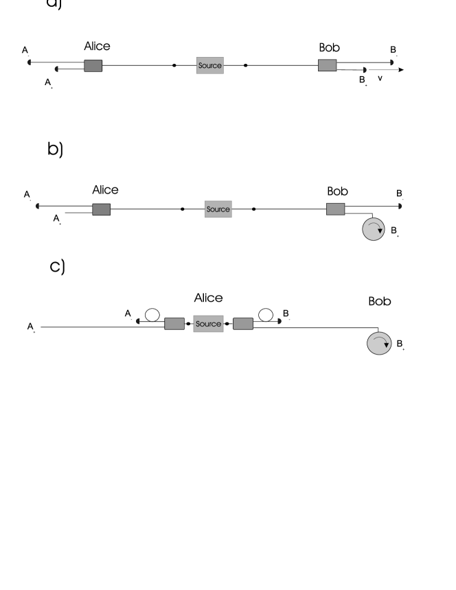
Figure 2: Schematic of the experimental arrangement with a moving detector (a). The linearly moving detector can be replaced by a rotating absorber (b). By placing the detectors close to the source (c), a breakdown of the nonlocal correlations could be exploited for superluminal signalling (see Appendix B).

Before, we have to discuss the question ”what is an observer?”, and ”where does a collapse of the wavefunction take place?”. Is it in the physicist’s mind, in the photon counter, or already at the beamsplitter or polarizer? The answer to such questions is usually not of practical relevance; however, for our kind of experiment the answer is crucial. It determines which part of the experiment should be moving and to which point the optical paths must have the same length. In this article, we assume that the effect occurs at the detector, when the irreversible transition from ”quantum” to ”classical” occurs. So we will have a situation like in Fig. 2a. Alice and Bob each have two detectors ( $A_{+},A_{-},B_{+},B_{-}$), two of which ($A_{+,}B_{+}$) are at precisely the same distance from the source. There are four possible outcomes with the corresponding probabilities. Normalization (conservation of particle number) imposes:

$$P_{A_{+},B_{+}}+P_{A_{+},B_{-}}+P_{A_{-},B_{+}}+P_{A_{-},B_{-}} = 1$$ (5)

$$P_{A_{+}}+P_{A_{-}} = 1$$ (6)

$$P_{B_{+}}+P_{B_{-}} = 1$$ (7)

The last two eqs. imply that if the photon is not detected by $A_{+}$, then it is necessarily detected by $A_{-}$ (assuming perfectly efficient detectors), and similarly for Bob’s detectors. Moreover, for maximally entangled states, as in our experiment, all 4 detectors have a probability $\frac{1}{2}$ of detecting a photon, independently of the interferometers settings:

$$P_{A_{+}}=P_{A_{-}}=P_{B_{+}}=P_{B_{-}}=\frac{1}{2}$$ (8)

With all detectors at rest, we can expect correlation of the events as a function of phase in the interferometers (or angles of the polarizers), as demonstrated in our previous experiment [14, 15]:

$$P_{A_{+},B_{+}}^{QM}=P_{A_{-},B_{-}}^{QM}=\frac{1+\cos(\delta_{a}+\delta_{b})}{2}\ \ {and\ }P_{A_{+},B_{-}}^{QM}=P_{A_{-},B_{+}}^{QM}=\frac{1-\cos(\delta_{a}+\delta_{b})}{2}$$ (9)

where the suffix $QM$ stands for Quantum Mechanics. If now, the detector $B_{+}$ is moving with respect to $A_{+}$ one might argue that correlations disappear (see the introduction and appendix A), i.e. that

$$P_{A_{+},B_{+}}^{bb}=const.=\frac{1}{4}$$ (10)

where the suffix $bb$ stands for before-before. Using (8) one has $P_{A_{+},B_{-}}=const.=\frac{1}{4}$ and, with help of (5) one deduces $P_{A_{-},B_{-}}=const.=\frac{1}{4}$. Consequently, one can test the prediction (10) by only looking at the coincidences between $A_{-}$ and $B_{-}$, the two detectors at rest! These detectors just have to be further away from the source than $A_{+}$ and $B_{+}$ to assure that the collapse occurs at $A_{+}$ or $B_{+}$.

The next question reads What is a detector?. One definition could be: it is any physical system in which the photon is irreversibly absorbed and transformed into a classical signal. The essential part is the irreversible process, the absorption of the photon in a solid and the transformation of its energy into heat. Since, as we have seen above, we don’t need to read the signal of the moving detector, the detector can be turned off or only consist of a non-fluorescent, black paint absorber (one can imagine that we could measure the temperature increase due to the absorption of the photon). Accordingly, detectors $A_{+}$ and $B_{+}$ can be just absorbing black surfaces The black surfaces provoke the collapse, even in the case that the photons go to the detectors! This considerably facilitates the experiment: First, we don’t need to identify precisely the absorbing layer of the photodiode. Second, the moving detector will be a spinning wheel. The rim of the wheel is painted black and the end of the optical fiber is pointed from outside on it (see Fig. 2b). Note that during the 50 $\mu$s time of flight of the photon from the source, the wheel’s edge moves by about 5 mm, thus our ”detector”, the molecules of the black paint, make in a good approximation a linear movement, defining the inertial reference frame. We don’t need electrical or optical contact, neither cooling of our spinning wheel as if a real detector was mounted.

We admit that the above argument is questionable and that it would be nicer to have real, moving photon counters that make ”click”. However, the argument is fair and it clearly turns a nightmare experiment into a feasible one. Let us also note that in their original work, Suarez and Scarani proposed, inspired by Bohm’s model, that the relevant device is the beamsplitter and not the detector. Thus, our experiment is not a test of their model.

3
Equalizing two fiber optical links

In order to perform the experiment, the source has to be set precisely at the center so that in the Geneva reference frames both photons are analyzed within a few ps, corresponding to about a millimeter over a fiber length of more then 18 km. In this section we describe how we achieved such a precision. Clearly, the chromatic dispersion which spread the photon wave-packet is also a serious concern.

We used installed telecom fibres and work with photons at wavelengths around 1300 nm. The relative group delay $\tau(\lambda)$ of a pulse, expressed in [ps/km], can be well fitted by the Sellmeier equation:

$$\tau(\lambda)=a\lambda^{2}+b\lambda^{-2}+c$$ (11)

The dispersion coefficient $D$ is defined as $D=\frac{d\tau}{d\lambda}$ has the units $ps/nm\cdot km$ and goes to zero at the zero dispersion wavelength $\lambda_{0}$. The parameter $S_{0}$ is the slope of the dispersion at $\lambda_{0}.$ For standard telecom fibers $\lambda_{0}$ is situated around 1310 nm and S₀ is close to 0.08 ps/km nm${}^{2}.$ Equation (11) can be rewritten in terms of $S_{0}=8a$ and $\lambda_{0}=\sqrt[4]{b/a}$:

$$\tau(\lambda)=\tau_{0}+\frac{S_{0}}{8}(\lambda-\frac{\lambda_{0}^{2}}{\lambda})^{2}\approx\tau_{0}+\frac{S_{0}}{2}(\lambda-\lambda_{0})^{2}$$ (12)

The first term (the group velocity delay) can be adjusted with a precison around 100 $\mu m$ (see below):

$$\tau(\lambda_{0}^{A})l^{A}\approx\tau(\lambda_{0}^{B})l^{B}$$ (13)

where $l^{A}$, $l^{B}$, $\lambda_{0}^{A}$ and $\lambda_{0}^{B}$ denote the lengths and the zero dispersion wavelengths of the fibres going to Alice and Bob, respectively. However, a simple estimate of the second term (chromatic dispersion) shows that a photon centered at $\lambda_{0}$ with a bandwidth of say 50 nm would suffer a spread of 245 ps per 10 km, which is much more than the maximum 10 ps target. Fortunately, working with photon pairs the major part of dispersion can be cancelled due to the energy correlation of the photons. Since $\omega_{p}=\omega_{s}+\omega_{i}$ the delays undergone by the signal and idler photons can be equalized:

$$S_{0}^{A}(\lambda^{A}-\lambda_{0}^{A})^{2}\approx S_{0}^{B}(\lambda^{B}-\lambda_{0}^{B})^{2}$$ (14)

For this we chose fibers such that $\lambda_{0}^{A}\approx\lambda_{0}^{B}$, $S_{0}^{A}\approx S_{0}^{B}$, and tuned the pumpwavelength to obtain $2\lambda_{p}=\frac{\lambda_{0}^{A}+\lambda_{0}^{B}}{2}$ (note, that eq. (12) is in function of $\lambda$ whereas the signal and idler photons are symmetric in $\omega$, but makes only a second order difference ). The difference in the group delay is then:

$$\delta t=l^{A}(\tau_{0}^{A}+\frac{S_{0}^{A}}{2}(\lambda^{A}-\lambda_{0}^{A})^{2})-l^{B}(\tau_{0}^{B}+\frac{S_{0}^{B}}{2}(\lambda^{B}-\lambda_{0}^{B})^{2})\approx 0$$ (15)

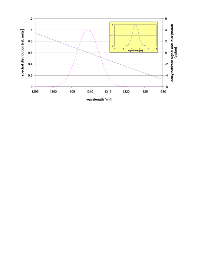
Figure 3: Spectral distribution of photon pairs (10nm FWHM interference filter centered at 1309.5nm ) and differential group delay for a fibre with $\lambda_{0}=1310nm$. Since the photons are centered close to $\lambda_{0},$ the most of dispersion induced delay between signal and idler photon is cancelled. The inset gives the distribution of time delay between idler and signal after 1 km of fibre.

Accordingly, in theory the quadratic term of (12) cancels and higher order terms are limiting. In practice, however, the precision with which one can measure and equalize the $\lambda_{0}$’s of the fibers determine $\delta t$. For a given spectral distribution of the photon pairs, determined by the transmission curve of an interference filter a corresponding distribution of the $\delta t$ in the group delay (see Fig. 3 ) is obtained. Table 1 gives two figures of merit for the temporal spread in ps per km for different deviations of center wavelength of the photon pairs from the mean zero dispersion wavelength ($2\lambda_{p}-\frac{\lambda_{0}^{A}+\lambda_{0}^{B}}{2}$) and bandwidths $\Delta\lambda$ (FWHM) of the filter. These are the $\Delta\tau_{\max}$ , the maximum difference of $\delta t$  for 95% of the photons that are within the $2\lambda_{p}\pm 2\sigma$ intervall and $\Delta\tau=2\sqrt{\int(\delta t(\lambda)-\overline{\delta t})^{2}p(\lambda)}$, the mean square deviation. This figures depend essentially on $\Delta\lambda$ and and in a first approximation not on $\lambda_{0}^{A}-\lambda_{0}^{B}$.

$2\lambda_{p}$	$\Delta\lambda=$ 10 nm	$\Delta\lambda=$ 40 nm	$\Delta\lambda=$ 70 nm
1309.0	0.95 (1.90) ps	3.3 (6.0) ps	4.4 (6.3) ps
1309.5	0.47 (0.93) ps	1.4 (2.2) ps	2.9 (2.6) ps
1310.0	0.013 (0.026) ps	0.8 (1.7) ps	6.7 (13.6) ps
1310.5	0.49 (0.99) ps	2.6 (5.5) ps	7.4 (15.8) ps
1311.0	0.97 (1.94) ps	4.5 (9.4) ps	0.95 (1.90) ps

Table 1: $\Delta\tau$ ($\Delta\tau_{\max})$ per km of fiber for different $\lambda_{p}$ and $\Delta\lambda$ (FWHM). $\lambda_{0}^{A}=\lambda_{0}^{B}=1310$ $nm.$

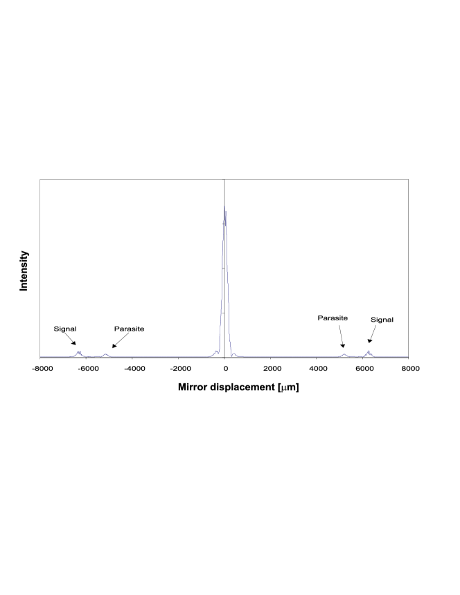
Figure 4: Typical scan of the low coherence interferometer. The signal is low due to the losses after 20 km of fibre (roundtrip). Nevertheless the position of peak can be determined with a precision of about 100$\mu m$. There is a parasite signal due to a reflection close to the source.

The chromatic dispersion was first measured with a commercial dispersion measurement apparatus (Anritsu ME 9301A) . Unfortunately, this apparatus revealed variations of the zero-dispersion wavelength of up to 2 nm. Next, we built up our own apparatus using a Delay generator (Standford 530), a pulsed LED, a tunable filter(JDS), an actively gated InGaAs APD and a time to amplitude converter (TAC, Tenelec TC836) [16]. We obtained a reproducibility of 0.1 nm and estimated the absolute error as 0.2 nm [17]. The length measurement was done in a first step with a home-made OTDR setup similar to that used for the dispersion measurement. It achieved a precision of 1-2 mm. In a second step we used a low coherence reflectometer (an interferometer with a scanning mirror) to determine the path difference to a precision of about 0.1 mm (Figure 4 shows a typical scan) . The standard resolution of about 20 $\mu m$ could not be obtained, since we had to reduce the spectral width of the LED with a tunable filter of 2 nm width (FWHM) in order to see interference. If the dispersion properties of two fibers were perfectly identical, the wavelength of the LED wouldn’t matter. We limited a possible shift of group delay by centering the filter at 2$\lambda_{p}$. We estimated the error of $2\lambda_{p}$ as 0.2 nm and we conservatively assumed that $2\lambda_{p}-\frac{\lambda_{0}^{A}+\lambda_{0}^{B}}{2}\approx 0.5$ $nm.$ For relative high differences $\lambda_{0}^{A}-\lambda_{0}^{B}\leq 1$ nm we then obtained a maximal shift of 0.1 ps/km what is negligable. Concerning the temporal spread of the photons we obtained according to Table 1 a spread $\Delta\tau$ of about 5 ps (for 10 km of fiber) if the bandwith of the downconverted photons is limited to 10 nm.

We performed our experiments between three Swisscom stations in Geneva and Bernex and Bellevue separated by 10.6 km bee-line. We obtained 9.53 km for link A (Geneva-Bernex) and 8.23 km for the link B (Geneva-Bellevue). We added 500 m dispersion shifted fiber to link A and 1.80 km of standard fiber to link B equalize roughly the length and as precisely as possible $\lambda_{0}$ and ended up with $\lambda_{0}^{A}=1313.0$ nm and $\lambda_{0}^{B}=1313.3$ nm. Two meters of fiber were mounted on a rail in order to adjust the length of link A by pulling or releasing the fiber. In Bellevue, the distance between the end of the fiber and the black wheel could also be adjusted within a range of a few mm.

4 Experimental setup

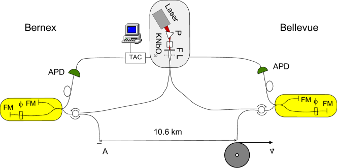
Figure 5: Schematic of the experiment.

The experimental setup was similar to our Franson-type Bell-experiment presented earlier in more detail [14], [15], see Fig. 5. The parametric downconversion source consisted essentially of a 655 nm diode laser (30mW Mitsubishi) with external grating and a KNbO₃ crystal (length 10 mm, cut at $\theta=33^{o}$). The analyzers were two Michelson interferometers with Faraday mirrors. We used optical circulators at the input ports in order to access to both outputs of the interferometers. At the circulator output ports we had our absorbers, a black scotch tape at A, the black wheel at B. These two surfaces were at exactly the same distance from the source. At the other output ports we connected our photon counters (passively quenched NEC Ge APD’s), making sure that they were further away from the source than the absorbers. Any detection triggered a laser pulse that was sent back to the source through another optical fibre. A TAC (Tenelec TC863) with Single Channel Analyzer selected the events with the right time interval, corresponding to two interfering possibilities when the photons take either both the short or both the long arm of the interferometers. We obtained typically 20 kcts/s single count rate plus 45 kcts/s dark count rates. This lead to a mean value of 10 coincidences per second. With the 10 nm FWHM interference filter inserted, we obtained 2 kcts singles and about 3 coincidences per second. The interferometers were temperature controlled. Interferometer A was kept at a constant temperature of 30^oC. The temperature of interferometer B scanned between 30.5 and 37.5 ⁰C. This produced a variation of the phase of about 10$\cdot 2\pi$ and therefore allowed us to record the coincidences as a function of the phase. The path length difference was measured to be equal when the temperature was $34^{o}$C. The wheel was a 20 cm diameter aluminium disk of 1 cm thickness directly driven by a brushless 250W DC motor (Maxon EC). It turned vertically at 10000 rpm leading to a tangent speed of 105m/s. The fiber pointed from the top on the blackened outer rim of the wheel. The wheel placed at Bellevue was oriented with a compass to make it run away or towards the other observer at Bernex.

5 Measurements and Results

We measured the path length difference between link A and B with the low coherence reflectometer. We found that the measurements were quite reproducible on short term, however, the length difference could vary by up to a few mm per hour. Actually we found that Bernex was drifting further away during the daytime, probably due to the fact that link A was more exposed to the daily temperature rise.

One possibility to test for the breakdown of the quantum correlation would be to measure the 2-photon interference visibility, move one absorber slightly closer, repeat the measurement and so on. As discussed above ( see Table 1), to limit dispersion effects and to obtain a good timing, we introduced a 10 nm (FWHM) interference bandpass filter after the source, reducing the coincidence count rate to some 3 cts/s. Hence to get a reasonable measurement statistics we needed some 100 sec integration time per measurement point, and some 10 points to see one interference fringe to determine the visibility, hence the measurement time was about 20 minutes. Since we couldn’t simultaneously measure the path difference and since the uncertainty in distance after 20 min was more than 1 mm, it was difficult to make a scan in distance with a spatial resolution better than 1mm. So we decided to renounce to a manual distance scan and to take profit of the natural temperature induced drift. This drift proved to be monotonous in one sense during the day and in the other sense during the night. So we almost aligned the paths knowing that due to daily the drift will perfectly aligned in certain moment later in time. We started then to record the interference fringes of the coincidences by homogeneously varying the phase. Finally we confirmed with a second position measurement after a few hours that the path lengths really passed through the presumed equilibrium. Then, we analyzed the interference fringes and looked for periods of reduced visibilities during the measurement.

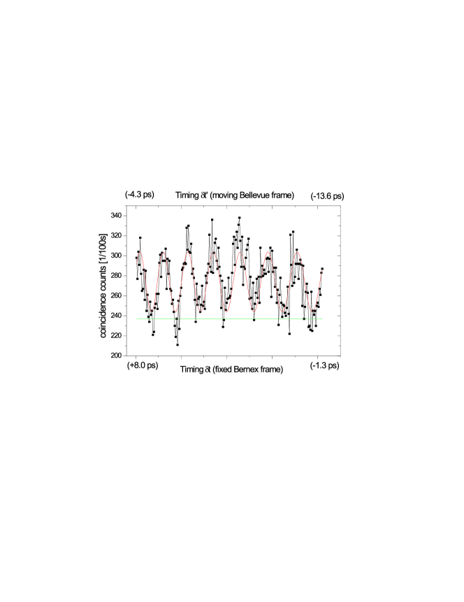
Figure 6: 2-photon interference fringes measured over 6 h while the optical distance to Bernex was slowly overpassing that to Bellevue. Positive time values indicate that the detection occued first in Bernex. According the moving reference frame, dectection occured first in Bellvue over the whole scan range. Despite this different chronology of the events no change in the visibility can be observed.

Figure 6 shows typical data taken over 6 hours while the optical link to Bernex lengthened by 2 mm with respect to the one to Bellevue. The difference of the optical path lenghts, expressed in $\delta t$, was varying from + 8 to -1.3 ps. Positive values mean that the detections occured first in Bernex. In the moving Bellevue reference frame the detections happened first in Bellevue over the entire scan range, as indicated by the negative values of $\delta t^{\prime}$on the upper time scale. Despite this different time ordering no reduced visibility is observed. Inevitably, the curves show high statistical fluctuations due to the low count rate. In spite of this, one can state that the visibilitiy of the two photon interferogram remains constant. Especially, a reduced visibility over a scan span of 1 mm (corresponding to 5 ps) should easily be noticed. After substraction of the 237$\pm 5$ cts/100s accidental coincidences, the fit of Fig 2 shows a constant fringe visibility of 83%, large enough for a violation of Bell’s inequality. Note however, that hidden variables are no issue in this work.

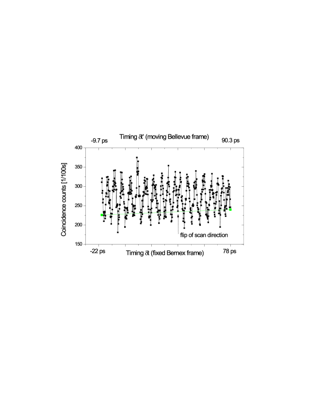
Figure 7: 2-photon interference fringes measured over 14 h while the optical distance to Bellevue was slowly overpassing that to Bernex. At some time we have negative values in fixed Bernex frame, indicating that the detection occurs first in Bellevue, and positive values in the moving Bellvue frame, indicating that detection detection occurs first in Bernex. Despite this after-after constellation no reduced visibility can be seen.

Figure 7 shows a scan over a longer period (14 hours overnight) and larger scan range. This time the wheel was turning in the other direction (towards Bernex) and the optical link to Bernex shortened by 20mm. Comparing the two time scales we find a period in the left part of the scan where we have negative values below and positive ones above. Hence, we have again a different time ordering, now both observers suppose to make the measurement after the other. Again, there is no evident drop of the visibility over a period of 10 ps, i.e. over roughly two fringes, assuming a rather homogenous scan rate. This scan over such a long period shows the problems of the experiment. The period of the fringes can vary due to small drifts of the pump laser frequency. The photon counters may have varying efficiency and dark count level. The slowly mounting line of accidentals is due to the fact that we measured higher darkcount rates at the end of the experiment, possibly due to increased temperature of one of the detector, since there was little liquid nitrogen left. Finally, the visibility may slightly decrease due a drift of the coincidence window discriminating the three temporal peaks of the Franson interferogram. Moreover, during a long scan some artefact are probable, as the the considerably higher peak after one third of the scan (sombody switching the lights on in the Swissom station?). The arrow indicates the moment when the scan of the phase by scanning the temperature of the Bernex interferometer changed the direction. Altogether we recorded over 20 tracks similar to those presented in Fig. 6 and 7 and no reproducable effect on the visibility could be determined.

The Figures 6 and 7 can also be used to estimate the lower bound for the speed of quantum information. At a certain time the two paths are perfectely equal and the lower bound could be arbitrarly high. In practice two factors limit this lower bound. First, we assume that at least one fringe should vanish to be able to state a reduced visibility. In Fig. 6, for instance, we observe 7 fringes for 10 ps delay. So the minimum time difference is say 1.5 ps. The second factor, the temporal spread of the photons, is the determining one in our case. We estimate it to be smaller than 5 ps. The lower speed limit becomes then:

$$\frac{10.6\ km}{\ 5\ ps}\approx 2\cdot 10^{15}\frac{m}{s}=\frac{2}{3}10^{7}c$$ (16)

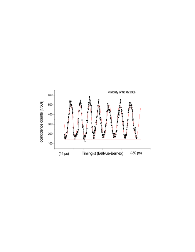
Figure 8: 2-photon interference fringes measured with two aligned detectors over 5h30 while the optical distance to Bernex was slowly overpassing that to Bellevue. At a certain time the two fixed detectors are at exactly the same distance from source.

We also performed measurements with two Ge APD’s precisely aligned instead of the absorbing surfaces showing the same evidence. Further we removed the interference filter limiting the bandwith. The curve (Fig. 8) shows a high visibility over the whole scan range. However, in this case the photons have approximately 70 nm FWHM and we have to assume some 100 ps spread. You may feel more confident with this measurement, since only real detectors and no black surfaces are involved. However, the moment of the collapse of the wavefunction is better defined in a black surface. We can assume that the lifetime of excited levels of molecules of the paint is very short, i.e. that the absorbed photon energy is transformed to heat within less than 1 ps. In contrary, APD photon counters have a time jitter in the order of 300 ps, to some extent due to the fact that created electron-hole pair in the absorbing takes more or less time to diffuse to the multiplying region. But it’s only there, where the irreversible proces from a quantum state to a macroscopic state occurs, which is our definition of the collapse. So, in fact we have an additional uncertainty in the timing of the collapse in the order of 100 ps, the same order of magnitude as the dispersion induced spread. The lower speed limit becomes then $\frac{1}{3}10^{6}c.$

One can assume that the collapse happens in some preferred frame, which is not the frame of Geneva-Bellevue-Bernex. A reasonable candidate is the frame of the cosmic background radiation. An analysis of our data shows that for this frame a lower speed limit for the quantum information of 1.5x10${}^{4}c$ can be given [25, 24].

6 Conclusions

Entanglement is the main resource of Quantum Information Processing and is at the core of the uneasiness many people face with the quantum world. It thus deserves to be widely studied, both theoretically and experimentally. In this work we have presented results from a first experiment in which both the relativity of timing and entanglement of spatially separated systems are central. Indeed, in the tested configuration the time ordering of the two measurements of the quantum systems depend on the reference frame defined by the two ”measurement apparatuses”. Each apparatus consists of an interferometer with two outputs. One output is connected to a standard photon counting detector, while the other output is connected to a ”passive detector”, i.e. a detector which irreversibly absorbs the photon, but spread the information in the environment without registering a signal in a form readable for humans. We have argued that such ”passive detectors” have the same physical effect on the photon and that the result of this effect can be read of the active detector at the other output (if the photon does not show up at one output, it is at the other output). Furthermore we have argued that the crucial part of each measurement apparatus is the detector which encounters the photon’s wave-packet first. Hence, we arranged the experiment such that the crucial parts of each measurement are the ”passive detectors” and that these are in relative motion such that the time ordering of the impacts of the two entangled photons on them depends on the reference frame defined by these moving ”passive detectors”.

The results are always in accordance with QM, re-enforcing our confidence in the possibility to base future understanding of our world and future technology on quantum principles. To achieve our experiment we had to set the 2-photon source very precisely at the center between the two measurements, i.e. the two impacts on the detectors were simultaneous in the Geneva reference frame to within 5 ps. This sets a lower bound on the speed on quantum information to $10^{7}$c, i.e. seven orders of magnitude larger than the speed of light.

The description of ”quantum measurements” is notoriously difficult and controversial. The results we have presented make it even more delicate to give a realistic description with ”real collapses”. On the other side, the reasoning we have followed opens new ways to test quantum mechanics and its weird description of ”measurements”. The assumptions we made to achieve this first experiment can and should be criticized. For instance, the assumption that the detector is the crucial step in a measurement is at odds with the idea that the collapse takes place in the reference frame determines by this detector, as discussed in appendix B. But at least these assumptions lead to a feasible experiment and will hopefully trigger new proposals.

It is a great time for quantum physics. Both its foundations and its potential applications are deeply explored by a growing community of physicists, mathematicians, computer scientists and philosophers. We explored experimentally some of the most counter intuitive predictions of quantum theory, stressing the tension with relativity. Our results contribute to the renewed interest for experimental challenges to the interpretation of quantum mechanics and is relevant for the realist-positivist debate. ”Experimental metaphysics” questions [18] like ”what about the concept of states?”, ”the concept of causalities?” will have to be (re)considered taking into account the results presented in this article. For example, our results make it more difficult to view the ”projection postulate” as a compact description of a real physical phenomenon [19, 20].

Appendices

Appendix A Probabilities for moving observers

Let P and Q denote two projector acting on spatially separated Alice and Bob systems, respectively. We shall use the identification $P\approx P\otimes\leavevmode\hbox{\small 1\kern-3.8pt\normalsize 1}$ and $\leavevmode\hbox{\small 1\kern-3.8pt\normalsize 1}\otimes Q\approx Q$. If the measurements corresponding to P and Q are either before-after or after-before, then the test-theory predicts the same probability as standard QM, with $\psi\in{\cal H}_{1}\otimes{\cal H}_{2}$ the usual quantum state:

$$Prob(++|b-a)=<Q>_{P\psi}<P>_{\psi}$$ (17)

$$= Prob(++|a-b)=<P>_{Q\psi}<Q>_{\psi}$$ (18)

$$= Prob(++|QM)=<P\otimes Q>_{\psi}$$ (19)

If, however, both measurements are before we postulate (inspired by Suarez & Scarani):

$$Prob(++|b-b)=<P>_{\psi}<Q>_{\psi}\neq Prob(++|QM)$$ (20)

The case after-after is the most delicate to guess. Inspired by Suarez’ intuition that in such a case each particle tries to guess what the other would have done if it were before (as if the information from the other particle would have got lost), we try the following postulate:

$$Prob(++|a-a) = <P\otimes Q>_{\psi}<P>_{Q\psi}<Q>_{P\psi}$$

$$+< P\otimes Q^{\perp}>_{\psi}<P>_{Q^{\perp}\psi}<Q>_{P\psi}$$

$$+< P^{\perp}\otimes Q>_{\psi}<P>_{Q\psi}<Q>_{P^{\perp}\psi}$$

$$+< P^{\perp}\otimes Q^{\perp}>_{\psi}<P>_{Q^{\perp}\psi}<Q>_{P^{\perp}\psi}$$

$$\neq Prob(++|QM)$$

where $<P>_{Q\psi}\equiv\frac{<Q\psi|P|Q\psi>}{<Q\psi|Q\psi>}=\frac{<P\otimes Q>_{\psi}}{<Q>_{\psi}}$. The idea is that Alice system evaluate the projector P in either the state $Q\psi$ or $Q^{\perp}\psi$ depending on its guess of Bob’ system outcome. The situation is clearly symmetric. Hence the 4 alternatives are weighted according to the standard outcome probabilities (it does not matter whether it is Alice who guesses that Bob was first, or whether it is Bob who assumes that Alice was first). In (A each line corresponds to one possible guess, the first term giving the corresponding guess probability (e.g. $<P\otimes Q>_{\psi}$ for both guessing that theother had a positive outcom) and the two last terms the corresponding outcomes probabilities (e.g. $<P>_{Q\psi}<Q>_{P\psi}$).

The other probabilities for the after-after configuration follow: e.g. $Prob(+-|a-a$ obtains from (A) by replacing $Q$ with $Q^{\perp}$.

A first consistency check is for product states: if $\psi=\alpha\otimes\beta$, then from (A) follows $Prob(++|a-a)=<P>_{\alpha}<Q>_{\beta}$.

As second consistency check let us compute:

$$Prob(++|a-a) + Prob(+-|a-a)=$$

$$= <P\otimes Q>_{\psi}(<P>_{Q\psi}<Q>_{P\psi}+<P>_{Q\psi}<Q^{\perp}>_{P\psi})$$

$$+ <P\otimes Q^{\perp}>_{\psi}(<P>_{Q^{\perp}\psi}<Q>_{P\psi}+<P>_{Q^{\perp}\psi}<Q^{\perp}>_{P\psi})$$

$$+ <P^{\perp}\otimes Q>_{\psi}(<P>_{Q\psi}<Q>_{P^{\perp}\psi}+<P>_{Q\psi}<Q^{\perp}>_{P^{\perp}\psi})$$

$$+ <P^{\perp}\otimes Q^{\perp}>_{\psi}(<P>_{Q^{\perp}\psi}<Q>_{P^{\perp}\psi}+<P>_{Q^{\perp}\psi}<Q^{\perp}>_{P^{\perp}\psi})$$

$$= <P\otimes Q>_{\psi}<P>_{Q\psi}+<P\otimes Q^{\perp}>_{\psi}<P>_{Q^{\perp}\psi}$$

$$+ <P^{\perp}\otimes Q>_{\psi}<P>_{Q\psi}+<P^{\perp}\otimes Q^{\perp}>_{\psi}<P>_{Q^{\perp}\psi}$$ (23)

$$= <Q>_{\psi}<P>_{Q\psi}+<Q^{\perp}>_{\psi}<P>_{Q^{\perp}\psi}$$ (24)

$$= <P>_{\psi}$$ (25)

Accordingly, the local probabilities follow the standard laws, as they should!

We compute now the correlation function

$$E(P,Q) = Prob(++)+Prob(--)-Prob(+-)-Prob(-+)$$

$$= <P\otimes Q>_{\psi}<\sigma_{P}>_{Q\psi}<\sigma_{Q}>_{P\psi}$$

$$+< P\otimes Q^{\perp}>_{\psi}<\sigma_{P}>_{Q^{\perp}\psi}<\sigma_{Q}>_{P\psi}$$

$$+< P^{\perp}\otimes Q>_{\psi}<\sigma_{P}>_{Q\psi}<\sigma_{Q}>_{P^{\perp}\psi}$$

$$+< P^{\perp}\otimes Q^{\perp}>_{\psi}<\sigma_{P}>_{Q^{\perp}\psi}<\sigma_{Q}>_{P^{\perp}\psi}$$ (27)

where $\sigma_{P}\equiv P-P^{\perp}$ and $\sigma_{Q}\equiv Q-Q^{\perp}$. Let us illustrate this conjecture for the singlet state with $\sigma_{P}=\vec{a}\vec{\sigma}$ and $\sigma_{Q}=\vec{b}\vec{\sigma}$:

$$E(\vec{a},\vec{b}) = \frac{1-\vec{a}\vec{b}}{4}\left((\vec{a}\vec{b})^{2}+(-\vec{a}\vec{b})^{2}\right)$$ (28)

$$+ \frac{1+\vec{a}\vec{b}}{4}\left((\vec{a}\vec{b})(-\vec{a}\vec{b})+(-\vec{a}\vec{b})(\vec{a}\vec{b})\right)$$

$$= -(\vec{a}\vec{b})^{3}$$ (29)

This may be more difficult to distinguish experimentally from the before-before conjecture. Note that if $\vec{a}$ and $\vec{b}$ are parallel (or anti-parallel), then the maximal anti-correlation (correlation) are predicted. This is in accordance with the idea that each particle guesses the other’s output.

Appendix B Detectors as choice device and super-luminal communication

In this appendix we elaborate on the assumption that the collapse (i.e. the outcome of the measurement) is determined by the detector. We show that using this assumption one can device a situation in which quantum nonlocality could be activated, that is use to signal at arbitrary high speeds.

Let us return to figures 1. Why not leave the interferometers close to the source and just put the absorbing surfaces at a distance. The detectors can then also stay by the source, provided a long fiber spool is inserted to ensure that the detections occur after the collapse (see Fig. 1c). So we are looking at coincidences between two detectors side by side. When the wheel is turning at Bob’s the correlation should disappear. Since Bob can be very far away from the source and the detection of photons must occur just shortly after the potential arrival of the photons at Alice and Bob. Bob could, by switching on and off the wheel, send signals back to the source at superluminal speed.

The peaceful coexistence between quantum mechanics and relativity [3] is one of the most remarkable facts of physics! It is notoriously difficult to modify quantum mechanics without activating quantum non-locality, hence without breaking this peaceful co-existence [21, 22]. Weinberg has argued on this base that quantum mechanics is part of the final theory [23]! In this appendix we see once again that a proposed modification to basic quantum mechanics requires also a radical modification of relativity. However, it is possible that it is not the detector that triggers the collapse. The photons could take the decision already at the beamsplitter and go out through one output port, like in the Bohm-de-Bloglie pilot wave picture [26] (which much inspired Suarez). With the beam-splitter as choice-device superluminal signaling is not possible (to our knowledge). A corresponding experimental test would be more demanding, a beam-splitter would have to be in motion. A clever way-out could be the use of an acousto-optical modulator representing a beam-splitter moving with the speed of the acoustic wave. We are working on such an experiment.

Appendix C Figures

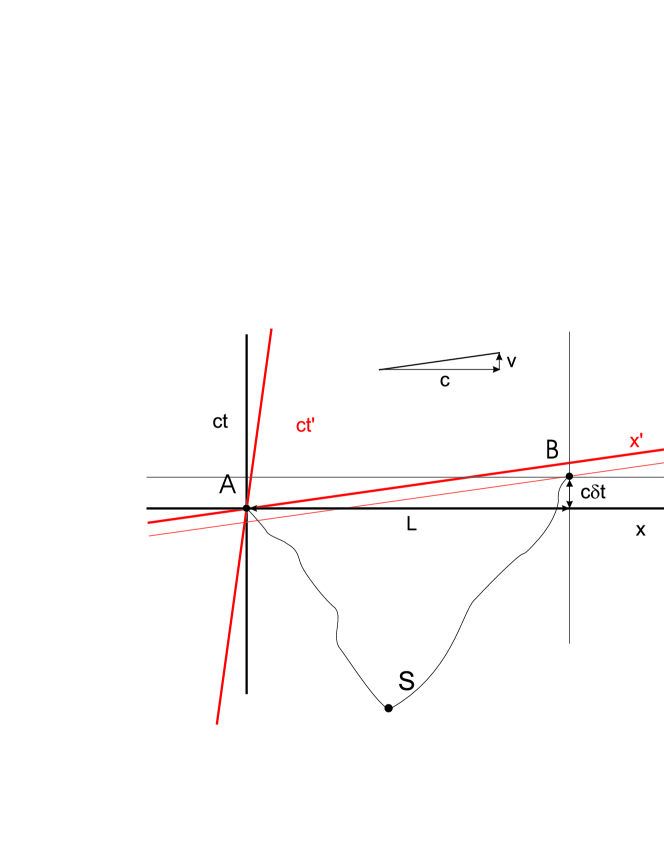
Figure 1: Space-time diagram of a Bell experiment with moving observer. In the referential frame of the moving observer (x’,ct’) event B happens before event A. Note that the source does not have to be located in the middle between the two detectors. Only the optical path lengths must be the same.

References

- [1] A. Einstein, B. Podolsky & N. Rosen, Can quantum-mechanical description of physical reality be considered complete?, Phys. Rev. 47, 777-780 (1935)
- [2] J. S. Bell, Physics 1, On the Einstein Podolsky Rosen paradox, 195-200 (1964).
- [3] Shimony, A., in Foundations of Quantum Mechanics in the Light of New Technology, ed. Kamefuchi, S., (Phys. Soc. Japan, Tokyo, 1983).
- [4] Aharonov, Y., & Albert, D. Z., Can we make sense out of the measurement process in relativistic quantum mechanics, Phys. Rev. D 24, 359-370 (1981), ibid 29, 228, 1984.
- [5] Hardy, L., Quantum mechanics, local realistic theories, and Lorentz-invariant realistic theories, Phys. Rev. Lett. 68, 2981-2984 (1992).
- [6] I.C. Percival, Quantum Transfer Functions, weak nonlocality and relativity, Phys. Lett. A 244, 495-501, 1990 & Quantum measurement brakes Lorentz symmetry, quant-ph 9906005
- [7] G.C. Ghirardi, R. Grassi and Ph. Pearle, Found.Phys. 20, 1271, 1990.
- [8] P. Busch, P. J. Lahti, and P. Mittelstaedt, The Quantum Theory of Measurement, Springer, Berlin, 1991.
- [9] J.M. Jauch, Foundations of Quantum Mechanics, Addison-Wesley, Reading Mass., 1968.
- [10] C. Piron, Foundations of Quantum Physics, W.A.Benjamin inc., Reading, Mass., 1976.
- [11] A. Shimony, in Quantum concepts of space and time, eds R. Penrose and C. Isham, pp 182-203, Oxford University Press, 1986.
- [12] D. Deutsch, The fabric of reality, Penguin Press 1997
- [13] Suarez, A., & Scarani, V., Does entanglement depend on the timing of the impacts on the beam-splitters?, Phys. Lett. A 232, 9-24 (1997).
- [14] W. Tittel, J. Brendel, N. Gisin, and H. Zbinden,Violation of Bell inequalities by photons more than 10km apart, Phys. Rev. Lett. 81 (17), 3563-3566 (1998).
- [15] W. Tittel, J. Brendel, N. Gisin, H. Zbinden, Long-distance Bell-type tests using energy-time entangled photons, Phys. Rev. Lett. 82 (12), 2594-2597 (1999).
- [16] GAP sells prototypes based on an improved setup with Bragg-gratings instead of the tunable filter.
- [17] J. Brendel, H. Zbinden and N. Gisin, Optical Fiber Measurement Conference OFMC’99, pp 12-17, Eds Ch. Boisrobert and E. Tanguy (Univeristé de Nantes), Nantes, September 1999.
- [18] Experimental Metaphysics, Eds Cohen, R.S., Horne, M. & Stachel, J., (Kluwer Acad. Pub., Dordrecht, 1997).
- [19] Pearle Ph., Suppose the state vector is real: the description and consequences of dynamical reduction, Annals NY Acad. Sciences 480, 539-552 (1985).
- [20] Gisin N., Stochastic Quantum Dynamics and Relativity, Helv. Phys. Acta 62, 363-371 (1989).
- [21] N. Gisin, Phys. Lett. A 143, 1-2, 1990.
- [22] M. Czachor, Found. Phys. Lett. 4, 351, 1991.
- [23] Weinberg, S. 1993 Dreams of a Final Theory, Hutchinson Radius, London.
- [24] H. Zbinden, J. Brendel, W. Tittel, N. Gisin, quant-ph/0002031
- [25] V. Scarani, N. Gisin, W. Tittel, H. Zbinden, The speed of quantum information and the preferred frame: Analysis of experimental data, quant-ph/0007008.
- [26] J.S. Bell, Foundations of Physics 12, 989-999 (1982).