Continuous optical loading of a Bose–Einstein Condensate

Abstract

The continuous pumping of atoms into a Bose–Einstein condensate via spontaneous emission from a thermal reservoir is analyzed. We consider the case of atoms with a three–level $\Lambda$ scheme, in which one of the atomic transitions has a very much shorter life–time than the other one. We found that in such scenario the photon reabsorption in dense clouds can be considered negligible. If in addition inelastic processes can be neglected, we find that optical pumping can be used to continuously load and refill Bose–Einstein condensates, i.e. provides a possible way to achieve a continuous atom laser.

I Introduction

During the last years, the fruitful combination of laser–cooling [1] and evaporative cooling [2] has allowed the experimental achievement of the Bose–Einstein condensation (BEC) in trapped weakly interacting alkali gases. Such remarkable achievement has stimulated an enormous interest [3]. The subsequent efforts mainly concentrated on two different areas. On one side, the BEC offers an extraordinary opportunity to test condensed matter and low–temperature phenomena. In this respect, very recently several striking results have been reported concerning superfluidity phenomena [4, 5] and generation and dynamics of vortices [6, 7] and dark–solitons [8, 9]. On the other hand, the macroscopically occupied matter wave can be manipulated by atom optical elements, that can be combined to provide new tools for precision experiments [10]. Besides passive optical elements recently also active elements, that provide phase coherent gain have been demonstrated [11]. Also a new field, called Non–Linear Atom Optics (NLAO), has rapidly developed during the last years. Several remarkable experiments have been recently reported in this area, as reflection of BEC from an optical mirror[12] and four–wave mixing [13] of matter waves.

Among the results related to BEC and NLAO, one of the most important experimental achievements was the realization of an Atom Laser. As a coherent source of matter waves, the atom laser will lead to new applications in atom optics. Its impact in the field is comparable to the one of light lasers in light optics. The first realization of an atom laser was achieved via pulsed rf-outcoupling from a BEC [14]. The coherent character of the source was demonstrated in a landmark experiment [15], in which two atom–laser pulses where overlapped, showing a clear interference pattern.

Since this first realization, several groups have build atom lasers using (quasi-) continuous outcoupling from the BEC, either by using rf fields [16, 17], or by employing Raman pulses [18]. However, the continuous outcoupling represents just a half way towards a cw atom laser. The continuous loading of the condensate still remains to be incorporated in experiments. Without a continuous refilling of the BEC, the atom laser output lasts only as long as some atoms in the BEC are kept. Like in the development of light lasers the availability of cw atom lasers would open the way to ”high power” and precision applications.

Two different physical mechanisms could provide a continuous pumping into a condensate. On one hand, the collisional mechanisms [19], in which two non–condensed atoms from a reservoir collide, and as a result one is pumped into the condensate, whereas the other carries most of the energy and is evaporated. On the other hand, the optical pumping of reservoir atoms into a BEC via spontaneous emission processes has been also proposed [20]. If this reservoir could be filled in a (quasi-) continuous way by laser cooling techniques, one would benefit from the large cooling efficiency of laser cooling compared to evaporative cooling, allowing for a considerable increase in atomic flux produced by an atom laser. For the latter, it is crucial that the spontaneously emitted photons cannot be reabsorbed, because otherwise a heating is introduced in the system, and BEC can be neither achieved nor maintained [21].

Several possible dynamical and geometrical solutions for the reabsorption problem have been proposed during the last few years. The geometrical proposals are based on the reduction of the dimensionality of the traps [23, 21]. It is easy to understand that assuming that the reabsorption cross section for trapped atoms is the same as in free space, i.e. $\simeq 1/k_{L}^{2}$, the significance of reabsorptions increases with the dimensionality, in such a way that the reabsorptions should not cause any problem in one dimension, have to be carefully considered in two dimensions, and forbid condensation in three dimensions. Therefore, cigar-shape and disc-shape traps have been suggested. However even severe deformations of the trap do not allow more than modest reductions of the reabsorption heating [24]. Other suggestion consists in using a strongly confining trap with a frequency $\omega\simeq\omega_{R}$. In this case, it has been proved [25] that in two atom systems the relative role of reabsorption in such a trap can be significantly reduced. It is, however, not clear whether this result would hold for many atom systems. Another promising remedy against reabsorption heating employs the dependence of the reabsorption probability for trapped atoms on the fluorescence rate $\gamma$, which can be adjusted at will in dark state cooling [24]. In particular, in the interesting regime in which $\gamma$ is much smaller than the trap frequency $\omega$, i.e. in the so called Festina Lente limit [26], the reabsorption processes, in which the atoms change energy and undergo heating, are practically completely suppressed. However due to the slow time constants in this approach the cooling efficiency is greatly reduced. Another reabsorption remedy could be provided by the destructive quantum interference of the negative effects of the photon reabsorption in the, so–called, Bosonic–Accumulation Regime [27].

In this paper, we concentrate on the continuous optical pumping into a BEC. The paper is divided in two different parts. In the first part we present a new scenario in which the reabsorption is suppressed, in much less restrictive conditions than that of Festina Lente regime, i.e. without reducing the cooling efficiency. In this scenario, an atom possesses an accessible three level $\Lambda$ scheme, in which one of the atomic transitions decays much faster than the other. By employing Master Equation (ME) techniques, we show that the dangerous reabsorptions of photons on the slow transition are suppressed because the respective coherences are destroyed due to the decay via the fast transition. By dangerous we mean here those reabsorptions that may lead to undesired heating of the system. Since the dangerous reabsorptions are not present, this scheme can be employed to continuously pump atoms into the lower level of the slower transition. In the second part of the paper we analyze the dynamics of such pumping in the presence of atom–atom collisions, and show that the combination of elastic collisions (evaporative cooling), and bosonic enhancement of the spontaneous emission, can create a condensate, and refill it in the presence of outcoupling or losses. Therefore, this scheme could be considered as a possible way towards a continuously loaded atom laser. As a possible experimental realization we consider laser cooled Chromium, but the ideas can be generalized to any atom that provides an asymmetric three–level system.

The structure of the paper is as follows. In Sec. II we introduce the physical model, as well as the quantum ME that determines the loading dynamics. In Sec. III we introduce the so–called Branching Ratio Expansion (BRE), which allows us to analyze the hierarchy of processes which occur in the system. In Sec. IV we analyze in detail the suppression of the reabsorption effects. Sec. V is devoted to the treatment of the atom–atom collisions. In Sec. VI we present the numerical Monte Carlo results of the loading dynamics. Finally, we summarize some conclusions in Sec. VII.

II Model

We consider the case of atoms with an accessible three level $\Lambda$ system (see Fig. 1), formed by the levels $|r\rangle$, $|e\rangle$ and $|g\rangle$. The atoms are trapped in an isotropic harmonic trap which, depending of the internal state of the atoms, has frequencies $\omega_{r}$, $\omega_{e}$ and $\omega_{g}$, respectively. This could be, for instance, the case of Chromium ⁵²Cr, in which the electronic levels would be ⁷S₃, ⁷P₄, and ⁵D₄, respectively. The transition $|r\rangle\leftrightarrow|e\rangle$ is assumed to be driven by a laser, which has a Rabi frequency $\Omega$. The spontaneous emission frequencies associated with the transitions $|r\rangle\leftrightarrow|e\rangle$ and $|g\rangle\leftrightarrow|e\rangle$ are, respectively, $\gamma_{er}$ and $\gamma_{eg}$, such that $\gamma_{er}\gg\gamma_{eg}$. In the case of ⁵²Cr, $\gamma_{er}=2\pi\times 5$MHz $\gg\gamma_{eg}=2\pi\times 30$Hz. The branching ratio $\epsilon\equiv\gamma_{eg}/\gamma_{er}$ is therefore very small ($\sim 10^{-5}$ in ⁵²Cr). The fact that $\epsilon\ll 1$, will lead to the suppression of the reabsorption of scattered photons.

FIG. 1.: Atomic scheme considered throughout the paper.

In this section, we shall not consider the collisions between the atoms in the $|g\rangle$ state. Such collisions are introduced in our formalism in Sec. V. In the following we take $\hbar=c=1$ for simplicity. Let us introduce the annihilation and creation operators of atoms in the $|r\rangle$, $|e\rangle$ and $|g\rangle$ states and in the trap levels $s$, $l$, and $m$ which we shall call $r_{s},r_{s}^{{\dagger}}$, $e_{l},e_{l}^{{\dagger}}$, and $g_{m},g_{m}^{{\dagger}}$. These operators fulfill the standard bosonic commutation relations.

The Hamiltonian which describes the coupling of the system of bosons to the laser field, as well as to the vacuum electromagnetic modes is of the form:

$$\hat{H}=\hat{H}_{0}+\hat{H}_{er}+\hat{H}_{af}^{er}+\hat{H}_{af}^{eg}+\hat{H}_{f},$$ (1)

with the following terms:

• Free atomic Hamiltonian (describing internal and center–of–mass degrees of freedom):

  $$\hat{H}_{0}=\sum_{s}\omega_{s}^{r}r_{s}^{{\dagger}}r_{s}+\sum_{l}(\omega_{l}^{e}+\omega_{0})e_{l}^{{\dagger}}e_{l}+$$ (2)

  $$\sum_{s}\omega_{m}^{g}g_{m}^{{\dagger}}g_{m},$$ (3)

  with $\omega_{s}^{r}$, $\omega_{l}^{e}$ and $\omega_{m}^{g}$, denoting the energies of the level $s$ of the $|r\rangle$ trap, the level $l$ of the $|e\rangle$ trap, and the level $m$ of the $|g\rangle$ trap, respectively. $\omega_{0}$ is the transition frequency between $|r\rangle$ and $|e\rangle$.

• Interactions of the laser quasiresonant with the transition $|r\rangle\leftrightarrow|e\rangle$:

  $$H_{er}=\frac{\Omega}{2}\sum_{l,s}\eta_{l,s}e^{-i\omega_{L}t}e_{l}^{{\dagger}}r_{s}+h.c.,$$ (4)

  where $\eta_{l,s}$ is the Franck–Condon factor which describes the transition between a level $s$ of the $|r\rangle$ trap, and a level $l$ of the $|e\rangle$ trap, and $\omega_{L}$ is the frequency of the applied laser.

• Spontaneous emission processes $|e\rangle\rightarrow|r\rangle$:

  $$\hat{H}_{af}^{er}=-i\sum_{l,s}\sum_{\mu}\int d^{3}\vec{k}\sqrt{\frac{k}{2\epsilon_{0}(2\pi)^{3}}}(\vec{d}_{er}\cdot\vec{\epsilon}_{\vec{k}\mu})$$ (5)

  $$\times\eta_{ls}(\vec{k})e_{l}^{{\dagger}}r_{s}a_{\vec{k}\mu}+h.c.,$$ (6)

  where where $a_{\vec{k}\mu}$, $a_{\vec{k}\mu}^{{\dagger}}$ are the annihilation and the creation operators of a vacuum photon characterized by a wavevector $\vec{k}$ and a polarization $\mu$, with polarization vector $\vec{\epsilon}_{\vec{k}\mu}$; $\vec{d}_{er}$ is the dipole vector of the transition $|r\rangle\leftrightarrow|e\rangle$.

• Spontaneous emission $|e\rangle\rightarrow|g\rangle$:

  $$\hat{H}_{af}^{eg}=-i\sum_{l,m}\sum_{\mu}\int d^{3}\vec{k}\sqrt{\frac{k}{2\epsilon_{0}(2\pi)^{3}}}(\vec{d}_{eg}\cdot\vec{\epsilon}_{\vec{k}\mu})$$ (7)

  $$\times\eta_{lm}(\vec{k})e_{l}^{{\dagger}}g_{m}a_{\vec{k}\mu}+h.c.,$$ (8)

  where $d_{eg}$ is the dipole vector of the transition $|g\rangle\leftrightarrow|e\rangle$.

• Free Hamiltonian of the electromagnetic (EM) field

  $$\hat{H}_{f}=\sum_{\mu}\int d^{3}\vec{k}ka_{\vec{k}\mu}.$$ (9)

Starting from the Hamiltonian (1), one can trace the full density matrix of the system over the vacuum modes of the EM field. Using standard methods of quantum stochastic processes [28], one can derive then the Quantum Master Equation in Born–Markov approximation [29]. In principle such ME fully describes all the processes which happen in the system, including eventual reabsorptions in the fast transition $|e\rangle\rightarrow|r\rangle$. However, for simplicity of the analysis we shall consider the case in which we can neglect the reabsorption phenomena for the reservoir atoms ($|e\rangle$ and $|r\rangle$). Although what follows is true also in presence of those reabsorptions, the approximation will allow us to concentrate on the much simpler problem of the pumping of a single atom from the reservoir $\{|e\rangle,|r\rangle\}$ into the $|g\rangle$ trap, where of course, collective phenomena are important, and therefore taken into account. In this case, the ME takes the form

$$\dot{\rho}=-iH_{eff}\rho+i\rho H_{eff}+{\cal J}\rho,$$ (10)

where $\rho$ is the density matrix, $H_{eff}=H_{eff}^{(0)}+H_{eff}^{(1)}$ and ${\cal J}={\cal J}^{(0)}+{\cal J}^{(1)}$, with

$$H_{eff}^{(0)}=\sum_{s}\omega_{s}^{r}r_{s}^{{\dagger}}r_{s}+\sum_{l}(\omega_{l}^{e}-\delta-i\gamma_{er})e_{l}^{{\dagger}}e_{l}+$$ (12)

$$\sum_{s}\omega_{m}^{g}g_{m}^{{\dagger}}g_{m}+H_{er},$$ (13)

$$H_{eff}^{(1)}=-i\gamma_{eg}\sum_{l,m}\sum_{l^{\prime},m^{\prime}}\alpha_{lmm^{\prime}l^{\prime}}e_{l}^{{\dagger}}g_{m}g_{m^{\prime}}^{{\dagger}}e_{l^{\prime}},$$ (14)

$${\cal J}^{(0)}\rho=2\gamma_{er}\sum_{l,s}\sum_{l^{\prime},s^{\prime}}\beta^{R}_{lss^{\prime}l^{\prime}}r_{s^{\prime}}^{{\dagger}}e_{l^{\prime}}\rho e_{l}^{{\dagger}}r_{s},$$ (15)

$${\cal J}^{(1)}\rho=2\gamma_{eg}\sum_{l,m}\sum_{l^{\prime},m^{\prime}}\alpha^{R}_{lmm^{\prime}l^{\prime}}g_{m^{\prime}}^{{\dagger}}e_{l^{\prime}}\rho e_{l}^{{\dagger}}g_{m}.$$ (16)

Here $\delta=\omega_{L}-\omega_{0}$ is the detuning,

$$H_{er}=\frac{\Omega}{2}\sum_{l,s}\eta_{l,s}e_{l}^{{\dagger}}r_{s}+H.c.,$$ (17)

whereas $\alpha_{lss^{\prime}l^{\prime}}=\alpha^{R}_{lss^{\prime}l^{\prime}}+i\alpha^{I}_{lss^{\prime}l^{\prime}}$, $\beta_{lmm^{\prime}l^{\prime}}=\beta^{R}_{lmm^{\prime}l^{\prime}}+i\beta^{I}_{lmm^{\prime}l^{\prime}}$, with

$$\alpha^{R}_{lmm^{\prime}l^{\prime}}=\int d\hat{k}{\cal W}(\hat{k})\eta_{ls}(k_{0}^{eg}\hat{k})\eta_{l^{\prime}m^{\prime}}^{\ast}(k_{0}^{eg}\hat{k}),$$ (19)

$$\alpha^{I}_{lmm^{\prime}l^{\prime}}=\frac{-1}{\pi}P\int_{-\infty}^{\infty}d\xi\frac{\xi^{3}}{\xi-1}\int d\hat{k}{\cal W}(\hat{k})$$ (20)

$$\times\eta_{lm}(\xi k_{0}^{eg}\hat{k})\eta_{l^{\prime}m^{\prime}}^{\ast}(\xi k_{0}^{eg}\hat{k})).$$ (21)

In the previous equations $\hat{k}$ indicates the solid angle coordinates, ${\cal W}(\hat{k})$ represents the dipole pattern, $k_{0}^{eg}$ is the wave number associated with the transition $|g\rangle\leftrightarrow|e\rangle$, and $P$ denotes the Cauchy Principal part. Finally, $\beta^{R}_{lss^{\prime}l^{\prime}}$ has an identical form as $\alpha^{R}_{lmm^{\prime}l^{\prime}}$, but for the transition $|r\rangle\leftrightarrow|e\rangle$.

III Branching Ratio Expansion

In this section we shall show that if $\epsilon\ll 1$, the reabsorption effects on the slow transition can be safely neglected, because they occur with a probability $1/\epsilon$ times smaller than the spontaneous emission processes $|e\rangle\rightarrow|g\rangle$ without any reabsorption. In order to demonstrate that, we shall perform the analysis of the different processes that could happen in the system.

We shall consider the situation in which some atoms are already accumulated in the level $|g\rangle$ and the time $t_{0}$ a single atom is being pumped from the level $|r\rangle$ to the level $|e\rangle$. This atom undergoes then the spontaneous emission process, and its further fate may be twofold. First, it may undergo transition $|e\rangle\rightarrow|r\rangle$, and the emitted photon will then leave the system (we assume no reabsorptions at $|e\rangle\leftrightarrow|r\rangle$ line due to the low density of $|r\rangle$ atoms). Second, the excited atom may undergo a transition $|e\rangle\rightarrow|g\rangle$. We allow for the possibility that the emitted photon in this process may be reabsorbed several times, until it leaves the system or until the emission $|e\rangle\rightarrow|r\rangle$ will take place. We shall analyze the hierarchy of possible processes which can be produced on the time scale of the above described processes. We shall assume that no other atom is pumped from the level $|r\rangle$ to $|e\rangle$ within this time scale. Technically, this approximation means that we exclude the possibility of multiple quantum jumps from $|e\rangle$ to $|r\rangle$, i.e. we assume that the whole process consists of the sequence of processes, each involving an atom being pumped from $|r\rangle$ to $|e\rangle$, which then undergoes spontaneous emission processes (including reabsorptions) until it either lands on the level $|r\rangle$ or $|g\rangle$, after which another atom is being pumped from $|r\rangle$ to $|e\rangle$, and so on.

This approximation is performed here just for reasons of technical simplicity, but we want to stress that:

• The approximation describes well the experimental situation with Chromium atoms in which the Rabi frequency $\Omega<\gamma_{er}$. The pumping process has thus indeed an incoherent character, consisting in a sequence of jumps $|e\rangle\rightarrow|r\rangle$ followed by spontaneous emission events. Of course, it may happen that several atoms are being excited simultaneously to $|e\rangle$. Each of them, however, behaves independently of the others, so that the analysis pertaining to just one excited atom is valid.

• The result obtained below is indeed more general, because at any time scale the hierarchy of probabilities is maintained. The latter statement means that our results hold also for $\Omega>\gamma_{er}$. This can be at best understood using a dressed–state picture with respect to the $|e\rangle\leftrightarrow|r\rangle$ transition. In the limit $\Omega\gg\gamma_{er}$ the dynamics reduces to a situation in which a single atom is being pumped to one of the dressed states $|+\rangle$ ($|-\rangle$), and undergoes spontaneous emission consisting in arbitrary number of incoherent $|+\rangle\rightarrow|+\rangle$ ($|-\rangle\rightarrow|-\rangle$) transitions, ending either in $|g\rangle$, or in $|-\rangle$ ($|+\rangle$). This process is followed by an arrival of another atom in the state $|+\rangle$ ($|-\rangle$), followed by successful spontaneous emission, etc. Each one of these steps can be understood with the model presented below.

The formal solution of the ME (10) after a photon escapes from the system is given by:

$$\rho_{\infty}=\int_{0}^{\infty}dt{\cal J}\{e^{-i{\cal L}_{eff}t}\rho\}.$$ (22)

We have used in the expression (22) the shortened notation ${\cal L}_{eff}\rho=-iH_{eff}\rho+i\rho H_{eff}^{{\dagger}}$. In the following we shall denote ${\cal L}_{eff}^{(0)}\rho=-iH_{eff}^{(0)}\rho+i\rho H_{eff}^{(0)}$, ${\cal L}_{eff}^{(1)}\rho=-iH_{eff}^{(1)}\rho+i\rho H_{eff}^{(1)}$. Since $\gamma_{eg}\ll\gamma_{er},\Omega$, we are going to perform an expansion in the branching ratio $\epsilon$. We consider an initial state of the system given by $|\psi_{0}\rangle=|\psi_{0}^{g}\rangle\otimes|\psi_{0}^{e,r}\rangle$, with $|\psi_{0}^{g}\rangle=|N_{0},N_{1},\dots,N_{m},\dots\rangle$, with $N_{m}$ denoting the initial population of the $m$-th state of the $|g\rangle$ trap. $|\psi_{0}^{e,r}\rangle$ denotes the initial state of the $|r\rangle$ and $|e\rangle$ traps. We are interested in the probability to obtain a final state $|\psi_{f}\rangle=|\psi_{f}^{g}\rangle\otimes|\psi_{f}^{e,r}\rangle$.

The branching ratio expansion must take into account the bosonic enhancement effects. Due to the bosonic enhancement, and the fact that we consider that the ground state of the $|g\rangle$ can be macroscopically populated, the expansion must be done in the parameter $\epsilon N_{0}$, and not only in $\epsilon$. Nevertheless, we expect that the expansion and the conclusions that we draw from it will remain valid until $\epsilon N_{0}\simeq 1/2$. To use this expansion in the considered experimental situation we have to limit ourselves to the case of $N_{0}\leq 10^{5}/2$. That means, however, that the expansion can nevertheless be safely used during the onset of the condensation, and the dangerous reabsorbtions can be neglected in that regime. The situation in which $\epsilon N_{0}\gtrsim 1$ requires the treatment of higher order terms in the expansion, but does not mean that in such a case the reabsorbtions will cause troubles. In the case when very many atoms are already condensed, the dynamics is dominated by bosonic statistical effects. The use of similar ideas and techniques as those employed in the Boson Accumulation Regime (BAR) [27] should be then possible.

Employing standard methods of time–dependent perturbation theory in the small parameter $\epsilon N_{0}$ we obtain:

$$\langle\psi_{f}|\rho_{\infty}|\psi_{f}\rangle=A_{0}+A_{1}+A_{2}+{\cal O}((\epsilon N_{0})^{3}),$$ (23)

where $A_{j}$ is the term of order ${\cal O}((\epsilon N_{0})^{j})$. Let us now analyze step by step each of the terms of the branching ratio expansion (BRE):

A Zeroth Order

The zeroth order term is of the form:

$$A_{0}=\langle\psi_{f}|\int_{0}^{\infty}dt{\cal J}^{(0)}\{e^{{\cal L}_{eff}^{(0)}t}\rho_{0}\}|\psi_{f}\rangle,$$ (24)

This process is by far the most probable one, and implies an spontaneous emission into the $|r\rangle$ state These processes (and the subsequent repumping by the laser) induce a thermal distribution of the $|e\rangle$ and $|r\rangle$ traps, and do not affect directly the populations of the $|g\rangle$ trap.

B First Order

The first order term of the BRE is of the form $A_{1}=A_{1a}+A_{1b}$, where

$$A_{1a}=\langle\psi_{f}|\int_{0}^{\infty}dt{\cal J}^{(1)}\{e^{{\cal L}_{eff}^{(0)}t}\rho_{0}\}|\psi_{f}\rangle,$$ (25)

$$A_{1b}=\langle\psi_{f}|\int_{0}^{\infty}dt{\cal J}^{(0)}$$ (26)

$$\left\{\int_{0}^{t}dt^{\prime}e^{{\cal L}_{eff}^{(0)}(t-t^{\prime})}\left\{{\cal L}_{eff}^{(1)}\left\{e^{{\cal L}_{eff}^{(0)}t^{\prime}}\rho_{0}\right\}\right\}\right\}|\psi_{f}\rangle.$$ (27)

$A_{1a}$ corresponds to the case in which an atom in the state $|e\rangle$ decays (without any further reabsorption) into a state of the $|g\rangle$ trap (see Fig. 2(a)). $A_{1b}$ is given by the interference of two different process: a process like the one considered in the zeroth order, and a process in which (i) a decay is produced into some state of the $|g\rangle$ trap, (ii) a subsequent reabsorption is produced from the same state of the $|g\rangle$ trap, and finally a process as that of the zeroth order is produced. The processes described by $A_{1b}$, although containing reabsorptions, do not change the population distribution of the $|g\rangle$ trap, and can be considered as small quantitative corrections to the zeroth order term.

FIG. 2.: Scheme of different processes which appear in the BRE. The solid line implies decays or reabsorptions, whereas the dashed line represents the photon which is spontaneously emitted and further reabsorbed. (a) represents the process of first BRE order $A_{1a}$; (b) and (c) represent respectively the negative and positive reabsorption effects which appear in the second BRE order processes $A_{2a}$; the interference between the processes (a), and (d,e) constitutes the term $A_{2b}$ of the second order of the BRE.

C Second Order

The second order term of the BRE is of the form $A_{2}=A_{2a}+A_{2b}$, with

$$A_{2a}=\langle\psi_{f}|\int_{0}^{\infty}dt{\cal J}^{(0)}$$ (29)

$$\left\{\int_{0}^{t}dt^{\prime}e^{{\cal L}_{eff}^{(0)}(t-t^{\prime})}\left\{{\cal L}_{eff}^{(1)}\left\{\right\delimiter 00\right\delimiter 00\right\delimiter 00$$ (30)

$$\left\delimiter 00\left\delimiter 00\left\delimiter 00\int_{0}^{t^{\prime}}dt^{\prime\prime}e^{{\cal L}_{eff}^{(0)}(t^{\prime}-t^{\prime\prime})}\left\{{\cal L}_{eff}^{(1)}\left\{e^{{\cal L}_{eff}^{(0)}t^{\prime}}\rho_{0}\right\}\right\}\right\}\right\}\right\}$$ (31)

$$A_{2b}=\langle\psi_{f}|\int_{0}^{\infty}dt{\cal J}^{(1)}$$ (32)

$$\left\{\int_{0}^{t}dt^{\prime}e^{{\cal L}_{eff}^{(0)}(t-t^{\prime})}\left\{{\cal L}_{eff}^{(1)}\left\{e^{{\cal L}_{eff}^{(0)}t^{\prime}}\rho_{0}\right\}\right\}\right\}.$$ (33)

Let us consider the term $A_{2a}$. This term involves processes in which an atom originally in some state of the $|e\rangle$ trap, decays into some state $m$ of the $|g\rangle$ trap, producing an spontaneously emitted photon, which is reabsorbed by other atom in some other state $n\not=m$ of the $|g\rangle$ trap. These processes are of order $\epsilon^{2}$, except the case in which $n=0$ or $m=0$ (Figs. 2(b) and (c)); in such a case, if the system is already condensed, the probability associated with these processes is of order $\epsilon^{2}N_{0}$. We must note that the process of Fig. 2(b) introduces a negative effect of the photon reabsorption in our system, because produces a non–condensed atom, while destroys an already condensed one (of course the opposite process of Fig. 2(c) corresponds to positive effects, and is of the same order). The term $A_{2b}$ is due to the interference effects between the process considered in $A_{1a}$ and the processes of Figs. 2(d) and (e). These process do not cause any negative or positive effects of the reabsorption, and simply introduce small quantitative corrections to $A_{1a}$.

As observed, the “bad” reabsorption processes which change the $|g\rangle$ trap population distribution (i.e. may lead to undesired heating) are of order $\epsilon^{2}N_{0}$, and therefore are $1/\epsilon$ times less probable than the single spontaneous emission into the $|g\rangle$ trap without any reabsorption. Hence, the reabsorption effects can be safely neglected, i.e. the atoms in the $|g\rangle$ trap can be considered as transparent for the spontaneously emitted photons on the $|e\rangle\rightarrow|g\rangle$ transition. We shall show in Sec. VI that this effect can be used to optically pump atoms from the reservoir $\{|r\rangle,|e\rangle\}$ into the $|g\rangle$ trap, and eventually into a condensate created in it.

IV Suppression of the reabsorption effects

In this section we analyze in detail the physical effect behind the decreasing of the reabsorption probability in the considered system. The physical picture can be understood by taking a closer look to the expression (31) which, after eliminating the terms which do not change the populations of the $|g\rangle$ trap, takes the form

$$\int_{0}^{\infty}dt\int_{0}^{t}dt^{\prime}\int_{0}^{t^{\prime}}dt^{\prime\prime}\langle\psi_{f}|{\cal J}^{(0)}$$ (34)

$$\left\{|\psi(t;t^{\prime})\rangle\langle\psi(t;t^{\prime\prime})|+|\psi(t;t^{\prime\prime})\rangle\langle\psi(t;t^{\prime})|)\right\}|\psi_{f}\rangle,$$ (35)

where

$$|\psi(t;t^{\prime})\rangle=e^{-iH_{eff}^{(0)}(t-t^{\prime})}H_{eff}^{(1)}e^{-iH_{eff}^{(0)}t^{\prime}}|\psi_{0}\rangle.$$ (36)

Therefore, the process can be divided into three parts: (i) From time $0$ to some $t^{\prime}$, the system evolves following the effective Hamiltonian $H_{eff}^{(0)}$; (ii) At $t^{\prime}$ a spontaneous emission occurs from $|e\rangle$ to $|g\rangle$, followed by a reabsorption; (iii) The system undergoes after $t^{\prime}$ the same dynamics as in the part (i), until time $t$ where a jump ${\cal J}^{(0)}$ is produced into the $|r\rangle$ state.

As observed in the expression (35), the term $A_{2a}$ depends on the correlation of the amplitudes of probability of two processes (i–iii) in which (ii) is produced at two different times, $t^{\prime}$ and $t^{\prime\prime}<t^{\prime}$. In the interval $t^{\prime\prime}$ to $t^{\prime}$ a jump into $|r\rangle$ is produced with large probability, and therefore the probability amplitude is reduced, roughly speaking, by a factor $\exp(-\gamma_{er}(t^{\prime}-t^{\prime\prime}))$. Therefore, the correlation decays very rapidly (in comparison with $\gamma_{eg}^{-1}$) with the time difference $t^{\prime}-t^{\prime\prime}$. This leads to the strong reduction of the reabsorption probability.

A very intuitive picture of the underlying physics in 3-level atoms can be obtained in the following way: The reabsorption on the $|g\rangle$ to $|e\rangle$ transition has an oscillator strength $\gamma_{eg}$. However the excited state coherence is rapidly destroyed due to the decay of state $|e\rangle$ to $|r\rangle$, with a rate $\gamma_{er}$. Therefore the absorption line width on the $|g\rangle$ to $|e\rangle$ transition is dominated by $\gamma_{er}$. Similar to other broadening mechanisms the effective reabsorption cross section is reduced by a factor $\epsilon=\gamma_{er}$/$\gamma_{eg}$. The atomic sample can be $\epsilon$-fold more dense than in the normal two level case before it becomes optically thick and reabsorption becomes a relevant process.

It is perhaps interesting to mention here the differences and similarities with the Festina Lente regime [26], which constitutes a known way to avoid the reabsorption problem. As pointed out previously, the reabsorption probability is determined (as already shown in [26]) by the correlation at different times of the amplitude of reabsorption probability. In the case considered in [26], the correlation decays with the same frequency $\Gamma$ as the spontaneous emission frequency of the system, and therefore the probability of decay plus reabsorption is that of the decay without further reabsorption (multiplied by some geometrical factor, specially important in the so–called free–space limit [26]). In the case of the Festina Lente regime ($\Gamma\ll\omega$) [26] the reabsorptions which do not preserve the energy are suppressed due to a different reason than that considered in the present paper. In the Festina Lente conditions the interference terms in the amplitude of probability of “bad” reabsorptions at different times have a phase which rapidly oscillates in time; therefore, the time integration leads to a strong reduction of the reabsorption probability (by the small factor $\Gamma/\omega$). In this sense, therefore, the Festina Lente Regime can be understood in terms of an expansion similar to the BRE. The case considered in this paper is, however, different. The spontaneous emission rate $\gamma_{eg}$ is now a factor $\epsilon$ smaller than the rate of decay of the correlation, given by $\gamma_{er}$. This explains why the reabsorption is a factor $\epsilon$ less probable than a decay without reabsorption.

As a final remark, let us point out that the BRE does not necessarly imply small spontaneous emission rates ($\gamma_{eg}<\omega$), as it was the case of Festina Lente, but just the relative condition $\gamma_{eg}\ll\gamma_{er}$. In particular, $\gamma_{eg}$ could be larger (or even much larger) than the trap frequency. Therefore, in principle, the atoms could be pumped into the $|g\rangle$ trap much faster than in the Festina Lente limit. This is of special interest when considering a sufficiently fast continuous loading of a condensate.

V Collisions

In this section we introduce the collisions between atoms in the $|g\rangle$ trap. In particular, no collision is considered between the atoms in the $|g\rangle$ trap, and those in the $|e\rangle$ and $|r\rangle$ trap. Such approximation is valid assuming the situation in which the reservoir atoms are at much larger temperature and lower densities than those atoms in the $|g\rangle$ trap. Since we shall consider a $|g\rangle$ trap of a finite depth, the eventual collisions with the relatively much hotter reservoir atoms would lead to losses in the $|g\rangle$ trap, and eventually to a depopulation of the condensate created in it. Since we consider a loss mechanism from the condensate anyway (Sec. VI) such collisional losses could be easily taken into account phenomenologically in our simulations as an effective outcoupling rate.

The effects of the elastic collisions within the $|g\rangle$ trap are accounted by a new term in the Hamiltonian (1):

$$\hat{H}_{coll}=\sum_{m_{1},m_{2},m_{3},m_{4}}\frac{1}{2}U_{m_{1},m_{2},m_{3},m_{4}}g_{m_{4}}^{{\dagger}}g_{m_{3}}^{{\dagger}}g_{m_{2}}g_{m_{1}}.$$ (37)

In the regime we want to study, only the $s$–wave scattering is important, and then:

$$U_{m_{1},m_{2},m_{3},m_{4}}=\frac{4\pi\hbar^{2}a}{m}\int_{R^{3}}d^{3}x\ \psi_{m_{4}}^{\ast}\psi_{m_{3}}^{\ast}\psi_{m_{2}}\psi_{m_{1}},$$ (38)

where $\psi_{m_{j}}$ denotes the harmonic oscillator wavefunctions and $a$ denotes the scattering length.

In the following we are going to work in the so–called weak–condensation regime, where no mean–field effects are considered. This means that we consider that the mean–field energy provided by the collisions is smaller than the oscillator energy. Therefore the model is only valid to describe either the onset of the condensation, or the full condensation but with the constraint that the condensate cannot contain more than, say 500–1000 particles. A realistic calculation of the dynamics beyond the weak–condensation regime would require the self–consistent calculation of the atomic states, which due to mean–field effects would change during the dynamics. Such calculation could be possible by using Bogolyubov–de Gennes formalism, and will be the subject of further investigation. In this paper we concentrate in the weak–condensation regime, where one can apply the formalism of Quantum–Boltzmann Master Equation (QBME) [30, 31] to treat the collisional effects. By using similar arguments as those employed in the context of collective laser cooling in the presence of atomic collisions in the weak–condensation regime [32], one can show that the ME which describes in this regime the loading dynamics from the reservoir $\{|e\rangle,|r\rangle\}$ to the $|g\rangle$ can be divided into two independent parts:

$$\dot{\rho}(t)={\cal L}_{coll}\rho(t)+{\cal L}_{load}\rho(t)$$ (39)

where ${\cal L}_{load}\rho(t)$ is the rhs of Eq. (10), and ${\cal L}_{coll}$ describes the collisions, and has the form of a QBME as that described in Refs. [30, 31].

Summarizing, the dynamics of the system splits into two parts, (i) collisional part, described by a QBME, and (ii) loading part, described by the same ME (10) as without collisions. The independence of both dynamics, constitutes the main technical advantage of considering the weak–condensation regime, and allows for an easy simulation of the loading process in the presence of $|g\rangle$–$|g\rangle$ collisions. In particular, we simulate both dynamics using Monte Carlo methods, combining the numerical method of Ref. [31], with simulations similar as those already presented in Refs. [29].

The numerical simulation of the collisional dynamics for a three–dimensional harmonic trap is demanding, due to both the degeneracy of the levels, and the difficulties to obtain reliable values for the integrals $U(n_{1},n_{2},n_{3},n_{4})$. Therefore, we shall limit ourselves to the use of the ergodic approximation [31, 33], i.e. we shall assume that states with the same energy are equally populated. The populations of the degenerate energy levels equalize on a time scale much faster than the collisions between levels of different energies, and than the loading typical time. Following Ref. [33] the probability of a collision of two atoms in energy shells $m_{1}$ and $m_{2}$, to give two atoms in shells $m_{3}$ and $m_{4}$ (where this collision is assumed to change the energy distribution function), is of the form:

$$P(m_{1},m_{2}\rightarrow m_{3},m_{4})=\Delta(m_{j}+1)(m_{j}+2)\times$$ (40)

$$\frac{N_{m_{1}}(N_{m_{2}}-\delta_{m_{2},m_{1}})(N_{m_{3}}+g_{m_{3}})(N_{m_{4}}+g_{m_{4}}+\delta_{m_{3},m_{4}})}{g_{m_{1}}g_{m_{2}}g_{m_{3}}g_{m_{4}}},$$ (41)

where $g_{m_{k}}=(m_{k}+1)(m_{k}+2)/2$ is the degeneracy of the energy shell $m_{k}$, $m_{j}={\rm min}\{m_{1},m_{2},m_{3},m_{4}\}$, and $\Delta=(4a^{2}\omega_{g}^{2}m)/(\pi\hbar)$. In the following we shall use for the calculations the mass of ⁵²Cr, and, since $a$ is not known for ⁵²Cr, we shall adopt a scattering length $a=6$ nm (similar to that of Rubidium). We shall consider a trap frequency $\omega_{g}=2\pi\times 1$kHz.

VI Numerical Results

In this section we consider two different physical problems. First, we shall show that under appropriate conditions it is possible to load an initially empty trap for atoms in the state $|g\rangle$ via spontaneous emission from a thermal reservoir of particles $|e\rangle$. This allows to achieve the condensation in the trap $|g\rangle$ in a finite time, which depends on the physical parameters. Secondly, we shall show that in presence of an outcoupling (or, as discussed in Sec. V, in presence of trap losses) it is possible to maintain the condensate population by refilling the condensate via the spontaneous emission from the thermal cloud.

The zero order term of the BRE corresponds to the fastest transition, but does not affect directly the loading process. Here we shall concentrate on the process provided by $A_{1a}$, i.e. the spontaneous emission $|e\rangle\rightarrow|g\rangle$. The loading rate of a state $|g,n\rangle$ from a state $|e,l\rangle$ is therefore given by

$$\Gamma(l,n)=2\gamma_{eg}\int d\hat{k}{\cal W}(\hat{k})|\langle n|e^{i\vec{k}\vec{r}}|l\rangle|^{2}(N_{n}+1).$$ (42)

Let us assume that $N_{ex}$ atoms are in the level $|e\rangle$ with a thermal distribution of temperature $T$. The total loading rate into the state $|g,n\rangle$ is provided by:

$$\Gamma(n)=\sum_{l}p(l)\Gamma(l,n),$$ (43)

where $p(l)=N_{ex}\exp\{-\hbar\omega_{e}\tilde{l}/k_{B}T\}/{\cal Z}$ is the thermal distribution, with $\tilde{l}=l_{x}+l_{y}+l_{z}$ and ${\cal Z}=(1-\exp\{-\hbar\omega_{e}/k_{B}T\})^{-3}$ is the canonical partition function. Thus, the loading rate can be rewritten as:

$$\Gamma(n)=2\gamma_{eg}\int d\hat{k}{\cal W}(\hat{k})$$ (44)

$$\langle n|e^{i\vec{k}\vec{r}}\left[\sum_{l}N_{ex}\frac{e^{-\hbar\omega_{e}\tilde{l}/k_{B}T}}{{\cal Z}}|l\rangle\langle l|\right]e^{-i\vec{k}\vec{r}}|n\rangle(N_{n}+1)$$ (45)

Let us consider now the following conditions which greatly simplify the numerical calculation of the loading process. We are going to assume that $\omega_{e}<\omega_{g}+2\omega_{rec}/3$, so that there is always at least a state of the excited–state trap in an interval $\pm\omega_{rec}$ (with $\omega_{rec}$ being the recoil frequency) around any considered state of the ground–state trap. The ground state trap has a finite depth, i.e. it possesses a maximal energy shell at $\hbar\omega_{g}m_{max}$ [34]. Therefore, only those $|e\rangle$ atoms with energies $E<\hbar\omega_{g}m_{max}+\hbar\omega_{rec}\equiv E_{max}$ can effectively load the trap. Let us consider that the reservoir has a temperature $T$ such that $k_{B}T\gg E_{max}$ [34]. Under the previous conditions, the expression between the brackets in (45) can be safely substituted by $1/{\cal Z}$. Since the previous conditions also imply $\hbar\omega_{e}\ll k_{B}T$, the loading rate can be rewritten as:

$$\Gamma(n)=\gamma_{eff}(N_{n}+1)$$ (46)

with $\gamma_{eff}=2\gamma_{eg}N_{ex}(\hbar\omega_{e}/k_{B}T)^{3}$. In other words, if the previous conditions are satisfied, all the levels of the ground state trap are equally loaded.

In our numerical simulations we consider a $|g\rangle$ trap which is cut at an energy shell $m_{max}=10$–$60$ (which for $\omega_{g}=2\pi\times 1$kHz, implies a trap depth of $0.5$–$3.0\mu$K). In the simulations we have used a “virtual” trap of $m_{max}+10$ energy shells in order to take into account the atoms which do not decay into the trap, and also to calculate the evaporative cooling dynamics. We have checked that such chosen “virtual” trap does not affect the physics of the problem. The levels $m>m_{max}$ are continuously emptied in the simulations, and those atoms are considered as lost.

FIG. 3.: (a) Condensate fraction ($N_{0}/N$) as a function of time, in units of the $\omega_{g}^{-1}$, for the case of $\gamma_{eff}=0.01\omega_{g}$, $a=6$nm and $m_{max}=50$; (b) Dynamics of $N_{0}$ for the same situation; (c) Evolution of the energy per particle for the same conditions.

We have numerically simulated the loading dynamics of an initially empty $|g\rangle$ trap for different values of the parameter $\gamma_{eff}$, $m_{max}$ and the scattering length. It is worthy to note that $\gamma_{eff}$ is related to the phase space density of the thermal cloud by the relation $\gamma_{eff}=2\gamma_{eg}\times 5.2n_{ex}\lambda(T)^{3}$, being $\lambda(T)=(2\pi\hbar^{2}/Mk_{B}T)^{1/2}$ the thermal de Broglie wavelength, and $n_{ex}$ the density in the $|e\rangle$ trap. Since the $|e\rangle$ atoms are considered at a temperature far above the critical temperature of the onset of the condensation, then $n_{ex}\lambda(T)^{3}$ is necessarly much smaller than 1, restricting the possible range of values that $\gamma_{eff}$ can take. We study below the dependence of the loading dynamics on $\gamma_{eff}$. It is also interesting to point out the limits of the large–temperature approximation, in which all the levels are equally loaded. If such approximation is valid, for a fixed phase space density $\phi$, a constraint to the density of the reservoir is introduced by $n_{ex}\gg\phi(M\omega\tilde{m}_{max}/2\pi\hbar)^{3/2}$, with $\tilde{m}_{max}=m_{max}+\omega_{rec}/\omega_{g}$. For the case of ⁵²Cr and $\omega_{g}=2\pi\times 1$kHz, this constraint implies $n\gg 7.45\phi m_{max}^{3/2}\times 10^{11}$cm^-3.

As an example of loading dynamics we show in Fig. 3 the case of $\gamma_{eff}=0.01\omega_{g}$, $m_{max}=50$, and $\omega_{g}=2\pi\times 1$kHz. For the case of ⁵²Cr, $2\gamma_{eg}=200s^{-1}$, this would imply a phase space density $\phi=10^{-5}$, and a constraint $n_{ex}\gg 10^{8}cm^{-3}$ in order to satisfy the large–temperature approximation. Due to the random character of the process, we have averaged over several Monte Carlo realizations, in order to obtain smoother curves. Typically the loading process is characterized by a time scale of the onset of condensation, after which, as observed in Fig. 3, the condensation in the ground–state of the trap appears. In the case of Fig. 3 the onset of the condensation appears at approximately $3\times 10^{4}\omega_{g}^{-1}$, which for $\omega_{g}=2\pi\times 1$kHz would require $t=4.8$s. After a time $10^{5}\omega_{g}$ ($16$s) more than $1000$ atoms are condensed with a condensate fraction of $70\%$.

Let us discuss the physics behind the presented numerical results. Since the trap is initially empty, and all the loading rates are equal, the higher shells of the trap are initially loaded with larger probability, due to their larger degeneracy. Once a sufficient number of particles is loaded inside the trap, the collisions produce the evaporation of part of the particles, whereas part of them are transported via collisions to lower levels of the trap. During this process the energy per particle is continuously decreased in the trap (see Fig. 3(c)). Finally, the condensation is produced in the ground state. Once this happens, a new mechanism which reduces the energy per particle in the trap appears, namely the bosonic enhancement of the spontaneous emission into the condensate. In effect, the condensate loading becomes faster. When the number of condensed particles becomes large the QBME equation is no more valid, as discussed in Sec. V. The mean field effects appearing beyond the weak condensation should not, however, distort the qualitative effect of speeding up of the loading rate[35]. It is also worthy to note that for condensate densities larger than $10^{15}$ atoms/cm³ inelastic processes (as three–body recombination) are expected. Such processes would lead to losses of condensed atoms, which can be repaired by the continuous loading in a similar way as described below for the case of atom laser outcoupling. Let us also note that, eventually, if the number of condensed particles were much larger than the number of levels in the trap, the system would enter into the so–called Bosonic Accumulation Regime, where the vast majority of the decays were produced into the condensed state.

With this physical picture in mind, it is possible to understand the dependences on the different physical parameters. From the previous discussion it becomes clear the crucial role played by the collisions in the process. Therefore the larger the collisional probability, the faster the condensation is achieved. This can be obtained in a two–fold way, (i) by increasing the scattering length $a$ and/or (ii) by increasing the number of trapped atoms. Point (i) have been studied in Fig. 4, where we have analyzed the case of $m_{max}=50$, $\gamma_{eff}=0.01\omega_{g}$ for values of the scattering length ranging from $a=1.25$nm to $a=24$nm. As pointed out previously, larger values of the scattering length produce faster condensation onset. Note, however, that the time of onset of the condensation reaches a constant value for large scattering length; this is simply because there is, as pointed above, a time in which the initially empty trap is being loaded, and in this initial time the collisions play no significant role. Such initial time depends basically on $m_{max}$ and $\gamma_{eff}$, as pointed out below.

A faster increase of the number of particles in the trap can be achieved in two different ways:

• Increasing $\gamma_{eff}$. In Fig. 5 we show the example of $m_{max}=50$, and a scattering length $a=6$nm, for $\gamma_{eff}/\omega_{g}$ ranging between $1$ and $0.01$. As one could expect the onset of the condensation appears faster for faster loading. In order to achieve a larger $\gamma_{eff}$, it is necessary either to increase the phase space density of the thermal cloud, or perhaps more interestingly to consider experimental situations with bigger $\gamma_{eg}$. Note that an increasement of $\gamma_{eg}$ by a factor $100$ in the case consider above, still very well satisfies the requirements of the BRE. We should stress once more at this point that one of the main advantages of the BRE is the fact that contrary to Festina Lente it is possible to pump with a frequency larger than that of the loaded trap, without having problems with the photon reabsorption. Therefore, it could be in principle possible to consider faster natural transitions, or even controllable quenched ones. In such cases, a fast onset of the condensation could be possible for low phase space densities of the reservoir.

• Increasing $m_{max}$. In this way the total number of atoms in the trap becomes larger at any given time. As an example, we have considered in Fig. 6 the case of $\gamma_{eff}=0.01\omega_{g}$, for $m_{max}=30$ and $60$. The increasement of the condensate fraction becomes faster for larger $m_{max}$, although the onset time remains approximately the same (Fig. 6(a)). The absolute number of condensed atoms is larger for larger values of $m_{max}$ (Fig. 6(b)), because the total number of atoms is also larger. Therefore for practical purposes (e.g. detection) it would be recommendable to use larger $m_{max}$. However, we must stress at this point that a larger $m_{max}$ needs a larger reservoir density $n_{ex}$ if one wants to remain within the limits of the large–temperature approximation.

FIG. 4.: Time of onset of the condensation for $\gamma_{eff}=0.01\omega_{g}$, $m_{max}=50$, as a function of the scattering length.

FIG. 5.: Time of onset of the condensation for $a=6$nm, $m_{max}=50$, as a function of $\gamma_{eff}$.

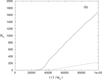
FIG. 6.: (a) Condensate fraction ($N_{0}/N$) as a function of time, in units of $\omega_{g}^{-1}$, for the case of $\gamma_{eff}=0.01\omega_{g}$, and $a=6$nm, and $m_{max}=60$ (solid) and $30$ (dashed); (b) Dynamics of $N_{0}$ for the same situation; (c) Evolution of the energy per particle for the same conditions.

We have also analyzed the case in which an already formed condensate is emptied via outcoupling, and continuously pumped via spontaneous emission from the thermal reservoir. In our simulations we just consider outcoupling from the condensate, although similar methods could be employed to simulate losses affecting the whole trap. We simulate without outcoupling the creation of a condensate as described above, for the case of $\gamma_{eff}=6.28\omega_{g}$ , and $m_{max}=10$. For the case of ⁵²Cr, and $2\gamma_{eg}=200$s^-1. This represents a quite large phase space density $6\times 10^{-3}$; however, we must again stress that the BRE allows to work with much larger $\gamma_{eg}$, and therefore with much lower phase space densities of the reservoir. At $t=350$ms (when $N_{0}\simeq 950$), we begin the outcoupling. We have analyzed different outcoupling rates $\gamma_{out}$ (Fig. 7), and monitored the population $N_{0}$ after $16$s. This allows us to find a critical threshold $\xi_{0}$ (for this case $1.14$) for the ratio $\xi=\gamma_{out}/\gamma_{eff}$. For $\xi>\xi_{0}$ the loading (“gain”) is faster than the outcoupling (“loss”), and the number of condensate atoms increases with time. For $\xi<\xi_{0}$, the number of particles decreases and stabilizes for a lower $N_{0}$. For $\xi\ll\xi_{0}$ no condensate can be kept.

FIG. 7.: Number of condensed particles after $16$s (after initially loading an empty $|g\rangle$ trap during $350$ms) for the case of $\omega=2\pi\times 1$kHz, $m_{max}=10$, $\gamma_{eff}=6.28\omega_{g}$, and different outcoupling rates $\gamma_{out}$.

FIG. 8.: Condensate population, averaged during $40$s for the case of $m_{max}=10$, $\gamma_{eff}=6.28\omega_{g}$, $\omega_{g}=2\pi\times 1$kHz, $\gamma_{out}=(1.17-f(t))\gamma_{eff}$, with $0<f(t)<0.05$ chosen randomly from an uniform distribution.

It turns out to be important to maintain the population as constant as possible, for the reasons that we clarify below, and therefore to work in the regime of $\xi=\xi_{0}$. It is however not an easy task, due to the stochastic nature of both, the collisions and the pumping mechanism. In order to stabilize the noise optimally, i.e. to preserve the population of the condensate as constant as possible it is useful to introduce a random temporal variation of the outcoupling rate. Fig. 8 shows the averaged distribution of population of the condensate during $40$ s of continuous outcoupling, for the case of an outcoupling rate $\gamma_{out}=(1.17-f(t))\gamma_{eff}$, with $0<f(t)<0.05$ chosen randomly from an uniform distribution, and the same conditions as in Fig. 7. The population of the condensate is maintained quasiconstant with an average value of $\langle N_{0}\rangle=940$, and a variance $(\langle N_{0}^{2}\rangle-\langle N_{0}\rangle^{2})^{1/2}=80$. During these $40$s, $3\times 10^{5}$ atoms are extracted from the condensate, with a rate of $7500$ atoms/s.

Let us briefly comment about the importance of keeping the population of the condensate as constant as possible. The mean–field interaction translates the variations of the condensate population into variations of the energy of the outcoupled atoms, being the variance of the energy related to the variance of the condensate density: $\sigma(E)=4\pi\hbar^{2}a\sigma(n_{0})/m$. Therefore, the narrower the population distribution of the condensate, the more ”monochromatic” will be the atom–laser source, and consequently the larger the coherence time will be [36]. Let us point out finally, that an additional way to control the fluctuations of the condensate population could be provided by monitoring the energy of the outcoupled atoms, which would inform about the variations of the condensate density. Such information could be used in a feedback loop to dynamically adapt the outcoupling rate to reduce the energy variance of the outcoupled atoms, and therefore increase their temporal coherence.

VII Conclusions

In this paper we have analyzed a possible mechanism which could allow the creation and continuous loading of a condensate from a thermal reservoir, by optical pumping. In order to achieve such loading mechanism, it is necessary to guarantee that the reabsorptions of the spontaneously emitted photons do not lead to undesired heating of the atoms in the trap. We have analyzed a particular scheme which allows to satisfy such condition. In this scheme an atom forms a three level $\Lambda$ system, in which one of the transitions decays much faster than the other one. By using quantum Master Equation techniques we have shown that the very small branching ratio between both transitions induces very large reduction of probability of the reabsorption processes which change the population in the lowest state of the slower transition. We have explained such effect by identifying the photon reabsorption as a process whose probability depends on the correlation between the reabsorption amplitudes at different times. Such correlation is rapidly destroyed by the fast decay into the other possible channel. The destruction of this correlation causes the desired effect, i.e. the reduction of the “bad” reabsorption processes, responsible for possible heating.

Once we have shown that the reabsorption has no significative effect on the system, we have analyzed the loading dynamics from a thermal reservoir, using Monte Carlo simulations, including the atom–atom collisions in the QBME formalism. We have analyzed the loading of an initially empty trap, demonstrating that the onset of the condensation appears after a finite time, which depends on the physical parameters of the system. The condensation appears due to the joint combination of thermalization via collisions, evaporative cooling due to the finite depth of the considered trap, and bosonic enhancement of the pumping process. We have also analyzed the continuous refilling of the condensate, once it has been formed, taking at the same time into account continuously outcoupling. We have shown that the refilling mechanism allows the compensation of the losses introduced by the outcoupling, and we have analyzed the best strategies to keep the condensate population quasiconstant, which is important in order to achieve a “monochromatic” atom laser output. In the paper we have only analyzed the outcoupling mechanism, but the same reasonings applies to possible condensate losses, produced by inelastic processes, such as three–body recombination, or collisions with the thermal atoms in the reservoir.

All our simulations and estimates have been done for Chromium atoms, and for the parameters of the experiment currently performed at the University of Stuttgart. It is however interesting to stress that the same scheme is general, and in particular can be applied for other atomic systems, such as Magnesium[37]. As a final remark, we would like to stress that the mechanism of avoiding the “bad” reabsorption processes, considered in this paper (i.e. regime of BRE) allows for faster pumping than other reabsorption remedies (such as Festina Lente, for instance), and therefore allows for more effective compensation of the condensate losses. It offers a novel and interesting perspective towards a continuously loaded atom laser.

We acknowledge support from Deutsche Forschungsgemeinschaft (SFB 407), from the EU through the TMR network ERBXTCT96-0002, and from ESF PESC Programm BEC2000+. We acknowledge fruitful discussions with W. Ertmer, E. Rasel, K. Sengstock, and M. Wilkens.

REFERENCES

- [1] S. Chu, Nobel Lecture, Rev. Mod. Phys. 70, 685 (1998), C. Cohen–Tannoudji, Nobel Lecture, ibid., 707; W. D. Phillips, Nobel Lecture, ibid., 721.
- [2] M. H. Anderson et al., Science 269, 198 (1995); K.B. Davis, M. O. Mewes, M. R. Andrews, N. J. van Drutten, D. S. Durfee, D. M. Kurn and W. Ketterle, Phys. Rev. Lett. 75, 3969 (1995); C. C. Bradley, C. A. Sackett, and R. G. Hulet, ibid. 78, 985 (1997).
- [3] Proceedings of the International School of Physics “Enrico Fermi”, Course CXL, eds. M. Inguscio, S. Stringari, and C. Wieman (IOS Press, Amsterdam 1999).
- [4] C. Raman, M. Köhl, R. Onofrio, D. S. Durfee, C. E. Kuklewicz, Z. Hadzibabic, and W. Ketterle, Phy. Rev. Lett. 83, 2502 (1999).
- [5] O. M. Moragò, S. A. Hopkins, J. Arlt, E. Hodby, G. Hechenblaikner, and C. J. Foot, Phys. Rev. Lett. 84, 2056 (2000).
- [6] M. R. Matthews, B. P. Anderson, P. C. Haljan, D. S. Hall, C. E. Wieman, and E. A. Cornell, Phys. Rev. Lett. 83, 2498 (1999).
- [7] K. W. Madison, F. Chevy, W. Wohlleben, and J. Dalibard, Phys. Rev. Lett. 84, 806 (2000).
- [8] J. Denschlag, J. E. Simsarian, D. L. Feder, Charles W. Clark, L. A. Collins, J. Cubizolles, L. Deng, E. W. Hagley, K. Helmerson, W. P. Reinhardt, S. L. Rolston, B. I. Schneider, and W. D. Phillips, Science 287, 97 (2000).
- [9] S. Burger, K. Bongs, S. Dettmer, W. Ertmer, K. Sengstock, A. Sanpera, G. V. Shlyapnikov, and M. Lewenstein, Phys. Rev. Lett. 83, 5198 (1999).
- [10] C.S. Adams, M. Sigel, J. Mlynek, Phys. Rep. 240, 145 (1994).
- [11] S. Inouye, T. Pfau, S. Gupta, A.P. Chikkatur, A. G rlitz, D. E. Pritchard, W. Ketterle, Nature 402, 641 (1999). M. Kozuma, Y. Suzuki, Y. Torii, T. Sugiura, T. Kuga, E. W. Hagley, L. Deng, Science 286, 2309 (1999).
- [12] K. Bongs, S. Burger, G. Birkl, K. Sengstock, W. Ertmer, K. Rza̧żewski, A. Sanpera, M. Lewenstein, Phys. Rev. Lett. 83, 3577 (1999).
- [13] L. Deng, E. W. Hagley, J. wen, M. Trippenbach, Y. Band, P. S. Julienne, J. E. Simsarian, K. Helmerson, S. L. Roston, and W. D. Phillips, Nature 398, 218 (1999).
- [14] M.-O. Mewes, M. R. Andrews, D. M. Kurn, D. S. Durfee, C. G. Townsend, and W. Ketterle, Phys. Rev. Lett. 78, 582 (1997).
- [15] M. R. Andrews, C. G. Townsend, H.-J. Miesner, D. S. Durfee, D. M. Kurn, and W. Ketterle, Science 275, 637 (1997).
- [16] I. Bloch, T. W. Hänsch, and T. Esslinger, Nature 403, 166 (2000).
- [17] S. Burger, K. Bongs, K. Sengstock and W. Ertmer, Proc. Int. Scholl of Quant. Elec., 27th Course, Erice, Italy (1999), in print Kluver Academic, Amsterdam, 2000.
- [18] E. W. Hagley, L. Deng, M. Kozuma, J. Wen, K. Helmerson, S. L. Rolston, and W. D. Phillips, Science 283, 1706-1709 (1999).
- [19] for a recent proposal E. Mandonnet, A. Minguzzi, R. Dum, I. Carusotto, Y. Castin, J. Dalibard, Euro. Phys. J. D (to be published); cond-mat/9909378 and references therein.
- [20] R. J. C. Spreeuw, T. Pfau, U. Janicke and M. Wilkens, Europhys. Lett. 32, 469 (1995); U. Janicke and M. Wilkens, Adv. At. Mol. Opt. Phys. 41, 261 (1999) and references therein .
- [21] M. Olshan’ii,Y. Castin, and J. Dalibard, Proc. 12th Int. Conf. on Laser Spectroscopy, M. Inguscio, M. Allegrini, and A. Lasso, Eds. (World Scientific, Singapour, 1996).
- [22] A. M. Smith and K. Burnett, J. Opt. Soc. Am. B 9, 1256 (1992).
- [23] T. Pfau, and J. Mlynek, OSA Trends in Optics and Photonics Series 7, 33 (1997).
- [24] Y. Castin, J. I. Cirac, and M. Lewenstein, Phys. Rev. Lett. 80, 5305 (1998).
- [25] U. Janicke and M. Wilkens, Europhys. Lett. 35, 561 (1996).
- [26] J. I. Cirac, M. Lewenstein, and P. Zoller, Europhys. Lett. 35, 647 (1996).
- [27] J. I. Cirac and M. Lewenstein, Phys. Rev. A 53, 2466 (1996).
- [28] C. Gardiner, Handbook of Stochastic Methods, Springer Verlag, 1985; C. W. Gardiner and P.Zoller, Quantum Noise, Springer-Verlag, 1999; Howard Carmichael, An Open Systems Approach to Quantum Optics, Springer-Verlag, 1993.
- [29] L. Santos and M. Lewenstein, Phys. Rev. A, 60, 3851 (1999).
- [30] C. W. Gardiner and P. Zoller, Phys, Rev. A 55, 2902 (1997)
- [31] D. Jaksch, C. W. Gardiner and P. Zoller, Phys. Rev. A 56, 575 (1997).
- [32] L. Santos and M. Lewenstein, Appl. Phys. B 69, 363 (1999).
- [33] M. Holland, J. Williams and J. Cooper, Phys. Rev. A 55, 3670 (1997).
- [34] The large–temperature approximation is assumed since it simplifies the numerical simulation. Although this approximation has certain physical consequences, we want to stress that similar effects as the ones discussed in this paper are not only possible for the case of lower temperatures, but should in principle allow for faster loading. In such a case, the Franck–Condon factors of the different transitions should be properly calculated (c.f. [20, 29]).
- [35] For a discussion in the case of Festina Lente regime see L. Santos, Z. Idziaszek, J. I. Cirac, and M. Lewenstein, in print in the Speccial Issue of J. Phys. B on “Coherent Matter Waves”, ed. K. Burnett (2000).
- [36] M. Holland, K. Burnett, C. Gardiner, J. I. Cirac, and P. Zoller, Phys. Rev. A 54, R1757 (1996).
- [37] The latter possibility is considered by the W. Ertmer/E. Rasel group at the University of Hannover.