620021 arXiv version with permission from EDP Sciences http://www.edpsciences.org/euro/ Foundations of quantum mechanics; measurement theory

A Kochen-Specker inequality

Abstract

By probabilistic means, the concept of contextuality is extended so that it can be used in non-ideal situations. An inequality is presented, which at least in principle enables a test to discard non-contextual hidden-variable models at low error rates, in the spirit of the Kochen-Specker theorem. Assuming that the errors are independent, an explicit error bound of 1.42% is derived, below which a Kochen-Specker contradiction occurs.

The description of quantum-mechanical processes by hidden variables is a subject being actively researched at present. The interest can be traced to topics where recent improvements in technology has made testing and using quantum processes possible. Research in this field is usually intended to provide insight into whether, how, and why quantum processes are different from classical processes. Here, the presentation will be restricted to the question whether there is a possibility of describing a certain quantum system using a non-contextual hidden-variable model or not. A non-contextual hidden-variable model would be a model where the result of a specific measurement does not depend on the context, i.e., what other measurements that are simultaneously performed on the system. It is already known that in the ideal case no non-contextual model exists. These results can be traced to the work of Gleason [1], but a conceptually simpler proofs was given by Kochen and Specker (KS) [2].

The original KS theorem concerns measurements on a quantum system consisting of a spin-1 particle. In the quantum description of this system, the operators associated with measurement of the spin components along orthogonal directions do not commute, i.e.,

$$\hat{S}_{\mathbf{x}},\hat{S}_{\mathbf{y}},\text{ and }\hat{S}_{\mathbf{z}}\text{ do not commute.}$$ (1)

however, the operators that are associated with measurement of the square of the spin components do commute, i.e.,

$$\hat{S}^{2}_{\mathbf{x}},\hat{S}^{2}_{\mathbf{y}},\text{ and }\hat{S}^{2}_{\mathbf{z}}\text{ commute.}$$ (2)

The latter operators (the squared ones) have the eigenvalues 0 and 1, and

$$\hat{S}^{2}_{\mathbf{x}}+\hat{S}^{2}_{\mathbf{y}}+\hat{S}^{2}_{\mathbf{z}}=2\mathbb{I}.$$ (3)

Thus, it is possible to simultaneously measure the square of the spin components along three orthogonal vectors, and two of the results will be 1 while the third will be 0. Only this quantum-mechanical property of the system will be used in what follows. A hidden-variable model of this system is now non-contextual if the result when measuring $\hat{S}^{2}_{\mathbf{x}}$ is independent of whether $\hat{S}^{2}_{\mathbf{y}}$ and $\hat{S}^{2}_{\mathbf{z}}$ are measured simultaneously or $\hat{S}^{2}_{\mathbf{y}^{\prime}}$ and $\hat{S}^{2}_{\mathbf{z}^{\prime}}$ are. That is, measurement along one direction should yield the same result irrespective of the other (commuting) measurements made, so that the result of a measurement does not depend on the context. The idea of the KS theorem is to choose a set of orthonormal triads so that assignment of 0/1 results to the corresponding measurements is impossible.

However, idealizations are needed in the KS theorem that are not usable in experimental situations. The most obvious idealization is that the measurement results are assumed to be without errors. Also, it is assumed that all measurements yield results (no missing detections). Further, a more subtle point is whether it is at all possible to align two measurement setups so that there is one common measurement, being made in different contexts (this question is raised by Meyer, Kent and Clifton (MKC) [3]). Lastly, it is often stated that to detect changes due to the context, we need to prepare several systems so that the hidden variables are identical. Here, a probabilistic analysis of the theorem will be provided, addressing these issues so that, at least in principle, an experimental test will be possible. But let us first look at the ideal case.

To describe the hidden-variable model, standard probability theory will be used, where the hidden variable $\lambda$ is a point in a probabilistic space $\Lambda$, and sets in this space (“events”) have a probability given by the probability measure $P$. The measurement results are described by random variables (RVs) $X_{i}(\lambda)$, which take their values in the value space $V=\{0,1\}$. To describe the measurement results, RVs are used so that formally the results are

$$\begin{pmatrix}X_{1}({\mathbf{x}},{\mathbf{y}},{\mathbf{z}},\lambda)\\ X_{2}({\mathbf{x}},{\mathbf{y}},{\mathbf{z}},\lambda)\\ X_{3}({\mathbf{x}},{\mathbf{y}},{\mathbf{z}},\lambda)\end{pmatrix},$$ (4)

which can take the results 0 or 1. The RV $X_{1}$ is associated with ${\mathbf{x}}$, $X_{2}$ with ${\mathbf{y}}$, and $X_{3}$ with ${\mathbf{z}}$; in a non-contextual hidden-variable model, $X_{1}$ would not depend on the arguments ${\mathbf{y}}$ and ${\mathbf{z}}$, for example. To shorten the notation, the following symmetries of the measurement results are assumed to hold (the proofs go through without the symmetry, but grow notably in size):

$$X_{1}({\mathbf{x}},{\mathbf{y}},{\mathbf{z}},\lambda)=X_{2}({\mathbf{z}},{\mathbf{x}},{\mathbf{y}},\lambda)=X_{3}({\mathbf{y}},{\mathbf{z}},{\mathbf{x}},\lambda).$$ (5)

In the analysis, we will use a set of pairwise interconnected triads using the notation

$$E=\left\{\begin{pmatrix}{\mathbf{e}}_{1}\\ {\mathbf{e}}_{2}\\ {\mathbf{e}}_{3}\end{pmatrix},\begin{pmatrix}{\mathbf{e}}_{1}\\ {\mathbf{e}}_{4}\\ {\mathbf{e}}_{5}\end{pmatrix},\cdots,\begin{pmatrix}{\mathbf{e}}_{n-2}\\ {\mathbf{e}}_{n-1}\\ {\mathbf{e}}_{n}\end{pmatrix}\right\}.$$ (6)

In this set there are $n$ vectors forming $N$ distinct orthogonal triads where some vectors are present in more than one triad, establishing in total $M$ connections by rotation around a vector. The KS theorem may now be stated.

Theorem 1: (Kochen-Specker) There exists a set of vector triads $E_{\text{KS}}$, so that the following two prerequisites cannot hold simultaneously for any $\lambda$

1. Non-contextuality. For any pair of triads in $E_{\text{KS}}$ related by a rotation around a vector, the result along that vector is not changed by the rotation. For example,

   $$X_{1}({\mathbf{x}},{\mathbf{y}},{\mathbf{z}},\lambda)=X_{1}({\mathbf{x}},{\mathbf{y}}^{\prime},{\mathbf{z}}^{\prime},\lambda).$$ (7)

2. Quantum-mechanical results. For any triad in $E_{\text{KS}}$, the sum of the results is two, i.e.,

   $$\sum_{i}X_{i}({\mathbf{x}},{\mathbf{y}},{\mathbf{z}},\lambda)=2.$$ (8)

A proof of the Kochen-Specker (KS) theorem is essentially a specification of $E_{\text{KS}}$, and a check that (i) and (ii) indeed cannot hold simultaneously. A full proof will not be provided here (the original $E_{\text{KS}}$ from [2] contains 117 vectors), but a simplified walk-through is highly useful in what follows. The proof is by contradiction; assume that Theorem 1 (i–ii) holds on $E_{\text{KS}}$ for some $\lambda$, and use (ii) to assign values to $X_{i}({\mathbf{e}}_{1},{\mathbf{e}}_{2},{\mathbf{e}}_{3},\lambda)$. Now, rotate using (i) to yield $X_{1}({\mathbf{e}}_{1},{\mathbf{e}}_{4},{\mathbf{e}}_{5},\lambda)$, and use (ii) to assign values to $X_{2}({\mathbf{e}}_{1},{\mathbf{e}}_{4},{\mathbf{e}}_{5},\lambda)$ and $X_{3}({\mathbf{e}}_{1},{\mathbf{e}}_{4},{\mathbf{e}}_{5},\lambda)$. Rotate again, and continue. The value for many RVs at later triads in the set will be determined by (i) and previous assignments, so there will be less choices as we continue. Now, when we arrive at the last triad in $E_{\text{KS}}$, all three values will already be fixed by (i) and previous assignments so that

$$\sum_{i}X_{i}({\mathbf{e}}_{n-2},{\mathbf{e}}_{n-1},{\mathbf{e}}_{n},\lambda)\neq 2,$$ (9)

in contradiction to (ii). This will occur whatever choices we make in our assignments (when we are free to make choices), which completes the proof of the KS theorem.

Let us now generalize this theorem to take into account the different kinds of non-ideal conditions occurring in experiment. The two first problems presented above is easiest to manage. Errors can be of two kinds: there can be (i) errors when changing context (e.g., a change in $X_{1}$ when changing $({\mathbf{y}},{\mathbf{z}})\to({\mathbf{y}}^{\prime},{\mathbf{z}}^{\prime})$) or (ii) errors in the sum. Missing results are also of two kinds: (i) when changing context or (ii) in one or more of the three $X_{i}$s so that the sum cannot be checked. These two can fairly easily be incorporated into a generalized theorem, by estimating the rate of errors. The question whether equal alignment in one direction is possible can be addressed as follows: consider a measurement device as depicted in fig. 1, presumably applied to a spin-1 system.

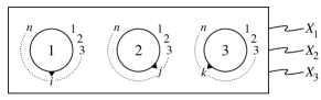
Figure 1: A Kochen-Specker experimental device. Inputs are the setting indices $(i,j,k)$, and outputs are $X_{m}$ taking the value 0 or 1, so that $\sum_{m}X_{m}=2$.

In fig. 1, the (macroscopic, distinct) settings on the inputs indicate which direction the measurements should be performed in. It is now entirely possible that e. g. the index-triple $(1,2,3)$ corresponds to the triad $({\mathbf{e}}_{1},{\mathbf{e}}_{2},{\mathbf{e}}_{3})^{T}$ while the index-triple $(1,4,5)$ corresponds to the triad $({\mathbf{e}}_{1}^{\prime},{\mathbf{e}}_{4},{\mathbf{e}}_{5})^{T}$, so that the first vector changes although the first index does not. This may be due to a non-ideal measurement device, or perhaps to an MKC effect. The effect on the results, however, is only a possible change in the result $X_{1}$ even though the first index has not changed, i.e., an error in (i) when changing the context. And errors of this type can be incorporated as indicated above.

Lastly, it is often said that to show contextuality in an experiment, it is necessary to prepare several systems so that the hidden variables are identical; this is to make a point-wise analysis (in $\Lambda$) of the condition (i). The below theorem is a statistical theorem that provides a global analysis on the whole sample set $\Lambda$, much in the same spirit as in [4], where this issue also is examined. The statement of Theorem 2 may seem slightly awkward; I have chosen to preserve the structure of Theorem 1 (note the similarities of (i-ii) in Theorems 1 and 2). A simpler statement will be provided in a later corollary.

Theorem 2: (Kochen-Specker inequality) Given a KS set $E_{\text{KS}}$ of $N$ vector triads with $M$ interconnections by rotation, if

$$M\delta+N\epsilon<1,$$ (10)

the following two bounds cannot hold simultaneously.

1. “Rotation” error bound. For any pair of triads in $E_{\text{KS}}$ related by a rotation around a vector, the set of $\lambda$s where the result along that vector is not changed by the rotation is large (has probability greater than $1-\delta$). For example,

   $$P\bigg{(}\Big{\{}\lambda:X_{1}({\mathbf{x}},{\mathbf{y}},{\mathbf{z}},\lambda)=X_{1}({\mathbf{x}},{\mathbf{y}}^{\prime},{\mathbf{z}}^{\prime},\lambda)\Big{\}}\bigg{)}\geq 1-\delta.$$ (11)

2. “Sum” error bound. For any triad in $E_{\text{KS}}$, the set of $\lambda$s where the sum of the results is two is large (has probability greater than $1-\epsilon$), i.e.,

   $$P\bigg{(}\Big{\{}\lambda:\sum_{i}X_{i}({\mathbf{x}},{\mathbf{y}},{\mathbf{z}},\lambda)=2\Big{\}}\bigg{)}\geq 1-\epsilon.$$ (12)

Proof: We have (using $\complement$ to denote complement)

$$P\bigg{(}\Big{\{}\lambda:X_{1}({\mathbf{x}},{\mathbf{y}},{\mathbf{z}},\lambda)=X_{1}({\mathbf{x}},{\mathbf{y}}^{\prime},{\mathbf{z}}^{\prime},\lambda)\Big{\}}^{\complement}\bigg{)}\leq\delta,$$ (13a)

$$P\bigg{(}\Big{\{}\lambda:\sum_{i}X_{i}({\mathbf{x}},{\mathbf{y}},{\mathbf{z}},\lambda)=2\Big{\}}^{\complement}\bigg{)}\leq\epsilon,$$ (13b)

so that,

$$P\bigg{(}\Big{(}\underset{M}{\bigcap}\Big{\{}\lambda:X_{1}({\mathbf{x}},{\mathbf{y}},{\mathbf{z}},\lambda)=X_{1}({\mathbf{x}},{\mathbf{y}}^{\prime},{\mathbf{z}}^{\prime},\lambda)\Big{\}}\Big{)}\bigcap\Big{(}\underset{N}{\bigcap}\Big{\{}\lambda:\sum_{i}X_{i}({\mathbf{x}},{\mathbf{y}},{\mathbf{z}},\lambda)=2\Big{\}}\Big{)}\bigg{)}$$

$$=1-P\bigg{(}\Big{(}\underset{M}{\bigcup}\Big{\{}\lambda:X_{1}({\mathbf{x}},{\mathbf{y}},{\mathbf{z}},\lambda)=X_{1}({\mathbf{x}},{\mathbf{y}}^{\prime},{\mathbf{z}}^{\prime},\lambda)\Big{\}}^{\complement}\Big{)}\bigcup\Big{(}\underset{N}{\bigcup}\Big{\{}\lambda:\sum_{i}X_{i}({\mathbf{x}},{\mathbf{y}},{\mathbf{z}},\lambda)=2\Big{\}}^{\complement}\Big{)}\bigg{)}$$

$$\geq 1-\sum_{M}P\Big{(}\Big{\{}\lambda:X_{1}({\mathbf{x}},{\mathbf{y}},{\mathbf{z}},\lambda)=X_{1}({\mathbf{x}},{\mathbf{y}}^{\prime},{\mathbf{z}}^{\prime},\lambda)\Big{\}}^{\complement}\Big{)}-\sum_{N}P\Big{(}\Big{\{}\lambda:\sum_{i}X_{i}({\mathbf{x}},{\mathbf{y}},{\mathbf{z}},\lambda)=2\Big{\}}^{\complement}\Big{)}$$

$$\geq 1-M\delta-N\epsilon.$$ (14)

The intersection set in the first probability at the top is empty by Theorem 1, i.e., the probability has to be zero. Thus, when the last expression is strictly positive (when $M\delta+N\epsilon<1$), we have a contradiction. $\square$

Note the explicit use of complement to take care of situations when there is no measurement result. Thus, in Theorem 2, one need not assume that the detected statistics correspond to that of the whole ensemble (this is commonly known as the “no-enhancement assumption”). Unfortunately inefficient detector devices would contribute no-detection events to both the error rates $\delta$ and $\epsilon$, which puts a rather high demand on experimental equipment. While the no-enhancement assumption can be used in inefficient setups, this may weaken the statement (cf. a similar argument for the GHZ paradox [5]). Also, as we shall see below, even when using the no-enhancement assumption here, the demands on experimental equipment are high.

The error rate $\epsilon$ is the probability of getting an error in the sum (both non-detections and the wrong sum are errors here), not the probability of getting an error in an individual result, and this makes it easy to extract $\epsilon$ from experimental data. Unfortunately, the errors that arise in rotation are not available in the experimental data so it is not possible to estimate the size of $\delta$ (note that it is not even meaningful to discuss $\delta$ in quantum mechanics). It is possible to use $\epsilon$ to obtain a bound for $\delta$:

Corollary 3 (Kochen-Specker inequality) Given a KS set of $N$ vector triads $E_{\text{KS}}$ with $M$ interconnections by rotation, if Theorem 2 (i-ii) hold, then

$$\delta\geq\frac{1-N\epsilon}{M}.$$ (15)

As can be seen above, a small $E_{\text{KS}}$ set (small $N$ and $M$) is better, yielding a higher bound for $\delta$ for a given $\epsilon$. In an inexact experiment yielding a large $\epsilon$, the bound in Corollary 3 will be low. Being an inexact experiment, one expects the error rate $\delta$ to be large also, thus not violating Corollary 3; changes in a result due to the context may be attributed to (normal) measurement errors. A model for this inexact experiment can then be said to be “probabilistically non-contextual”. In a better experiment yielding a low $\epsilon$, the bound in Corollary 3 is higher. But here one expects $\delta$ to be low as well, in violation of Corollary 3. In a hidden-variable model of this experiment, the changes in a result due to the context occur at an unexpectedly high rate which cannot be attributed to measurement errors, and a model of this type can be said to be “probabilistically contextual”.

A small further discussion of the MKC [3] constructions is appropriate here (see also [6]). The argument is that due to the finite precision of measurement device orientations, we may only get measurement results from a (dense) subset of vectors on the unit sphere. One of the constructions then proceeds to devise a dense subset of vectors on the unit sphere such that Theorem 1 cannot be applied. Results may now be assigned to each measurement following the quantum rule (ii) on the whole dense subset, without any contradiction (the other constructions are similar). Now, the MKC models are argued to be non-contextual in the sense that only the vector along which the measurement is made is needed to fix the value of the RV. An important observation is that in the MKC models there is only one context in which each measurement is contained; mathematically in (i), the set $\{\lambda:X_{1}({\mathbf{x}},{\mathbf{y}},{\mathbf{z}},\lambda)=X_{1}({\mathbf{x}},{\mathbf{y}}^{\prime},{\mathbf{z}}^{\prime},\lambda)\}$ is not well-defined; there are no distinct triads $({\mathbf{x}},{\mathbf{y}},{\mathbf{z}})$, $({\mathbf{x}},{\mathbf{y}}^{\prime},{\mathbf{z}}^{\prime})$ that can be inserted as arguments. Therefore, it can be argued that the question of (non-)contextuality is void; an MKC model is neither contextual nor non-contextual. Also note that Theorem 2 applies to any measurement device like that in fig. 1. Thus, even if the discussion can be continued as to whether contextuality is a valid concept for the MKC models at an internal level, one is forced to conclude that a hidden-variable model (including the measurement device) of a “good” experiment must be (probabilistically) contextual.

Until now, the present discussion has been limited to the original spin-1, 3-dimensional setting. However, there are higher-dimensional settings in which there are smaller $E_{\text{KS}}$, and Theorem 2 and Corollary 3 hold for these as well. All that is needed is a simple restatement of the prerequisites, i.e., in $d$ dimensions, the set $E$ consists of $N$ $d$-tuples with $M$ interconnections, and (i–ii) need additional vector entries as in $X_{i}({\mathbf{e}}_{1},\ldots,{\mathbf{e}}_{d},\lambda)$. Finally, in (ii) a more general specification of the results is that there should be one “zero” and the rest “ones”, so that the sum is $d-1$ (note that the labeling of the results differ in the literature).

Returning to the proof of Theorem 2, to obtain a general statement, there are no assumptions on independence of the errors, but it is possible to give a more quantitative bound for the error rate by introducing independence (for simplicity, using the no-enhancement assumption). Please note that there is no experimental check whether the assumption of independent errors holds or not. While the errors in the sum may be possible to check, it is not possible to extract what errors are present in the rotations or check for independence of those errors [7]. The below result is dimension-dependent; $d$ is the dimension.

Corollary 4 (KS inequality for independent errors): Assuming that the errors are independent at the rate $r$, both $\delta$ and $\epsilon$ are given by $r$. If Theorem 2 (i-ii) hold, then

$$M(2r-2r^{2})+N(1-(1-r)^{d}-(d-1)(1-r)^{d-2}r^{2})\geq 1.$$ (16)

Proof: In the case of independent errors at the rate $r$, the expressions for the probabilities in Theorem 2 (i) and (ii) are

$$\begin{split}P\bigg{(}\Big{\{}\lambda:X_{1}({\mathbf{x}},{\mathbf{y}},{\mathbf{z}},\lambda)=X_{1}({\mathbf{x}},{\mathbf{y}}^{\prime},{\mathbf{z}}^{\prime},\lambda)\Big{\}}\bigg{)}&=P(\text{no errors})+P(\text{flip on both }X_{1}\text{'s})\\ =(1-r)^{2}+r^{2}&=1-(2r-2r^{2}),\end{split}$$ (17a)

$$\begin{split}P\bigg{(}\Big{\{}\lambda:\sum_{i}X_{i}({\mathbf{x}},{\mathbf{y}},{\mathbf{z}},\lambda)=2\Big{\}}\bigg{)}&=P(\text{no errors})+P(\text{flip of the 0 and one 1})\\ =(1-r)^{d}+(d-1)(1-r)^{d-2}r^{2}&=1-(1-(1-r)^{d}+(d-1)(1-r)^{d-2}r^{2}).\end{split}$$ (17b)

The probabilities of these sets are not independent, so from this point on we cannot use independence, but the result follows easily from Theorem 2. $\square$

An expression of the form $r\geq f(N,M,d)$ can now be derived from Corollary 4, but this complicated expression is not central to the present paper. Again, to obtain a contradiction for high error rates $r$, a small $E_{\text{KS}}$ set is needed (small $N$ and $M$). It is now only a matter of looking at the various $E_{\text{KS}}$ available in the literature to determine $N$ and $M$, however, some care should be taken when doing this.

For example, the set presented in [8] contains 33 vectors forming 16 distinct triads. Unfortunately, some rotations used in the proof chain are not between two of these 16 triads; in some cases a rotation goes from one of the 16 triads to a pair of vectors (where the third vector needed to form a triad is not in the set), and a subsequent rotation returns us to another of the 16 triads. On these pairs, a modified result rule is used; there cannot be more than one “zero” in such a pair (see [8] Section 7-3 or [9] Section 3.2). Translating to the notation used here, an extra vector needs to be added in this case, and in the proof-chain in [8] Table 7-1, 8 extra vectors are needed; for symmetry reasons the total number of added vectors is 24, yielding $n=57$ and $N=40$ (note that these additional vectors are not needed to yield the KS contradiction if the modified result rule is used). Some care is also needed to determine $M$ from the extended set, and for the set in [8] this yields a total of $M=96$ rotations.

To conclude, for any hidden-variable model we have a bound on the rate $\delta$ of changes arising in rotation:

$$\delta\geq\frac{1-N\epsilon}{M}.$$ (18)

Here, $N$ is the number of triads in $E_{\text{KS}}$, $M$ is the number of connections within $E_{\text{KS}}$, and $\epsilon$ is the error rate in the sum. A proof using few triads with few connections yields a more restrictive bound. An inexact measurement producing a large $\epsilon$ leads one to expect a large $\delta$, which is in accordance with the inequality. A better experiment yielding a small $\epsilon$ leads one to expect a small $\delta$, which is not possible; any hidden-variable description of that physical system will have to be probabilistically contextual (i.e., yield a larger rate of changes in rotation than one would expect).

The above reasoning is qualitative, but if the assumption of independent errors is used, an explicit bound can be determined for the error rate $r$, and in the below table are a few examples (the $n$ column sometimes contains two numbers; the number in the parentheses pertains to the original set and the other to the extended set [13]).

The $r$ column contains the highest value for which a contradiction to (probabilistic) contextuality occurs. Obviously, a small KS set is better than a large one, yielding a contradiction at a higher $r$. Somewhat unexpectedly, Schütte’s 33-vector set is more economical in this sense than Kochen and Conway’s 31-vector set. In the above table we can see that there is a contradiction for the $E_{\text{KS}}$ from [12] as soon as $r<1.42\%$.

While writing this paper, the author learned from C. Simon that a similar approach was in preparation by him, Č. Brukner, and A. Zeilinger [14]. It should be noted that in that paper, $\delta$ is implicitly assumed to be zero.

The author would like to thank A. Kent for discussions. This work was partially supported by the QIT Programme in the European Science Foundation.

References

- [1] A. M. Gleason, J. Math. Mech. 6, 885, (1957).
- [2] S. Kochen and E. P. Specker, J. Math. Mech. 17, 59 (1967).
- [3] D. Meyer, Phys. Rev. Lett. 83, 3751 (1999); A. Kent, Phys. Rev. Lett. 83 3755 (1999); R. Clifton and A. Kent, Proc. R. Soc. Lond. A 456 2101 (2000).
- [4] A. Cabello, G. García-Alcaine, Phys. Rev. Lett. 80, 1797 (1998); C. Simon, M. Żukowski, H. Weinfurter and A. Zeilinger, Phys. Rev. Lett. 85, 1783 (2000).
- [5] D. M. Greenberger, M. Horne, A. Shimony, and A. Zeilinger, Am. J. Phys. 58, 1131 (1990); N. D. Mermin, Phys. Rev. Lett. 65, 1838 (1990); J.-Å. Larsson, Phys. Rev. A 57, R3145 (1998); J.-Å. Larsson, Phys. Rev. A 59, 4801 (1999).
- [6] H. Havlicek, G. Krenn, J. Summhammer, and K. Svozil, J. Phys. A 34, 3071 (2001); A. Cabello, http//arxiv.org/abs/quant-ph/9911024; N. D. Mermin, http//arxiv.org/abs/quant-ph/9912081; D. M. Appleby, http//arxiv.org/abs/quant-ph/0005010 and http//arxiv.org/abs/quant-ph/0005056.
- [7] A discussion of the assumption of independent errors is appropriate here, but such a discussion cannot be fit into this limited space.
- [8] A. Peres, J. Phys. A 24, L175 (1991); A. Peres, Quantum Theory: Concepts and Methods, Ch. 7 (Kluwer, Dordrecht, 1993).
- [9] J. Bub, Interpreting the Quantum World, Ch. 3 (Cambridge University Press, Cambridge, 1997).
- [10] M. Kernaghan and A. Peres, Phys. Lett. A 198, 1 (1995).
- [11] M. Kernaghan, J. Phys. A, 27, L829 (1994).
- [12] A. Cabello, J. M. Estebaranz, and G. García-Alcaine, Phys. Lett. A 212, 183 (1996); ibid. 218, 115 (1996).
- [13] It is possible in the cases when an extended set is needed, that an analysis more adapted to the structure of the original set yields a contradiction at a somewhat higher . Please also note that the observation by Clifton reported in [9, 12] that some vectors can be left out in [11, 12] is similar to pruning the extra vectors in the extension of e.g. Peres’s set [8].
- [14] C. Simon, Č. Brukner, and A. Zeilinger, Phys. Rev. Lett. 86, 4427 (2001).