Negative phase time for Scattering at Quantum Wells:
A Microwave Analogy Experiment

Abstract

If a quantum mechanical particle is scattered by a potential well, the wave function of the particle can propagate with negative phase time. Due to the analogy of the Schrödinger and the Helmholtz equation this phenomenon is expected to be observable for electromagnetic wave propagation. Experimental data of electromagnetic wells realized by wave guides filled with different dielectrics confirm this conjecture now.

The propagation of a wave packet is determined by the dispersion relation of the medium. E.g. in vacuum a plane wave propagates with a constant amplitude and a phase shift proportional to frequency. In the case of tunnelling through a barrier, the constant phase leads to propagation speeds faster than light, calculated by tunnel_theo and measured for microwaves, single photons and infrared light tunnel_exp1 ; tunnel_exp2 ; tunnel_exp3 . In the contrary case of particles scattered by a potential well instead of a barrier, Li and Wang predicted a non–evanescent propagation but also with negative phase shifts wang . We present here an experimental simulation of the quantum well by a microwave set–up performing the analogy between the Schrödinger and the Helmholtz equation.

Applying the stationary phase approximation, the peak value of a quantum mechanical wave packet with a mean impulse $p_{0}=\hbar k_{0}$ propagates with the group velocity $v_{\rm gr}=d\omega/dk|_{k_{0}}$. This relationship can also be described in terms of classical mechanics by $v_{\rm gr}=\frac{x}{\frac{d}{d\omega}kx}=\frac{x}{\tau}$, where particles traverse the distance $x$ in the time $\tau$. The term $kx=\varphi$ describes the change of phase for the considered distance, $\frac{d}{d\omega}\,\varphi=\tau_{\varphi}$ is the time necessary for the propagation, called phase time tunnel_theo .

Potential scattering at quantum wells

In order to analyze a particle scattered by a potential well, the Schrödinger equation must be solved for a potential as sketched in Fig. 1 (left). However, the analogy between the Schrödinger and the Helmholtz equation (1) allows to examine the same process in an experiment with electromagnetic waves, too.

$$\left[\frac{d^{2}}{dx^{2}}+\frac{2m}{\hbar^{2}}\left(E-V(x)\right)\right]\psi(x)=0\>,\quad\left[\frac{d^{2}}{dx^{2}}+\frac{1}{v^{2}}\left(\omega^{2}\!-\omega_{c}^{2}(x)\right)\right]\phi(x)=0$$ (1)

In contrast to quantum mechanics, the phase and the absolute value of the transmitted electromagnetic wave are measurable. Identical boundary conditions for the electromagnetic field $\phi$ (representing the E or H field) and the wave function $\psi$ lead to an analogous solution of the propagation problem hanna .

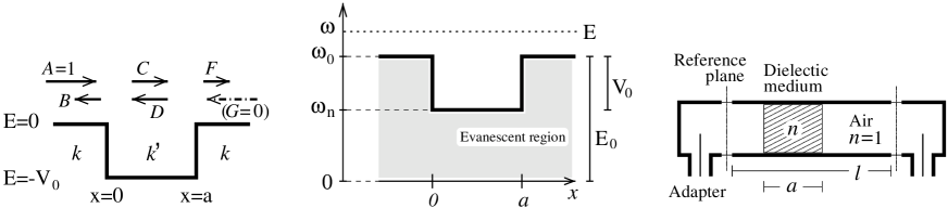
Figure 1: Energy levels of the quantum well, coefficients and wave numbers of the wave function (left); microwave analogy using wave guide sections with different cut–off frequencies $\omega_{0}$, $\omega_{n}$ (center); and the experimental set–up (right): a wave guide of fixed length $l$ is connected to a network analyzer by coaxial adaptors. It partially contains a dielectric medium of refractive index $n$, which represents the quantum well.

The energy level $V(x)$ of the quantum well can be constructed in a microwave experiment by wave guide sections with different cut–off frequencies $\omega_{c}(x)$, see Fig. 1 (center). Applying the analogy, the energy baseline of the well is shifted by a constant value $E_{0}=\hbar\omega_{0}$, which corresponds with the cut–off frequency $\omega_{0}$ of the first wave guide section. Using the following Ansatz for the wave function, see Fig. 1 (left):

$$\begin{array}[]{lll}&A\,e^{ikx}+B\,e^{-ikx}\>,&x\leq 0\\ \psi(x)=&C\,e^{ik^{\prime}\!x}+D\,e^{-ik^{\prime}\!x}\>,&0<x<a\\ &F\,e^{ik(x\!-\!a)}+G\,e^{-ik(x\!-\!a)}\>,&a\leq x\end{array}$$ (2)

This leads for energies $E>E_{0}$ to a wave propagation with the real wave numbers

$$k=\frac{1}{\hbar}\sqrt{2m(E-E_{0})}\quad{\rm and}\quad k^{\prime}=\frac{1}{\hbar}\sqrt{2m(E+V_{0}-E_{0})}\;.$$ (3)

Boundary conditions for the wave functions and their first derivatives at $x=0$ and $x=a$ determine the unknown coefficients $A$, $B$, $\ldots$ $G$ of (2), see merzbacher . Our definition of $\psi$ for $x\geq a$ implies, that the complete phase shift inside the well occurs only in the coefficients $F$ and $G$. Assuming an incident wave at $x=0$, we set $A=1$ and $G=0$ and find

$$F=\left[\cos k^{\prime}a-\frac{i}{2}\!\left(\!\frac{k^{\prime}}{k}\!+\!\frac{k}{k^{\prime}}\!\right)\!\sin k^{\prime}a\right]^{-1}.$$ (4)

Then, the complete phase shift of the transmitted wave at $x=a$ becomes

$$\varphi=\arg(F)=\arctan\!\left(\frac{1}{2}\!\left(\!\frac{k^{\prime}}{k}\!+\!\frac{k}{k^{\prime}}\!\right)\tan k^{\prime}a\right).$$ (5)

This formula is valid for both quantum mechanical and also electromagnetic wells, while the phase time $\tau_{\varphi}=\frac{d\varphi}{d\omega}=\frac{d\varphi}{dk}\frac{dk}{d\omega}$ depends on the dispersion relation $k(w)$ of the well in question.

Electromagnetic scattering in wave guides

Inside the wave guide the wave numbers obey the dispersion relations

$$k(\omega)=\frac{1}{c}\sqrt{\omega^{2}\!-\!\omega_{0}^{2}}\>,\quad k^{\prime}(\omega)=\frac{n}{c}\sqrt{\omega^{2}\!-\!\omega_{n}^{2}}\>,$$ (6)

where $c/n=v$ is the phase velocity in the medium. In the experimental set–up a rectangular wave guide of length $l=250$ mm is used, which is partially filled by a dielectric medium of refractive index $n$, Fig. 1 (right). The cut–off frequencies of the empty and the filled wave guide sections are $\omega_{0}=\pi c/b$ and $\omega_{n}=\pi c/nb$ respectively, where $b$ is the width of the wave guide. The used X–band wave guide ($b=22.86$ mm) filled with Teflon ($n=\sqrt{2.05}$) has the cut–off frequencies $f_{0}=\omega_{0}/2\pi=6.56$ GHz and $f_{n}=4.58$ GHz. Thus, the energy levels of the quantum well correspond to $E_{0}=\hbar\omega_{0}=27.1~{}\mu$eV, $V_{0}=\hbar(\omega_{0}\!-\!\omega_{n})=8.2~{}\mu$eV. The phase time $\tau_{\varphi}$, which describes the propagation of the maximum of a wave packet in the stationary phase approximation, is

$$\tau_{\varphi}=\frac{d\varphi}{d\omega}=\frac{a\,\omega}{c^{2}k}\frac{2n^{2}k^{2}(k^{\prime 2}\!\!+\!k^{2})-(k^{\prime 2}\!\!-\!k^{2})\,k^{\prime 2}_{0}\sin(2k^{\prime}a)/k^{\prime}a}{4k^{2}k^{\prime 2}+\left(k^{\prime 2}\!\!-\!k^{2}\right)^{2}\sin^{2}\!k^{\prime}a}$$ (7)

with constant $k^{\prime 2}_{0}=k^{\prime 2}\!\!-\!n^{2}k^{2}$. The high frequency limit of (7) for $k$, $k^{\prime}\to\infty$ is $\tau_{\varphi}=a\frac{\omega}{k}\frac{n^{2}}{c^{2}}$. With the phase velocity $v_{\rm ph}=w/k$ and the group velocity $v_{\rm gr}=a/\tau_{\varphi}$, Eq. (7) results in the well known relationship $v_{\rm gr}v_{\rm ph}=(c/n)^{2}$ for wave guides filled with a dielectric medium.

In Fig. 2 we plotted regions of negative phase time depending on the well width $a$ and the frequency $f$ using Eq. (7). The frequency range was chosen from the cut–off frequency of the empty wave guide $6.56$ up to $6.9~{}$GHz.

Figure 2: Regions of negative phase time $\tau_{\varphi}$ in seconds in a Teflon well according to Eq. (7): depending on frequency $f$ and well width $a$, negative phase times between 0 and -1 ns occur inside the marked regions. At the left side the diagram starts with the cut–off frequency of the unfilled wave guide $6.56$ GHz. Below this frequency value only evanescent modes can propagate through the wave guide. Only certain widths $a$ yield negative phase times. The longer the well, the smaller the frequency band in which negative phase times appear. The region of negative phase time in the vicinity of $a=0$ outreaches until approximately $7.6~{}$GHz.

Measurement at Teflon wells

To verify the predictions we filled tight–fitting pieces of Teflon into the wave guide. Some widths of the pieces fulfilled the condition for negative phase time laying inside the marked regions, while other pieces should not show negative phase times because their widths lay in between.

For each piece of Teflon, the scattering parameter $S_{21}$ for the transmission of the partially filled wave guide, which is defined as ratio of the transmitted to the incident wave, was determined in the frequency domain. The measurements were performed by a network–analyzer HP-8510, which allows an asymptotic measurement by eliminating undesired influences of the electrical connections by a calibration to two reference planes, Fig. 1 (right). The measured transmission $S_{21}$ has to be corrected by a factor describing the change of phase inside the unfilled wave guide sections of total length $l-a$:

$$F=S_{21}\cdot e^{-ik(l-a)}$$ (8)

With this operation, the reference planes in Fig. 1 (right) are shifted to the surfaces of the Teflon block. We used the measured transmission function of the unfilled wave guide $S^{\rm ref}_{21}$ as a reference. Thus, the total phase shift inside the medium, which should comply with (5), is obtained from the measured data by

$$\varphi={\rm arg}\left(S_{21}\right)-(l\!-\!a)\cdot{\rm arg}\!\left(S^{\rm ref}_{21}\right).$$ (9)

Figure 3 shows $|F|^{2}$ and the phase $\varphi$ of $F$ for microwave transmission as a function of frequency across the well for different widths $a$. For $a=38.7,62.6$ and $82.3$ mm the phase increases with increasing frequency, while for $a=4.0,27.0,47.5$ and $71.1$ mm the phase decreases near the cut–off frequency.

Figure 3: Absolute value $|F|^{2}$ and phase $\varphi$ of the transmission coefficient $F$ vs frequency for different widths of Teflon pieces. The absolute values are attenuated due to reflections at the discontinuities $x=0$, $a$ and by cut–off effects. For some widths ($a=4.0,27.0,47.5$ and $71.1$ mm) the phase $\varphi$ falls with increasing frequency. Thin lines represent the theoretical phase progression (5). To achieve a clear representation, the phase curves are arranged in ascending order of the well widths.

The phase time $\tau_{\varphi}=(2\pi)^{-1}d\varphi/df$ was calculated from the measured data by numerical derivation. Figure 4 presents the results for the phase time for transmission of the different Teflon pieces. For the wells widths $a=4.0,27.0,47.5$ and $71.1$ mm negative phase times appear, while the other wells show the normal behavior of a positive phase progression. The frequency intervals with negative phase times are in a fair agreement with the predicted intervals in Fig. 2.

Figure 4: Phase time $\tau_{\varphi}$ obtained from numerical derivation of the measured phase data of Fig. 3 and theoretical phase times (thin lines) calculated by (7). The curves for the well widths $a=4.0,27.0,47.5$, and $71.1$ mm show negative phase times at frequencies near the cut–off frequency of the unfilled wave guide. The non–vanishing resistance of real wave guide walls, especially near the cut–off frequency, may be in charge of the experimental deviations from the theoretical results.

Measurement at Perspex wells

To add further credibility to the measured negative phase times we modified the well depth $V_{0}$ by using Perspex as an alternative dielectric medium with $n=1.6$, $f_{n}=4.10$ GHz and $V_{0}=10.2~{}\mu$eV. According to Eq. (7), negative phase times are expected now for smaller well widths but for broader frequency bands, Fig. 5. Measurements are performed from 6.6 to 8.0 GHz and for well widths $a=6$, 18, and 24 mm, the wells $a=6$ and $24$ mm should show negative phase times. The measured phase progression in Fig. 6 (left) and the deduced phase times (right) are also in a good agreement with the theoretical predictions for the Perspex wells (thin lines). Although the well width $a=18$ mm lay close to a region of negative phase time, the measured phase progression of the well is clearly positive. This demonstrates how accurately the appearance of negative phase time depends on the width of the potential well.

Figure 5: Regions of negative phase time $\tau_{\varphi}$ in seconds for wells made of Perspex according to Eq. (7). The measurements were performed for the frequency interval between 6.6 and 8.0 GHz and for the well widths $a=6$, 18, and 24 mm. The wells $a=6$ and $24$ mm fulfil the condition for negative phase time.

Figure 6: Measured phase (left) and deduced phase time (right) for the Perspex wells. The phase progression is negative up to 7.1 GHz for the well $a=6$ mm and up to 6.7 GHz for $a=24$ mm. The oscillations around the theoretical curves (thin lines) may be caused by an impedance mismatch between the wave guide and the connectors. The well width $a=18$ mm lays outside the marked regions of Fig. 5, here the phase shows a normal positive progression.

Conclusions

The analogy between quantum mechanical and electromagnetic scattering has been investigated with microwaves. Theoretical studies wang predicted negative phase times for certain well widths if the energy of an incident particle is less than half the well depth. Actually, our measurements at two different well depths show the predicted negative phase times. For the first time, we demonstrate the effect of negative phase time for potential wells in a microwave analogy experiment.

Acknowledgements

We are grateful to C.-F. Li and Q. Wang for providing their theoretical study prior to publication, and P. Mittelstaedt for discussions on theory of quantum mechanical scattering.

References

- (1) Hartman, Th., J. Appl. Phys. 33 (1962) 3422
- (2) Enders, A., and Nimtz, G., J. Phys. I, France, 2 (1992) 1693
- (3) Steinberg, A., Kwiat, P., and Chiao, R., Phys. Rev. Letter 71 (1993) 708
- (4) Spielmann, Ch., Szipöcs, R., Stingle, A., and Krausz, F., Phys. Rev. Letter 73 (1994) 2308
- (5) Li, C.-F., and Wang, Q., submitted to Phys. Let. A
- (6) Brodowsky, H.M., Heitmann, W., and Nimtz, G., Phys. Let. A 222 (1996) 125
- (7) Merzbacher, E., Quantum Mechanics, 2nd ed., John Wiley & Sons, New York (1970)