New hydrogen-like potentials

Abstract

Using the modified factorization method employed in [5], we construct a new class of radial potentials whose spectrum for $l=0$ coincides exactly with that of the hydrogen atom. A limiting case of our family coincides with the potentials previously derived by Abraham and Moses [6].

1 Introduction.

In almost all exactly soluble spectral problems of the energy operator, the possibility of obtaining an exact expression for the energy levels and the corresponding eigenstates stems from the group theoretical symmetries which lead to the algebraic factorization method [1]-[3]. This method, until quite recently, appeared to have been fully explored. Yet, from time to time, some new potential arises for which the factorization method can be applied in a new way [4]. Recently, a variant of the factorization method proposed by Mielnik [5] has permitted a description of a new class of potentials whose spectra are identical to those of the harmonic oscillator [6]-[8]. Below we apply this method to show that there is a one-parameter class of radial potentials, different from a Coulomb field for which the sequence of energy eigenvalues for $l=0$ is exactly as for the hydrogen atom.

2 Hydrogen potential: standard and generalized factorizations.

As is well known, the hydrogen atom eigenproblem:

$$\left[-\frac{\hbar^{2}}{2m}\nabla^{2}-\frac{e^{2}}{r}\right]\psi({\bf r})=E\psi({\bf r}),$$ (2.1)

which, after the separation of the angular variables $\psi({\bf r})=Y(\theta,\varphi)R(r)$ leads to a sequence of radial problems:

$$\frac{1}{r}\left[-\frac{d^{2}}{dr^{2}}+\frac{l(l+1)}{r^{2}}-\frac{2}{r}\right]rR=\lambda R,$$ (2.2)

where $l=0,1,2,\dots$ labels the angular momentum eigenvalues, $r$ is a new dimensionless radial coordinate, and the functions $R=\{R(r)\}\ (0\leq r<+\infty)$ form a Hilbert space ${\cal H}_{r}$ with the scalar product defined by: $(R,R^{\prime})=4\pi\int_{0}^{+\infty}\overline{R(r)}R^{\prime}(r)r^{2}dr$. It is also well known that the radial Hamiltonians

$$H_{l}=\frac{1}{r}\left[-\frac{d^{2}}{dr^{2}}+\frac{l(l+1)}{r^{2}}-\frac{2}{r}\right]r$$ (2.3)

admit a sequence of ‘factorized forms’ which allows us to find very simply the energy levels [1]. These forms are

$$H_{l}=a_{l}^{+}a_{l}-\frac{1}{l^{2}}$$ (2.4)

$$H_{l}=a_{l+1}a_{l+1}^{+}-\frac{1}{(l+1)^{2}}$$ (2.5)

where

$$a_{l}=\frac{1}{r}\left[\frac{d}{dr}+\frac{l}{r}-\frac{1}{l}\right]r,$$ (2.6)

$$a_{l}^{+}=\frac{1}{r}\left[-\frac{d}{dr}+\frac{l}{r}-\frac{1}{l}\right]r.$$ (2.7)

Now, following the method in [5], we would like to ask two questions. Is this representation unique? Are $a_{l}$ and $a_{l}^{+}$ the only first-order differential operators for which (2.4)-(2.5) hold? It turns out that the answer is negative. Put:

$$A_{l}=\frac{1}{r}\left[\frac{d}{dr}+\beta_{l}(r)\right]r$$ (2.8)

$$A_{l}^{+}=\frac{1}{r}\left[-\frac{d}{dr}+\beta_{l}(r)\right]r$$ (2.9)

and demand that the formula analogous to (2.4) should be again valid:

$$A_{l}^{+}A_{l}=H_{l}+\frac{1}{l^{2}}.$$ (2.10)

This leads to

$$-\beta_{l}^{\prime}(r)+\beta_{l}^{2}(r)=\frac{l(l+1)}{r^{2}}-\frac{2}{r}+\frac{1}{l^{2}}.$$ (2.11)

Taking into account that we already have one particular solution, $\beta_{l}=(l/r)-(1/l)$ the general solution of (2.11) can be easily obtained. Denote

$$\beta_{l}=\frac{l}{r}-\frac{1}{l}+\phi_{l}(r).$$ (2.12)

Then

$$-\phi_{l}^{\prime}+\frac{2l}{r}\phi_{l}-\frac{2}{l}\phi_{l}+\phi_{l}^{2}=0.$$ (2.13)

After introducing a new function, $X_{l}=1/\phi_{l}$, we obtain:

$$X_{l}^{\prime}+\frac{2l}{r}X_{l}-\frac{2}{l}X_{l}+1=0$$ (2.14)

with the general solution

$$X_{l}=\left(\gamma_{l}-\int_{0}^{r}y^{2l}e^{-2y/l}dy\right)r^{-2l}e^{2r/l};\quad\gamma_{l}\in R$$ (2.15)

and, therefore,

$$\beta_{l}(r)=\frac{l}{r}-\frac{1}{l}+\frac{r^{2l}e^{-2r/l}}{\gamma_{l}-\int_{0}^{r}y^{2l}e^{-2y/l}dy}.$$ (2.16)

The commutator of the new operators $A_{l}$ and $A_{l}^{+}$ is not a number:

$$[A_{l},A_{l}^{+}]=2\beta_{l}^{\prime}(r).$$ (2.17)

Thus, we can apply the factorization method in a new way.

Taking the product $A_{l}A_{l}^{+}$, instead of $A_{l}^{+}A_{l}$ in (2.10), one has

$$A_{l}A_{l}^{+}=A_{l}^{+}A_{l}+[A_{l},A_{l}^{+}]=H_{l}+\frac{1}{l^{2}}+2\beta_{l}^{\prime}(r)=\tilde{H}_{l-1}+\frac{1}{l^{2}}$$ (2.18)

where $\tilde{H}_{l-1}$ is a new Hamiltonian:

$$\tilde{H}_{l-1}=H_{l}+2\beta_{l}^{\prime}(r)=\frac{1}{r}\left[-\frac{d^{2}}{dr^{2}}+\tilde{V}_{l-1}(r)\right]r,$$ (2.19)

with

$$\tilde{V}_{l-1}(r)=-\frac{2}{r}+\frac{l(l-1)}{r}+\frac{d}{dr}\left[\frac{2r^{2l}e^{-2r/l}}{\gamma_{l}-\int_{0}^{r}y^{2l}e^{-2y/l}dy}\right],\ l=1,2,3,\dots$$ (2.20)

If

$$\gamma_{l}>(2l)!\left(\frac{l}{2}\right)^{2l+1}$$

or $\gamma_{l}<0$ for a fixed $l$, the third term has no singularities. Furthermore, $\tilde{V}_{l-1}(r)\rightarrow 0$ as $r\rightarrow\infty$, and so we obtain a one-parameter family of new self-adjoint Hamiltonians. To find the spectra of $\tilde{H}_{l-1}$ note that:

$$\tilde{H}_{l-1}A_{l}=\left(A_{l}A_{l}^{+}-\frac{1}{l^{2}}\right)A_{l}=A_{l}\left(A_{l}^{+}A_{l}-\frac{1}{l^{2}}\right)=A_{l}H_{l}.$$ (2.21)

This implies that if $\{R_{nl}\}$ are eigenvectors of $H_{l}$ with eigenvalues $\lambda_{n}$, $\{A_{l}R_{nl}\}$ are eigenfunctions of $\tilde{H}_{l-1}$ with the same eigenvalues. Furthermore

$$A_{l}R_{nl}=a_{l}R_{nl}+\frac{r^{2l}e^{-2r/l}}{\gamma_{l}-\int_{0}^{r}y^{2l}e^{-2y/l}dy}R_{nl}$$ (2.22)

are square-integrable functions. They are orthogonal due to

$$(A_{l}R_{nl},A_{l}R_{n^{\prime}l})=(A_{l}^{+}A_{l}R_{nl},R_{n^{\prime}l})=\left(\lambda_{n}+\frac{1}{l^{2}}\right)\delta_{nn^{\prime}}.$$ (2.23)

As one can also check, the operator $A_{l}$ maps the continuous spectrum subspace of $H_{l}$ into the corresponding continuous spectrum space of $\tilde{H}_{l-1}$. However, the operator $A_{l}$ does not map the Hilbert space ${\cal H}_{r}$ of radial wave functions into the whole of ${\cal H}_{r}$. What remains to be examined, similarly like in [5], is the ‘missing vector’ $\tilde{R}_{l\ l-1}$ orthogonal to all vectors of form $A_{l}R(R\in{\cal H}_{r})$:

$$(\tilde{R}_{l\ l-1},A_{l}R)=(A_{l}^{+}\tilde{R}_{l\ l-1},R)\matrix{\cr\equiv\cr{}^{R}}0.$$ (2.24)

This means that $\tilde{R}_{l\ l-1}$ is obtained form the first-order differential equation

$$A_{l}^{+}\tilde{R}_{l\ l-1}=\frac{1}{r}\left[-\frac{d}{dr}+\beta_{l}(r)\right]r\tilde{R}_{l\ l-1}=0$$ (2.25)

whose solution is

$$\tilde{R}_{l\ l-1}=\frac{c_{l}r^{l-1}e^{-r/l}}{\gamma_{l}-\int_{0}^{r}y^{2l}e^{-2y/l}dy}.$$ (2.26)

One immediately checks that $\tilde{R}_{l\ l-1}$ is an eigenvector of $\tilde{H}_{l-1}$ with the eigenvalue $-(1/l^{2})$:

$$\tilde{H}_{l-1}\tilde{R}_{l\ l-1}=\left(A_{l}A_{l}^{+}-\frac{1}{l^{2}}\right)\tilde{R}_{l\ l-1}=-\frac{1}{l^{2}}\tilde{R}_{l\ l-1}.$$ (2.27)

For any

$$\gamma_{l}>(2l)!\left(\frac{l}{2}\right)^{2l+1}\quad{\rm or}\quad\gamma_{l}<0,$$

equation (2.26) is a square-integrable function defining the new ground state of the modified potential. Hence, one can see that when

$$\gamma_{l}>(2l)!\left(\frac{l}{2}\right)^{2l+1}\quad{\rm or}\quad\gamma_{l}<0,$$

$\tilde{H}_{l-1}$ is a new family of self-adjoint radial Hamiltonians with the same discrete spectrum as $H_{l-1}$.

The limiting case $\gamma_{l}=(2l)!(l/2)^{2l+1}$ is worth attention. When $\gamma_{l}=(2l)!(l/2)^{2l+1}$ the third term in (2.16) tends to a constant when $r$ tends to $\infty$. Hence, $A_{l}R_{nl}$ is remaining square-integrable and $\tilde{V}_{l-1}(r)$ tends to zero when $r$ tends to $\infty$. However, the function defining the new ground state is no longer square-integrable. Therefore, in this case we obtain a new potential in which the lowest energy level is missing comparing with $H_{l-1}$.

3 The case $l=1$.

By taking $l=1$ (i.e., starting our procedure from the conventional Coulomb potential with the simplest centrifugal term) we pass to new radial functions different from the Coulomb potential but for which the sequence of energy levels corresponding to the vanishing angular momentum is exactly the same as for the Hydrogen atom. Our new potentials still depend of one arbitrary parameter:

$$\tilde{V}_{0}(r)=-\frac{2}{r}+\frac{d}{dr}\left[\frac{2r^{2}e^{-2r}}{\gamma_{1}-1/4+(r^{2}/2+r/2+1/4)e^{-2r}}\right].$$ (3.1)

It is interesting to notice that for $\gamma_{1}>1/4$ the potentials (3.1) have the same singularity at $r=0$ and the same asymptotic behaviour at $r\rightarrow\infty$ as the Coulomb field (see Figure 1). The corresponding ground states are plotted on Figure 2.

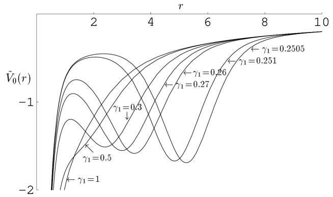
Figure 1: The potentials $\tilde{V}_{0}(r)$ for various values of $\gamma_{1}$.

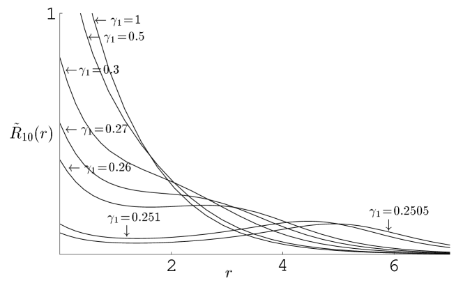
Figure 2: The ground states $\tilde{R}_{10}(r)$ for various values of $\gamma_{1}$.

The critical value of $\gamma_{1}\rightarrow 1/4$ is of interest. Our potential (3.1) then tends to:

$$\tilde{V}_{0}(r)=-\frac{2}{r}+\frac{16r(r+1)}{(2r^{2}+2r+1)^{2}}.$$ (3.2)

All the eigenvectors for $\gamma_{1}\rightarrow 1/4$ converge to some square-integrable function, except the first one (2.26) (missing vector) which then becomes non-normalizable. Therefore, the potential (3.2) is missing the lowest energy level comparing to the hydrogen atom. As immediately seen, this case reproduces the one previously found by Abraham and Moses by applying the Gelfand-Levitan method (see [6]). For $\gamma\neq 1/4$, the radial potentials (3.1), as far as we know, have not been known before.

Acknowledgements.

I am very much indebted to Dr. Bogdan Mielnik for lending me the manuscript of his work. Thanks are also due to all my Colleagues at the Departamento de Física del CINVESTAV for their interest in this work and stimulating discussions.

References

- [1] L. Infeld and T.E. Hull, Rev. Mod. Phys. 23, 21 (1951).
- [2] J. Plebañski, Notes from lectures on elementary quantum mechanics, CINVESTAV, México (1966).
- [3] M. Moshinsky, The harmonic oscillator in modern physics, in From atoms to quarks, Gordon and Breach, New York (1969).
- [4] D. Basu and K.B. Wolf, J. Math. Phys. 24, 478 (1983).
- [5] B. Mielnik, J. Math. Phys. 25, 3387 (1984).
- [6] P.B. Abraham and H.E. Moses, Phys. Rev. A 22, 1333 (1980).
- [7] M.M. Nieto and V.P. Gutschick, Phys. Rev. D 23, 922 (1981).
- [8] M.M. Nieto, Phys. Rev. D 24, 1030 (1981).