The interference of a nonclassical light pulse with a coherent one
and the sub-Poissonian statistics formation.

Abstract

Using the theoretical model of the optical beam-splitter, the interference of the self-phase modulated ultrashort light pulse (SPM-USP) with the coherent one is investigated. It is found that, the choice of the coefficient of transmission of the beam-splitter allows one to get the spectra of quadrature fluctuations with forms of interest to us. It is shown that, the choice of the geometrical phase gives one the control of the position of the ellipse of squeezing in the quadrature space $XY$. The extended Mandel parameter is introduced and the photon statistics is scanned at all frequencies. It is established that, the sub- and super-Poissonian statistics formation can be determined by the choice of the nonlinear phase addition and initial linear phase shift between pulses. It is also shown that, the self-phase modulation (SPM) leads to the additional modulation of total photon number at the outputs of the beam-splitter.

]

I Introduction

The formation of ultrashort light pulses (USPs) with suppressed photon fluctuations remains in the focus of considerable attention. The formation and application of USPs in a nonclassical state make possible to combine in experiments a high time resolution with a low level of fluctuations. There are some methods to obtain the USPs in the nonclassical state.

Parametric amplification is a technique that is most extensively used for the production of the USPs in the nonclassical state. In the case of degenerate three-frequency parametric amplification, quadrature-squeezed light is produced. However, this light is found to have super-Poissonian photon statistics directly at the output of an amplifier, and needs interferometers to transform it to one with sub-Poissonian statistics.

One of the most interesting methods for production of USPs in the nonclassical state is the self-phase modulation (SPM) in a nonlinear inertial medium [1, 2, 3]. In this case the USP in the quadrature-squeezing state can be formed with conservation of the photon statistics [4]. The SPM itself is not accompanied by a change in photon statistics. With the aid of nonlinear optical devices in the presence of the SPM one can obtain light with sub-Poissonian photon statistics (see [5]).

For the first time in [6] a simple method for the production of the USPs with suppressed photon number fluctuations was considered, which is based on the SPM of a USP in a nonlinear inertial medium and subsequent transmission of a pulse through a dispersive optical element. The accurate calculation of this process was conducted making use of technique developed in [1, 2, 3].

In the present paper, the interference of the SPM-USP with the coherent USP is analysed. The interference is realized using the optical beam-splitter and the process under consideration is analysed in the framework of the quantum theory of SPM of USPs developed in [1, 2, 3].

The aim of the present article is to analyse the spectra of quantum fluctuations of quadrature components and the spectra of quantum fluctuations of the photon number of the pulses at the outputs of an optical beam-splitter. An extended Mandel parameter will be introduced in order to analyse the photon statistics at all frequencies. The modulation of the total photon number will be analysed too.

II Spectra of quantum fluctuations of quadratures of SPM-USPs

For the first time in [1, 2, 3] the consequently quantum theory of self-action of USPs in nonlinear inertial medium based on the algebra of time-dependent Bose-operators has been developed. When analysed from the quantum point of view, SPM of USPs is described by the expression [1, 2, 3]

$$\hat{A}(t,z)=e^{\hat{O}(t)}\,\hat{A}_{0}(t),$$ (1)

where $\hat{A}(t,z)$ is the annihilation Bose-operator in the given cross section $z$ of the nonlinear inertial medium, $\hat{O}(t)=i\gamma q[\hat{n}_{0}(t)]$ and $\gamma q[\hat{n}_{0}(t)]$ is nonlinear phase incursion. The permutation relation takes place:

$$\hat{A}_{0}(t_{1})e^{\hat{O}(t_{2})}=e^{\hat{O}(t_{2})+{G}(t_{2}-t_{1})}\hat{A}_{0}(t_{1}),$$ (2)

and the theorem of the normal ordering is valid

$$e^{\hat{O}(t)}=\hat{\mathbf{N}}\exp\left\{\int_{-\infty}^{\infty}\left[e^{{\mathcal{H}}(\theta)}-1\right]\hat{n}_{0}(t-\theta\tau_{r})d\theta\right\},$$ (3)

where ${G}(t_{2}-t_{1})=i\gamma h(t_{2}-t_{1})$, $h(t)=H(|t|)$, ${\mathcal{H}}(\theta)=i\gamma\widetilde{h}(\theta)$, $\widetilde{h}(\theta)=\tau_{r}h(\theta\tau_{r})$, $\tau_{r}$ is the relaxation time of the nonlinear medium and $\hat{\mathbf{N}}$ is the operator of normal ordering. Here $H(t)$ represents the nonlinear response function of the nonlinear medium ($H(t)>0$ for $t>0$ and $H(t)=0$ for $t<0$). Eqs.(1-3) are written in the moving frame $t=t^{\prime}-z/u$, $z=z^{\prime}$, where $t^{\prime}$ is the time measured in co-moving frame and $u$ is the speed of a pulse in the nonlinear inertial medium.

The quadrature components of the light pulse are defined by the expressions

$$\hat{X}(t,z) = [\hat{A}(t,z)+\hat{A}^{+}(t,z)]/2,$$ (5)

$$\hat{Y}(t,z) = [\hat{A}(t,z)-\hat{A}^{+}(t,z)]/2i,$$ (6)

and for average values of quadratures we have [1, 2, 3]

$$\langle\hat{X}(t,z)\rangle = |\alpha_{0}(t)|e^{-\mu(t)}\cos{\Phi(t)},$$ (8)

$$\langle\hat{Y}(t,z)\rangle = |\alpha_{0}(t)|e^{-\mu(t)}\sin{\Phi(t)}.$$ (9)

In (8-9) we denoted $\Phi(t)=\psi(t)+\varphi(t)$, $\psi(t)=2\gamma|\alpha_{0}(t)|^{2}=2\gamma\bar{n}_{0}(t)$ and $\mu(t)=\gamma^{2}\bar{n}_{0}(t)=\gamma\psi(t)/2$. The correlation functions of the quadrature components must be introduced as [1, 2, 3]

$$R_{X}(t,t\smash{+}\tau)\!=\!\frac{1}{2}\!\! \Bigl{[} \!\!\!\langle\hat{X}(t,z)\hat{X}(t\smash{+}\tau,z)\rangle\smash{+}\langle\hat{X}(t\smash{+}\tau,z)\hat{X}(t,z)\rangle$$ (11)

$$- 2\langle\hat{X}(t,z)\rangle\langle\hat{X}(t\smash{+}\tau,z)\rangle\Bigl{]},$$ (12)

$$R_{Y}(t,t\smash{+}\tau)\!=\!\frac{1}{2}\!\! \Bigl{[} \!\!\!\langle\hat{Y}(t,z)\hat{Y}(t\smash{+}\tau,z)\rangle\smash{+}\langle\hat{Y}(t\smash{+}\tau,z)\hat{Y}(t,z)\rangle$$ (13)

$$- 2\langle\hat{Y}(t,z)\rangle\langle\hat{Y}(t\smash{+}\tau,z)\rangle\Bigl{]},$$ (14)

where $\tau=t_{1}\smash{-}t$ ($t_{1}$ is an arbitrary moment of time, $t_{1}>t$). Using algebra of time-dependent Bose-operators (see (2-3)) for the correlation functions we find

$$R_{X}(t,t+\tau)=\frac{1}{4}\Bigl{\{}\delta(\tau) - \psi(t)h(\tau)\sin{2\Phi(t)}$$ (16)

$$+ \psi^{2}(t)g(\tau)\sin^{2}{\Phi(t)}\Bigl{\}},$$ (17)

$$R_{Y}(t,t+\tau)=\frac{1}{4}\Bigl{\{}\delta(\tau) + \psi(t)h(\tau)\sin{2\Phi(t)}$$ (18)

$$+ \psi^{2}(t)g(\tau)\cos^{2}{\Phi(t)}\Bigl{\}},$$ (19)

where we denoted $h(\tau)\smash{=}\tau^{-1}_{r}\exp{\{-|\tau|/\tau_{r}\}}$, $g(\tau)=\tau^{-1}_{r}(1+|\tau|/\tau_{r})\exp{\{-|\tau|/\tau_{r}\}}$ and considered that nonlinear inertial medium is of a Kerr type. To get the expressions (17-19), the approximations $\tau_{r}\ll\tau_{p}$ , $\gamma\ll 1$ have been used ($\tau_{p}$ is the pulse duration). The spectra of the fluctuations of quadrature components are

$$S_{X}(\Omega,t)=\frac{1}{4}\bigl{[}1 - 2\psi(t)L(\Omega)\sin{2\Phi(t)}$$ (22)

$$+4\psi^{2}(t)L^{2}(\Omega)\sin^{2}{\Phi(t)}\bigl{]},$$

$$S_{Y}(\Omega,t)=\frac{1}{4}\bigl{[}1 + 2\psi(t)L(\Omega)\sin{2\Phi(t)}$$ (24)

$$+4\psi^{2}(t)L^{2}(\Omega)\cos^{2}{\Phi(t)}\bigl{]},$$

where we denoted $\Omega=\omega\tau_{r}$ and $L(\Omega)=1/[1+\Omega^{2}]$. At initial phase chosen optimal at the frequency $\Omega_{0}$ (see [1, 2, 3])

$$\varphi_{0}(t)=\frac{1}{2}\arctan{\left\{\frac{1}{\psi(t)L(\Omega_{0})}\right\}}-\psi(t)$$ (25)

the spectra (22-24) have the forms

$$S_{X}(\Omega_{0},t) = \frac{1}{4}\bigl{[}\sqrt{1+\psi^{2}(t)L^{2}(\Omega_{0})}-\psi(t)L(\Omega_{0})\bigl{]}^{2},$$ (27)

$$S_{Y}(\Omega_{0},t) = \frac{1}{4}\bigl{[}\sqrt{1+\psi^{2}(t)L^{2}(\Omega_{0})}+\psi(t)L(\Omega_{0})\bigl{]}^{2}.$$ (28)

At any frequency $\Omega$ the spectra (22-24) are given by:

$$S_{X}(\Omega,t) = S_{X}(\Omega_{0},t)+\frac{1}{2}\psi(t)[L(\Omega)-L(\Omega_{0})]$$ (32)

$$\times\Bigl{\{}[L(\Omega)\smash{+}L(\Omega_{0})]\psi(t)\smash{-}[1\smash{+}(L(\Omega)\smash{+}L(\Omega_{0}))$$

$$~{}\times L(\Omega_{0})\psi^{2}(t)][1\smash{+}\psi^{2}(t)L^{2}(\Omega)]^{-1/2}\Bigl{\}},$$

$$S_{Y}(\Omega,t) = S_{Y}(\Omega_{0},t)+\frac{1}{2}\psi(t)[L(\Omega)-L(\Omega_{0})]$$ (35)

$$\times\Bigl{\{}[L(\Omega)\smash{+}L(\Omega_{0})]\psi(t)\smash{+}[1\smash{+}(L(\Omega)\smash{+}L(\Omega_{0}))$$

$$~{}\times L(\Omega_{0})\psi^{2}(t)][1\smash{+}\psi^{2}(t)L^{2}(\Omega)]^{-1/2}\Bigl{\}}.$$

The spectra of the quantum fluctuations of squeezed $X$-quadrature at the initial phase chosen optimal at the reduced frequency $\Omega_{0}=0$ are displayed in Fig.1.

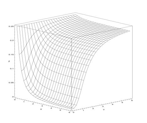
FIG. 1.: Dispersion [Z] of the $X$-quadrature component of a pulse at time $t\smash{=}0$ as a function of the maximum nonlinear phase $\psi(0)$ [X] and the reduced frequency $\Omega\smash{=}\omega\tau_{r}$ [Y], at values of the phase of the pulse which are optimal for $\Omega_{0}\smash{=}0$.

From Fig.1 one can see that the squeezing of quantum fluctuations is greatest at the frequency for which the phase of the initial pulse was chosen optimal. In addition, in [1, 2, 3] have been shown that the spectra of quantum fluctuations of quadrature components can be controlled by the choice of the phase of the initial light pulse and that, at the initial phase chosen optimal at the frequency $\Omega_{0}=1$, the squeezing of quadrature component $X$ is maximum at frequencies $\omega\approx 1/\tau_{r}$ for $\psi(t)>1$.

The choice of the optimal phase as (25) means that in the quadrature’s space $XY$ the big axis of the eclipse of squeezing is parallel with the $Y$ axis and consequently, the squeezing of the $X$ quadrature is maximum (see (32)). The transformation of the uncertainty region of quadrature fluctuations, from the circle for the initial coherent light pulse to the ellipse for the SPM-USP, always take place. The choice of the phase as (25) means the orientation of the system of quadrature squeezing observation $XY$ as the quantum fluctuations of $X$ quadrature are maximum suppressed.

III The interference of SPM-USP with a coherent one

In what follows we are interested in analysing of the interference between the SPM-USP and coherent one. As a theoretical model we use the model of the symmetric beam-splitter [7] (double reflection angle of the incident SPM-USP is $\pi/2$). The interference scheme is presented in Fig.2. The input-output operator transformations [7] at the output # $1$ are given by

$$\hat{B}_{1}(t) = i\sqrt{R}\,\hat{A}_{1}(t,l)+\sqrt{T}\,\hat{A}_{2}(t),$$ (37)

$$\hat{B}^{+}_{1}(t) = -i\sqrt{R}\,\hat{A}^{+}_{1}(t,l)+\sqrt{T}\,\hat{A}_{2}(t),$$ (38)

and at the output # 2 they are

$$\hat{B}_{2}(t) = \sqrt{T}\,\hat{A}_{1}(t,l)+i\sqrt{R}\,\hat{A}_{2}(t),$$ (40)

$$\hat{B}^{+}_{2}(t) = \sqrt{T}\,\hat{A}^{+}_{1}(t,l)-i\sqrt{R}\,\hat{A}^{+}_{2}(t),$$ (41)

where $l$ is the length of the nonlinear inertial medium and $R$ is the coefficient of reflection, $R+T=1$.

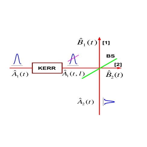
FIG. 2.: The scheme of the optical beam-splitter (BS) in which the interference between the nonclassical SPM-USP and coherent SPM is realized. [1] and [2] represent the BS outputs.

A The spectra of quantum fluctuations of quadratures at the beam-splitter output # $1$

We define the quadrature components at the output # $1$ of the beam splitter as (see (5-6))

$$\hat{\mathcal{X}}_{1}(t) = [\hat{B}_{1}(t)+\hat{B}^{+}_{1}(t)]/2,$$ (43)

$$\hat{\mathcal{Y}}_{1}(t) = [\hat{B}_{1}(t)-\hat{B}^{+}_{1}(t)]/2i.$$ (44)

For average values of the quadrature components (43-44) we find

$$\langle\hat{\mathcal{X}}_{1}(t)\rangle \smash{=} |\alpha_{0}(t)|e^{-\mu(t)}[\sqrt{T}\cos\varphi_{2}(t)\smash{-}\sqrt{R}\sin\Phi_{1}(t)],$$ (46)

$$\langle\hat{\mathcal{Y}}_{1}(t)\rangle \smash{=} |\alpha_{0}(t)|e^{-\mu(t)}[\sqrt{T}\sin\varphi_{2}(t)\smash{+}\sqrt{R}\cos\Phi_{1}(t)],$$ (47)

where $\Phi_{1}(t)=\psi(t)+\varphi_{1}(t)$, $\psi(t)=2\gamma\bar{n}_{1}(t)$, $\mu(t)=\gamma\psi(t)/2$ and $\varphi_{1}(t)$ is the initial phase of the pulse in nonlinear section. For the correlation functions of the quadrature components we have

$$R_{{\mathcal{X}}_{1}}(t,t+\tau)=\frac{1}{4}\Bigl{\{}\delta(\tau) + R\psi(t)h(\tau)\sin 2\Phi_{1}(t)$$ (49)

$$+ R\psi^{2}(t)g(\tau)\cos^{2}\Phi_{1}(t)\Bigl{\}},$$ (50)

$$R_{{\mathcal{Y}}_{1}}(t,t+\tau)=\frac{1}{4}\Bigl{\{}\delta(\tau) - R\psi(t)h(\tau)\sin 2\Phi_{1}(t)$$ (51)

$$+ R\psi^{2}(t)g(\tau)\cos^{2}\Phi_{1}(t)\Bigl{\}}.$$ (52)

For the spectra of quadrature fluctuations we find

$$S_{{\mathcal{X}}_{1}}(\Omega,t)=\frac{1}{4}\bigl{[}1 + 2R\psi(t)L(\Omega)\sin 2\Phi_{1}(t)$$ (55)

$$+4R\psi^{2}(t)L^{2}(\Omega)\cos^{2}\Phi_{1}(t)\bigl{]},$$

$$S_{{\mathcal{Y}}_{1}}(\Omega,t)=\frac{1}{4}\bigl{[}1 - 2R\psi(t)L(\Omega)\sin 2\Phi_{1}(t)$$ (57)

$$+4R\psi^{2}(t)L^{2}(\Omega)\sin^{2}\Phi_{1}(t)\bigl{]}.$$

At optimal phase (25) the spectra (55-57) take the forms

$$S_{{\mathcal{X}}_{1}}(\Omega_{0},t) = \frac{1}{4}\Bigl{\{}\bigl{[}\sqrt{1+\psi^{2}(t)L^{2}(\Omega_{0})}+R\psi(t)L(\Omega_{0})\bigl{]}^{2}$$ (60)

$$-\left(2R-1\right)^{2}\psi^{2}(t)L^{2}(\Omega_{0})\Bigl{\}},$$

$$S_{{\mathcal{Y}}_{1}}(\Omega_{0},t) = \frac{1}{4}\Bigl{\{}\bigl{[}\sqrt{1+\psi^{2}(t)L^{2}(\Omega_{0})}-R\psi(t)L(\Omega_{0})\bigl{]}^{2}$$ (62)

$$-\left(2R-1\right)^{2}\psi^{2}(t)L^{2}(\Omega_{0})\Bigl{\}}.$$

At any frequency $\Omega$ we have

$$S_{{\mathcal{X}}_{1}}(\Omega,t)\! = \!S_{{\mathcal{X}}_{1}}(\Omega_{0},t)+\frac{1}{2}\,R\,\psi(t)[L(\Omega)-L(\Omega_{0})]$$ (66)

$$\times\Bigl{\{}[L(\Omega)+L(\Omega_{0})]\psi(t)+[1+(L(\Omega)\smash{+}L(\Omega_{0}))$$

$$~{}\times L(\Omega_{0})\psi^{2}(t)][1\smash{+}\psi^{2}(t)L^{2}(\Omega_{0})]^{-1}\Bigl{\}},$$

$$S_{{\mathcal{Y}}_{1}}(\Omega,t)\! = \!S_{{\mathcal{Y}}_{1}}(\Omega_{0},t)+\frac{1}{2}\,R\,\psi(t)[L(\Omega)-L(\Omega_{0})]$$ (69)

$$\times\Bigl{\{}[L(\Omega)+L(\Omega_{0})]\psi(t)-[1+(L(\Omega)\smash{+}L(\Omega_{0}))$$

$$~{}\times L(\Omega_{0})\psi^{2}(t)][1\smash{+}\psi^{2}(t)L^{2}(\Omega_{0})]^{-1}\Bigl{\}}.$$

As one can see from (66-69) the interference of the SPM-USP with the coherent USP does not influence the quadrature squeezing of the SPM-USP. The choice of the coefficient of reflection $R$ of the beam-splitter allows us to receive the spectra of squeezing (see (66-69)) of interest to us. One can conclude that, the lost of photons from SPM-USP as a result of division in the beam-splitter is follows by the reduction of squeezing. In fact this lost is compensated by the coherent USP. The spectra of quantum fluctuations of ${\mathcal{Y}}_{1}$ quadrature at time $t=0$ as a function of maximum nonlinear phase $\psi(0)=\psi_{0}$ and the reduced frequency $\Omega$ in the case of the $50\%$ beam-splitter ($R=T=1/2$) is displayed in Fig.3. On Fig.3 one can see that, in this case the squeezing is reduced at one half.

Also, it is important to remark that, as a result of symmetric reflection the squeezing from the $X$ quadrature is moved in the $Y$ quadrature. This means that the ellipse of squeezing is moved in the $XY$ frame with an angle equal to double reflection angle. From theoretical point of view this is expressed by the presence of the index $i=\exp{(i\pi/2)}$ in the (37-38) and (40-41). The double angle of reflection can be interpreted as a geometrical phase. The choice of the position of the beam-splitter relative to direction of propagation of the SPM-USP allows us to control the position of the ellipse of squeezing in the $XY$ frame.

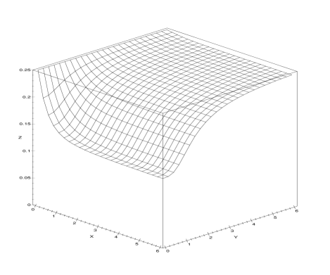
FIG. 3.: Dispersion [Z] of the ${\mathcal{Y}}_{1}$- quadrature component of a pulse at time $t\smash{=}0$ as a function of the maximum nonlinear phase $\psi(0)$ [X] and the reduced frequency $\Omega\smash{=}\omega\tau_{r}$ [Y], at values of the phase of the pulse which are optimal for $\Omega_{0}\smash{=}0$ ($R=T=1/2$).

B The spectra of quantum fluctuations of quadratures at the beam-splitter output # $2$

At the output # $2$ the quadrature components are defined as

$$\hat{\mathcal{X}}_{2}(t) = [\hat{B}_{2}(t)+\hat{B}^{+}_{2}(t)]/2,$$ (71)

$$\hat{\mathcal{Y}}_{2}(t) = [\hat{B}_{2}(t)-\hat{B}^{+}_{2}(t)]/2i.$$ (72)

For the average values of quadrature components we find

$$\langle\hat{\mathcal{X}}_{2}(t)\rangle \smash{=} |\alpha_{0}(t)|e^{-\mu(t)}[\sqrt{T}\cos\Phi_{1}(t)\smash{-}\sqrt{R}\sin\varphi_{2}(t)],$$ (74)

$$\langle\hat{\mathcal{Y}}_{2}(t)\rangle \smash{=} |\alpha_{0}(t)|e^{-\mu(t)}[\sqrt{T}\sin\Phi_{1}(t)\smash{+}\sqrt{R}\cos\varphi_{2}(t)].$$ (75)

Leaving out the preliminary accounts for the correlation functions of the quadrature components we get

$$R_{{\mathcal{X}}_{2}}(t,t+\tau)=\frac{1}{4}\Bigl{\{}\delta(\tau) - T\psi(t)h(\tau)\sin 2\Phi_{1}(t)$$ (77)

$$+ T\psi^{2}(t)g(\tau)\cos^{2}\Phi_{1}(t)\Bigl{\}},$$ (78)

$$R_{{\mathcal{Y}}_{2}}(t,t+\tau)=\frac{1}{4}\Bigl{\{}\delta(\tau) + T\psi(t)h(\tau)\sin 2\Phi_{1}(t)$$ (79)

$$+ T\psi^{2}(t)g(\tau)\cos^{2}\Phi_{1}(t)\Bigl{\}}.$$ (80)

In consequence, for the spectra of quantum fluctuations of quadratures we have

$$S_{{\mathcal{X}}_{2}}(\Omega,t)=\frac{1}{4}\bigl{[}1 - 2T\psi(t)L(\Omega)\sin 2\Phi_{1}(t)$$ (83)

$$+4T\psi^{2}(t)L^{2}(\Omega)\sin^{2}\Phi_{1}(t)\bigl{]},$$

$$S_{{\mathcal{Y}}_{2}}(\Omega,t)=\frac{1}{4}\bigl{[}1 + 2T\psi(t)L(\Omega)\sin 2\Phi_{1}(t)$$ (85)

$$+4T\psi^{2}(t)L^{2}(\Omega)\cos^{2}\Phi_{1}(t)\bigl{]}.$$

The spectra (83-85) at optimal phase (25) are:

$$S_{{\mathcal{X}}_{2}}(\Omega_{0},t) = \frac{1}{4}\Bigl{\{}\bigl{[}\sqrt{1+\psi^{2}(t)L^{2}(\Omega_{0})}-T\psi(t)L(\Omega_{0})\bigl{]}^{2}$$ (88)

$$-(2T-1)^{2}\psi^{2}(t)L^{2}(\Omega_{0})\Bigl{\}},$$

$$S_{{\mathcal{Y}}_{2}}(\Omega_{0},t) = \frac{1}{4}\Bigl{\{}\bigl{[}\sqrt{1+\psi^{2}(t)L^{2}(\Omega_{0})}+T\psi(t)L(\Omega_{0})\bigl{]}^{2}$$ (90)

$$-(2T-1)^{2}\psi^{2}(t)L^{2}(\Omega_{0})\Bigl{\}}.$$

At any frequency $\Omega$ the spectra (83-85) take the forms

$$S_{{\mathcal{X}}_{2}}(\Omega,t)\! = \!S_{{\mathcal{X}}_{2}}(\Omega_{0},t)+\frac{1}{2}\,T\,\psi(t)[L(\Omega)-L(\Omega_{0})]$$ (94)

$$\times\Bigl{\{}[L(\Omega)+L(\Omega_{0})]\psi(t)-[1+(L(\Omega)\smash{+}L(\Omega_{0}))$$

$$~{}\times L(\Omega_{0})\psi^{2}(t)][1\smash{+}\psi^{2}(t)L^{2}(\Omega_{0})]^{-1}\Bigl{\}},$$

$$S_{{\mathcal{Y}}_{2}}(\Omega,t)\! = \!S_{{\mathcal{Y}}_{2}}(\Omega_{0},t)+\frac{1}{2}\,T\,\psi(t)[L(\Omega)-L(\Omega_{0})]$$ (97)

$$\times\Bigl{\{}[L(\Omega)+L(\Omega_{0})]\psi(t)+[1+(L(\Omega)\smash{+}L(\Omega_{0}))$$

$$~{}\times L(\Omega_{0})\psi^{2}(t)][1\smash{+}\psi^{2}(t)L^{2}(\Omega_{0})]^{-1}\Bigl{\}}.$$

As already have been remarked in the previous analyse, the spectra of quadrature fluctuations can be controlled by the choice of the coefficients of the beam-splitter (see (66-69)). It is interesting to remark that, in case of the symmetric $50\%$ beam-splitter, the squeezing of quadrature fluctuations at output # $2$ is present only in the ${\mathcal{X}}_{2}$ quadrature and it is reduced at one half (see (94-97)). Since the geometrical phase is equal to $0$ in the analysed case (the refracted part of the SPM-USP does not change the direction of propagation in comparison with the initial SPM-USP) the ellipse of squeezing does not change this initial position in the $XY$ frame and has the big axis parallel to $Y$ axis.

IV The spectra of fluctuations of photon number and the statistics

We introduce the correlation function of photon number at the output number $j$ ($j=\overline{1,2}$) in the following symmetric form

$$R_{N,j}(t_{1},t_{2}) = \frac{1}{2}\Bigl{[}\langle\hat{N}_{j}(t_{1})\hat{N}_{j}(t_{2})\rangle+\langle\hat{N}_{j}(t_{2})\hat{N}_{j}(t_{1})\rangle$$ (99)

$$-2\langle\hat{N}_{j}(t_{1})\rangle\langle\hat{N}_{j}(t_{2})\rangle\Bigl{]}.$$

To simplify the accounts we consider that the initial pulses have the identical average values of the photon number ($\bar{n}_{1}(t)=\bar{n}_{2}(t)=\bar{n}_{0}(t)$). Using the algebra of time-dependent Bose-operators (2-3) for the correlation functions we get

$$R_{N,1}(t,t+\tau)\! = \!\bar{n}_{0}(t)\Bigl{[}\delta(\tau)-2R\sqrt{RT}\psi(t)h(\tau)\cos{\widetilde{\Phi}(t)}$$ (103)

$$+RT\psi(t)h(\tau)\sin{2\widetilde{\Phi}(t)}$$

$$~{}+RT\psi^{2}(t)g(\tau)\cos^{2}{\widetilde{\Phi}(t)}\Bigl{]},$$

$$R_{N,2}(t,t+\tau)\! = \!\bar{n}_{0}(t)\Bigl{[}\delta(\tau)+2T\sqrt{RT}\psi(t)h(\tau)\cos{\widetilde{\Phi}(t)}$$ (106)

$$+RT\psi(t)h(\tau)\sin{2\widetilde{\Phi}(t)}$$

$$~{}+RT\psi^{2}(t)g(\tau)\cos^{2}{\widetilde{\Phi}(t)}\Bigl{]}.$$

where in (103-106) is denoted $\tau=t_{1}\smash{-}t$ (see (12-14)), $\widetilde{\Phi}(t)=\psi(t)+\Delta\varphi(t)$, $\Delta\varphi(t)=\varphi_{1}(t)-\varphi_{2}(t)$. In the case of the symmetrical $50\%$ beam-splitter, the spectra of quantum fluctuations of the photon number at the measured time ${\mathcal{T}}$ have the forms

$$S_{{\mathcal{T}},1}(\Omega,t)\! = \!\bar{{\mathcal{N}}}+\bar{n}_{0}(t)\psi(t)L(\Omega)\left(\frac{\mathcal{T}}{\tau_{p}}\right)\biggl{[}-\cos{\widetilde{\Phi}(t)}$$ (109)

$$+\frac{1}{2}\sin{2\widetilde{\Phi}(t)}+\psi(t)L(\Omega)\cos^{2}{\widetilde{\Phi}(t)}\biggl{]},$$

$$S_{{\mathcal{T}},2}(\Omega,t)\! = \!\bar{{\mathcal{N}}}+\bar{n}_{0}(t)\psi(t)L(\Omega)\left(\frac{\mathcal{T}}{\tau_{p}}\right)\biggl{[}\cos{\widetilde{\Phi}(t)}$$ (111)

$$+\frac{1}{2}\sin{2\widetilde{\Phi}(t)}+\psi(t)L(\Omega)\cos^{2}{\widetilde{\Phi}(t)}\biggl{]},$$

where $\bar{{\mathcal{N}}}=\int_{-\infty}^{\infty}\bar{n}_{0}(t)dt$ is the total photon number of the initial coherent USP. An extended Mandel parameter at all frequencies describing the photon statistics at measurement time ${\mathcal{T}}$ can be introduced as

$$Q_{{\mathcal{T}},1}(\Omega,t) = \varepsilon_{{\mathcal{T}},1}(\Omega,t)\bigl{/}\bar{n}_{0}(t)$$ (113)

$$= \psi(t)L(\Omega)\left(\frac{\mathcal{T}}{\tau_{p}}\right)\biggl{[}-\cos{\widetilde{\Phi}(t)}\smash{+}\frac{1}{2}\sin{2\widetilde{\Phi}(t)}$$ (115)

$$~{}+\psi(t)L(\Omega)\cos^{2}{\widetilde{\Phi}(t)}\biggl{]},$$

$$Q_{{\mathcal{T}},2}(\Omega,t) = \varepsilon_{{\mathcal{T}},2}(\Omega,t)\bigl{/}\bar{n}_{0}(t)$$ (116)

$$= \psi(t)L(\Omega)\left(\frac{\mathcal{T}}{\tau_{p}}\right)\biggl{[}\cos{\widetilde{\Phi}(t)}\smash{+}\frac{1}{2}\sin{2\widetilde{\Phi}(t)}$$ (118)

$$~{}+\psi(t)L(\Omega)\cos^{2}{\widetilde{\Phi}(t)}\biggl{]},$$

where in (115-118) we denoted $\varepsilon_{{\mathcal{T}},j}(\Omega,t)\smash{=}S_{{\mathcal{T}},j}(\Omega,t)\smash{-}\bar{{\mathcal{N}}}$.

The statistics of photon number can be controlled by the choice of the nonlinear phase addition $\psi(t)$ and linear phase shift $\triangle\varphi(t)$. The dependence of the extended Mandel parameter $Q_{{\mathcal{T}},1}(\Omega,t)$ at time $t=0$, ${\mathcal{T}}/\tau_{p}=1/10$ and $\triangle\varphi(t)\smash{=}\pi/2$ on $\psi_{0}$ and $\Omega$ is displayed in Fig.4.

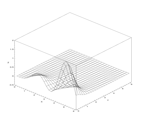
FIG. 4.: The dependence of the extended Mandel parameter $Q_{{\mathcal{T}},1}(\Omega,0)$ [Z] on the maximum nonlinear phase $\psi_{0}$ [X] and the reduced frequency $\Omega\smash{=}\omega\tau_{r}$ [Y] at ${\mathcal{T}}/\tau_{p}=1/10$ and $\triangle\varphi(t)=\pi/2$.

As follows from Fig.4, for different values of the nonlinear phase addition, the statistics of photon number can be as super-Poissonian as sub-Poissonian. The maximum increase or decrease of photon number fluctuations take place around the central frequency $\Omega\smash{=}0$. From Fig.4 it follows that in case $\triangle\varphi(t)=\pi/2$ the first suppression of the photon number fluctuations takes place around $\psi(t)=3.5$ and it can be observed at all frequencies from $0$ to $\omega\approx 2/\tau_{r}$.

It is important to mention that, if the radiation is monochromatic, the formulas (115-118) remain valid. In this case, there are no second and third terms in (115-118) and the reduced frequency $\Omega\smash{=}0$, as since all the photons have the same frequency. The presence of these terms is connected with the correlation between modes of SPM-USP (see [2]) and in consequence, the quantum fluctuations of the photon number for the pulse field will be “smoothed-out” at the frequency $\Omega\smash{=}0$ in comparison with the monochromatic radiation.

V The modulation of the total photon number

Let us introduce the photon number operator at the measurement time ${\mathcal{T}}$ [6]

$$\hat{{\mathcal{N}}}_{{\mathcal{T}},j}(t)=\int_{t-{\mathcal{T}}/2}^{t+{\mathcal{T}}/2}\hat{N}_{j}(t^{{}^{\prime}})dt^{{}^{\prime}},$$ (119)

where

$$\hat{N}_{j}(t)=\hat{B}^{+}_{j}(t)\hat{B}_{j}(t).$$ (120)

To simplify the accounts, in following we consider that $\bar{n}_{1}(t)=\bar{n}_{2}(t)=\bar{n}_{0}(t)$ and then we get

$$\langle\hat{\mathcal{N}}_{{\mathcal{T}},1}(t)\rangle\! = \!{\mathcal{T}}\bar{n}_{0}(t)\left\{1\smash{-}2\sqrt{RT}\,\sin{\left[\psi(t)\smash{+}\triangle\varphi(t)\right]}\right\},$$ (122)

$$\langle\hat{\mathcal{N}}_{{\mathcal{T}},2}(t)\rangle\! = \!{\mathcal{T}}\bar{n}_{0}(t)\left\{1\smash{+}2\sqrt{RT}\,\sin{\left[\psi(t)\smash{+}\triangle\varphi(t)\right]}\right\}.$$ (123)

where $\bar{n}_{0}(t)=\bar{n}_{0}\rho(t)$ and $\rho(t)$ is the envelope of the pulse. As can be seen from (122-123), for different values of the linear phase shift $\triangle\varphi(t)$ of the initial coherent light pulses, all photons can be distributed only in one of the outputs of the beam-splitter. This property is specific for the quantum interference only and has no classical analogue.

Let us introduce the total number operator at the beam-splitter output # $1$ as

$$\hat{{\mathcal{N}}}_{1}=\int_{-\infty}^{\infty}\hat{N}_{1}(t)dt,$$ (124)

and for its average value we obtain

$$\bar{{\mathcal{N}}}_{1}=\bar{{\mathcal{N}}}\left[1-2\sqrt{RT}\,\frac{\sin(\psi_{0}/4)}{\psi_{0}/4}\,\sin{\left(\frac{\psi_{0}}{4}+\triangle\varphi\right)}\right].$$ (125)

To get (125) we considered that the initial pulses are quite Gaussian, their envelopes having the form $\rho(t)\approx\exp{\left\{-t^{2}\bigl{/}2\tau^{2}_{p}\right\}}/\sqrt{2}$, and that $\triangle\varphi(t)\smash{=}\triangle\varphi$ is a constant.

The dependence of $\bar{\mathcal{N}}_{1}/\bar{{\mathcal{N}}}$ at maximum nonlinear phase addition $\psi_{0}$ for 50% beam-splitter and $\triangle\varphi\smash{=}0$ is displayed in Fig.5.

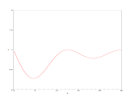
FIG. 5.: The dependence of $\bar{\mathcal{N}}_{1}/\bar{{\mathcal{N}}}$ [Y] on the maximum nonlinear phase $\psi_{0}$ [X] for $\triangle\varphi=0$.

As follows from (125) the SPM process leads to the additional modulation of the total photon number. In consequence, the choice of the maximum nonlinear phase addition $\psi_{0}$ and the initial phase shift $\triangle\varphi$ allows us to control the total photon number at the outputs of the beam-splitter.

VI Discussions and conclusions

The analyse of the interference process of the SPM-USP with coherent USP, based on the algebra of time-dependent Bose-operators, allows us to understand in which way the interference leads to the sub- and super-Poissonian photon statistics formation. Analysing the spectra of quantum fluctuations of quadrature components was concluded that, the position of the optical beam-splitter plays an important role in the quadrature squeezing observation. The initial phase, chosen optimal for a determined frequency plays a role of the phase of reference. Its choice means that, the $XY$ frame is placed so as the observed squeezing of quadrature $X$ is maximum. As a result of reflection of the SPM-USP at the beam-splitter, the ellipse of squeezing will move itself in the $XY$ frame with an angle equal to the geometrical phase. The geometrical phase can take the values for which the squeezing cannot be observed in $X$ or $Y$ quadratures. Let us take into consideration the case in which we get the initial phase of the light pulse in the nonlinear section arbitrary. In this case the ellipse of squeezing is located arbitrary in the $XY$ frame and it is possible do not observe the squeezing of quadrature fluctuations in the measurements. In case we chose the initial phase optimal, we locate the ellipse of squeezing in the $XY$ frame so as the small axis of the ellipse will lie along the $X$ axis. In consequence, the observed squeezing of $X$ quadrature fluctuations is maximum. If we do not know the position of the ellipse in the $XY$ frame (taking the initial phase arbitrary), then rotating the beam-splitter we can orientate the $XY$ frame so as the ellipse of squeezing can be displayed with small axis along $X$ axis and the squeezing of the $X$ quadrature fluctuations can be observed.

Up to now, it is considered that, after reflection from the beam-splitter, the squeezing of the quadrature fluctuations can be affected and complete disappeared as a result of the vacuum fluctuations participation at the other input of the beam-splitter. This interpretation is not quite correct. It is important to mention that, the presence of vacuum fluctuations was already taken into account when the SPM process in the nonlinear inertial medium was analysed from quantum point of view [2].

The presented in the recent work analyse gives the indication about the use of the nonclassical light pulses in gravitational wave detection. There are two points of interest. One is represented by the choice of the initial phase of a pulse at the input in nonlinear inertial medium which will determine the position of the ellipse of squeezing of quadrature fluctuations in the $XY$ frame. This optimal phase must be interpreted as the phase of reference. Other point is represented by the reflection of the SPM-USP from the surfaces, as since the addition of the geometrical phase will rotate the ellipse in the $XY$ frame consequently. These points must be taken into account when the experiments for gravitational wave detection are implemented using the USP in nonclassical state.

The extended Mandel parameter is introduced and the photon statistics is scanned at all frequencies. It is shown that, the statistics of the photon number can be controlled by choice of the nonlinear phase addition and the linear phase shift of the initial coherent light pulses. The choice of the linear phase shift represents an effective method of control of the sub- or super-Poissonian statistics formation and of the modulation of the total photon number.

It is interesting to mention that, the analyse of the interference process between two SPM-USPs can leads to the determination of the evolution of the linear parameters of the ellipse of squeezing as a functions of the nonlinear phase addition. This analyse will be the subject of another publication.

The author is grateful to S. Codoban (JINR, Dubna) for useful discussions and rendered help.

REFERENCES

• [1] A.S. Chirkin and F. Popescu, quant-ph/0003027.
• [2] F. Popescu and A.S. Chirkin, quant-ph/0003028.
• [3] F. Popescu and A.S. Chirkin, Pisma Zh. Eksp. Teor. Fiz, 69, 481, (1999), [JETP Lett. 69, 516 (1999)].
• [4] M. Kitagava and Y. Yamamoto, Phys. Rev. A, 34, 3974 (1986).
• [5] S.A. Akhmanov, A.V. Belinskii, A.S. Chirkin, in Novye Fizicheskie Printsipy Opticeskoi Obrabotki Informatsii (New Physics Methods of Optical Information Processing) (Eds S.A. Akhmanov, M.A. Vorontsov) (Moscow: Nauka, 1990), pp 83-194.
• [6] F. Popescu and A.S. Chirkin, Kvant. Elektron. (Moscow), 28, 61 (1999) [Sov. J. of Quant. Electron. 29, 61 (1999)], [ Enlarged version in quant-ph/0003042 ].
• [7] Z.Y. Ou, C.K. Hong and L. Mandel, Opt. Commun., 63, 118 (1987).