From the quantum Zeno to the inverse quantum Zeno effect

Abstract

The temporal evolution of an unstable quantum mechanical system undergoing repeated measurements is investigated. In general, by changing the time interval between successive measurements, the decay can be accelerated (inverse quantum Zeno effect) or slowed down (quantum Zeno effect), depending on the features of the interaction Hamiltonian. A geometric criterion is proposed for a transition to occur between these two regimes.

The temporal evolution of the survival probability of a quantum mechanical unstable system is characterized by a short-time quadratic behavior, an intermediate approximately exponential decay and a long-time power tail [1]. The short-time region has attracted the attention of physicists since quite some time ago, because it leads, under particular conditions, to the quantum Zeno effect (QZE) [2], by which frequent observations slow down the evolution. However, it has recently been pointed out that by exploiting the short-time features of the quantal evolution one can also accelerate the decay [3, 4, 5, 6]. We will call this phenomenon inverse quantum Zeno effect (IZE).

In this Letter we shall analyze how the Zeno–inverse Zeno transition takes place when the frequency of observations is changed. For an oscillating quantum mechanical system, whose Poincaré time is finite, it is not difficult to obtain a QZE. On the other hand, when the system is unstable, the situation is much more interesting and involved: in general, one can obtain both a QZE or an IZE depending on the features of the interaction Hamiltonian.

Let us summarize the main features of the QZE. Prepare, at $t=0$, a quantum system in some (normalizable) initial state. A QZE typically arises if one performs a series of “measurements,” at time intervals $\tau$, in order to ascertain whether the system is still in its initial state. If $P(t)$ denotes the undisturbed survival probability in the initial state, after the $N$th measurements the survival probability reads

$$P^{(N)}(t)=P(\tau)^{N}\equiv\exp[-\gamma(\tau)t],$$ (1)

where $t=N\tau$ is the total duration of the experiment and we have introduced an effective decay rate $\gamma(\tau)$, which is defined through the last equality. Notice that the far r.h.s. represents an exponential “interpolation” of $P^{(N)}(t)$ and that $\gamma$ is in general $\tau$ dependent: for example, if the short time behavior is $P(t)\simeq\exp(-t^{2}/\tau_{\rm Z}^{2})$, where $\tau_{\rm Z}$ is the so-called Zeno time, one easily checks that $\gamma(\tau)\simeq\tau/\tau_{\rm Z}^{2}$. Moreover, one expects to recover the “natural” lifetime $\gamma_{0}^{-1}$, in agreement with the Fermi “golden” rule, for sufficiently long time intervals $\tau$. Equation (1) is valid $\forall t=N\tau$ and therefore, in particular, for $t=\tau$ (namely, when a single measurement is performed: $N=1$). Hence

$$\exp[-\gamma(\tau)\tau]=P(\tau)=|x(\tau)|^{2},$$ (2)

so that $\gamma(\tau)$ is the decay rate of an exponential curve that intersects the undisturbed survival probability exactly at time $\tau$ [1, 7]. In Eq. (2), $x(t)$ is the survival amplitude in the initial state. From Eq. (2) one gets the handy formula

$$\gamma(\tau)=-\frac{1}{\tau}\ln P(\tau)=-\frac{2}{\tau}\ln|x(\tau)|=-\frac{2}{\tau}{\rm Re}[\ln x(\tau)],$$ (3)

expressing the effective lifetime in terms of the free survival probability or amplitude.

We now ask whether it is possible to find a time $\tau^{*}$ such that

$$\gamma(\tau^{*})=\gamma_{0}.$$ (4)

If such a time exists, then by performing measurements at time intervals $\tau^{*}$ the system decays according to its “natural” lifetime, as if no measurements were performed. Figure 1 illustrates an example in which such a time exists: if the curves $e^{-\gamma_{0}t}$ and $P(t)$ intersect, their intersection is at $\tau^{*}$. (Notice that there can be more than one intersection, i.e. Eq. (4) can have more solutions, e.g. if $P(t)$ oscillates around $e^{-\gamma_{0}t}$ [8]. In such a case, $\tau^{*}$ is defined as the smallest solution.) It is apparent that if $\tau<\tau^{*}$ one obtains a QZE. Vice versa, if $\tau>\tau^{*}$, one obtains an inverse Zeno effect. In this sense, $\tau^{*}$ can be viewed as a transition time from a quantum Zeno to an inverse Zeno regime. Paraphrasing Misra and Sudarshan [2], we can say that $\tau^{*}$ determines the transition from Zeno (who argued that a sped arrow, if observed, does not move) to Heraclitus (who replied that everything flows). We shall see that in general it is not always possible to determine $\tau^{*}$: Eq. (4) may have no finite solutions. This depends on several features of the evolution law and will be discussed in the following.

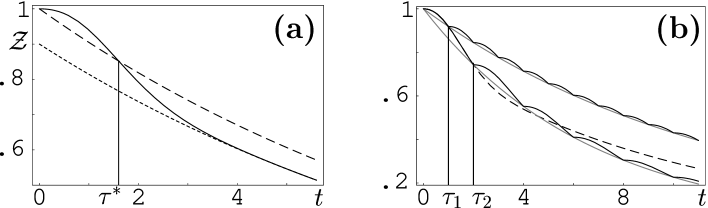
FIG. 1.: (a) Determination of $\tau^{*}$. The full line is the survival probability, the dashed line the exponential $e^{-\gamma_{0}t}$ and the dotted line the asymptotic exponential ${\cal Z}e^{-\gamma_{0}t}$ [see Eq. (10) in the following]. (b) Quantum Zeno vs inverse Zeno effect. The dashed line represents a typical behavior of the survival probability $P(t)$ when no measurement is performed: the short-time Zeno region is followed by an approximately exponential decay with a natural decay rate $\gamma_{0}$. When measurements are performed at time intervals $\tau$, we get the effective decay rate $\gamma(\tau)$. The full lines represent the survival probabilities and the dotted lines their exponential interpolations, according to (1). For $\tau_{1}<\tau^{*}<\tau_{2}$ the effective decay rate $\gamma(\tau_{1})$ [$\gamma(\tau_{2})$] is smaller (QZE) [larger (IZE)] than the “natural” decay rate $\gamma_{0}$. When $\tau=\tau^{*}$ one recovers the natural lifetime, according to (4).

We shall work in a quantum field theoretical framework. Consider the Hamiltonian ($\hbar=1$)

$$H=H_{0}+H_{\rm int}=\omega_{a}|a\rangle\langle a|+\int d\omega\;\omega|\omega\rangle\langle\omega|+\int d\omega\;g(\omega)(|a\rangle\langle\omega|+|\omega\rangle\langle a|),$$ (5)

where $\langle a|a\rangle=1,\langle a|\omega\rangle=0$ and $\langle\omega|\omega^{\prime}\rangle=\delta(\omega-\omega^{\prime})$. It describes the interaction of a normalizable (discrete) state $|a\rangle$ (the initial state) with a continuum of states $|\omega\rangle$ into which it can decay; $g(\omega)$ is the form factor of the interaction. The survival amplitude and probability of finding the system still in the initial state $|a\rangle$ at $t>0$ read

$$x(t)\equiv\langle a|\psi(t)\rangle,\qquad P(t)=|\langle a|\psi(t)\rangle|^{2}=|x(t)|^{2},$$ (6)

respectively, where $|\psi(t)\rangle$ is the state at time $t$, whose evolution is naturally restricted to the Tamm-Duncoff sector spanned by $\{|a\rangle,|\omega\rangle\}$. The survival amplitude is conveniently written as the inverse Fourier-Laplace transform of the propagator $x(E)=i\langle a|(E-H)^{-1}|a\rangle$,

$$x(t)=\int_{\rm B}\frac{dE}{2\pi}\;e^{-iEt}x(E),\qquad x(E)=\frac{i}{E-\omega_{a}-\Sigma(E)},$$ (7)

where the Bromwich path B is a horizontal line $\mbox{Im}E=$const$>0$ in the half plane of analyticity of the transform (upper half plane) and the self-energy function $\Sigma(E)$ is expressed in terms of the form factor

$$\Sigma(E)=\int d\omega\;\frac{\left|\langle a|H_{\rm int}|\omega\rangle\right|^{2}}{E-\omega}=\int d\omega\;\frac{g^{2}(\omega)}{E-\omega}.$$ (8)

A straightforward analysis in terms of the resolvent of the Hamiltonian yields

$$x(t)=\sqrt{{\cal Z}}e^{-\gamma_{0}t/2-i\alpha(t)}+x_{\rm cut}(t),\quad{\cal Z}=|1-\Sigma^{\prime}(E_{\rm pole})|^{-2}$$ (9)

where the exponential term (first term) is due to the contribution of a simple pole $E_{\rm pole}$ on the second Riemannian sheet in the complex energy plane, while the second term is the result of a contour integration [1]. The lifetime $\gamma_{0}^{-1}$ is given by the Fermi “golden” rule, computed according to the Weisskopf-Wigner approximation. The quantity ${\cal Z}$ is the square of the residue of pole of the propagator (wave function renormalization) and $\alpha$ a (real) linear function of time. The cut contribution is of order (coupling constant)² and modifies the exponential law both at short and long times, yielding the characteristic quadratic and power-law behaviors. The survival probability reads then

$$P(t)=|x(t)|^{2}={\cal Z}e^{-\gamma_{0}t}+\mbox{other terms}.$$ (10)

The above results are of general validity.

The following theorem holds: in general, a sufficient condition for the existence of a solution $\tau^{*}$ of Eq. (4) is ${\cal Z}<1$. The best proof of this proposition is obtained by graphical inspection: The case ${\cal Z}<1$ is shown in Fig. 1(a): $P(t)$ and $e^{-\gamma_{0}t}$ must intersect, since according to (10), $P(t)\sim{\cal Z}e^{-\gamma_{0}t}$ for large $t$ [9], and a finite solution $\tau^{*}$ can always be found. The other case, ${\cal Z}>1$, is shown in Fig. 2: a solution may or may not exist, depending on the model. Interestingly, the above theorem shows that renormalization plays an important role in the Zeno problem, when one deals with unstable systems.

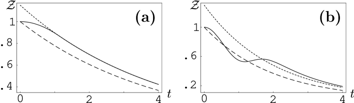
FIG. 2.: Study of the case ${\cal Z}>1$. The full line is the survival probability, the dashed line the renormalized exponential $e^{-\gamma_{0}t}$ and the dotted line the asymptotic exponential ${\cal Z}e^{-\gamma_{0}t}$. (a) If $P(t)$ and $e^{-\gamma_{0}t}$ do not intersect, a finite solution $\tau^{*}$ does not exist. (b) If $P(t)$ and $e^{-\gamma_{0}t}$ intersect, a finite solution $\tau^{*}$ exists. (In this case there are always at least two intersections.)

In order to check our general conclusions and investigate the primary role played by the specific features of the interaction, let us first focus on a Lorentzian form factor

$$g(\omega)=\frac{\lambda}{\sqrt{\pi}}\sqrt{\frac{\Lambda}{\omega^{2}+\Lambda^{2}}}.$$ (11)

This describes, for instance, an atom-field coupling in a cavity with high finesse mirrors [10] and has the advantage of being solvable. The role of form factors in the context of the QZE was studied in earlier papers [11, 12, 3]. In particular, Kofman and Kurizki also considered the Lorentzian case. (We stress that in this case the Hamiltonian is not lower bounded and we expect no deviations from exponential behavior at very large times, since Khalfin’s argument [13] is circumvented.) One easily obtains $\Sigma(E)=\lambda^{2}/(E+i\Lambda)$, whence the propagator $x(E)=i(E+i\Lambda)/[(E-\omega_{a})(E+i\Lambda)-\lambda^{2}]$ has two poles in the lower half energy plane and yields

$$x(t)=\frac{\omega_{a}+\Delta+i(\Lambda-\gamma_{0}/2)}{\omega_{a}+2\Delta+i(\Lambda-\gamma_{0})}e^{-i(\omega_{a}+\Delta)t}e^{-\gamma_{0}t/2}+\frac{\Delta-i\gamma_{0}/2}{\omega_{a}+2\Delta+i(\Lambda-\gamma_{0})}e^{i\Delta t}e^{-(\Lambda-\gamma_{0}/2)t},$$ (12)

where $\Delta=-\omega_{a}/2+(\omega_{a}/2)\sqrt{(\sqrt{\Omega^{4}+4\omega_{a}^{2}\Lambda^{2}}+\Omega^{2})/2\omega_{a}^{2}}$ and $\gamma_{0}=\Lambda-\sqrt{(\sqrt{\Omega^{4}+4\omega_{a}^{2}\Lambda^{2}}-\Omega^{2})/2}$, with $\Omega^{2}=\omega_{a}^{2}+4\lambda^{2}-\Lambda^{2}$. In this case the wave function renormalization reads

$${\cal Z}=\frac{(\omega_{a}+\Delta)^{2}+(\Lambda-\gamma_{0}/2)^{2}}{(\omega_{a}+2\Delta)^{2}+(\Lambda-\gamma_{0})^{2}}.$$ (13)

By plugging (12) into (3) one obtains the effective decay rate, whose behavior is displayed in Fig. 3 for different values of the ratio $\omega_{a}/\Lambda$.

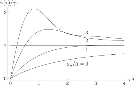
FIG. 3.: Effective decay rate $\gamma(\tau)$ for the model (11), for $\lambda=0.1$ and different values of the ratio $\omega_{a}/\Lambda$ (indicated). The horizontal line shows the “natural” decay rate $\gamma_{0}$: its intersection with $\gamma(\tau)$ yields the solution $\tau^{*}$ of Eq. (4). The asymptotic value of all curves is $\gamma_{0}$, as expected. A Zeno (inverse Zeno) effect is obtained for $\tau<\tau^{*}$ ($\tau>\tau^{*}$). Notice the presence of a linear region for small values of $\tau$ and observe that $\tau^{*}$ does not belong to such linear region as the ratio $\omega_{a}/\Lambda$ decreases. Above a certain threshold, given by Eq. (14) in the weak coupling limit of the model (and in general by the condition ${\cal Z}=1$), Eq. (4) has no finite solutions: only a Zeno effect is realizable in such a case.

These curves show that for large values of $\omega_{a}$ (in units $\Lambda$) there is indeed a transition from a Zeno to an inverse Zeno (“Heraclitus”) behavior: such a transition occurs at $\tau=\tau^{*}$, solution of Eq. (4). However, for small values of $\omega_{a}$, such a solution ceases to exist. The determination of the critical value of $\omega_{a}$ for which the Zeno–inverse Zeno transition ceases to take place discloses an interesting aspect of this issue. The problem can be discussed in general, but for the sake of simplicity we consider the weak coupling limit (small $\lambda$): in this case the other terms in (10), arising from the second addendum in (12), are of order $\lambda^{2}$ and quickly vanish for large $t$ ($\gamma_{0}$ is of order $\lambda^{2}$). Moreover, by (13) the inequality ${\cal Z}<1$ yields

$$\omega_{a}^{2}>\Lambda^{2}+\mbox{O}(\lambda^{2}).$$ (14)

The meaning of this relation is the following: a sufficient condition to obtain a Zeno–inverse Zeno transition is that the energy of the decaying state be placed asymetrically with respect to the peak of the form factor (bandwidth). If, on the other hand, $\omega_{a}\simeq 0$ (center of the bandwidth), no transition time $\tau^{*}$ exists (see Fig. 3) and only a QZE is possible: this is the case analyzed in Fig. 2(a). A relation similar to (14) was also discussed in [12].

There is more: Equation (12) yields a time scale. Indeed, from the definitions of the quantities in (12) one gets $\gamma_{0}/2<\Lambda-\gamma_{0}/2$, so that the second exponential in (12) vanishes more quickly than the first one [14]. If the coupling is weak, since $\gamma_{0}=\mbox{O}(\lambda^{2})$, the second term is very rapidly damped so that, after a short initial quadratic region of duration $\Lambda^{-1}$, the decay becomes purely exponential with decay rate $\gamma_{0}$. This is an important point, often misunderstood in the literature: the quadratic behavior $P(t)\simeq\exp(-t^{2}/\tau_{\rm Z}^{2})$ is valid not for times $t\lesssim\tau_{\rm Z}=\lambda^{-1}$, but rather for much shorter times $t\lesssim\Lambda^{-1}$. For $\tau\lesssim 1/\Lambda$ (which is, by definition, the meaning of “short” times in a quantum Zeno context), we can use the linear approximation

$$\gamma(\tau)\simeq\frac{\tau}{\tau_{\rm Z}^{2}}\quad\mbox{for}\quad\tau\lesssim 1/\Lambda,$$ (15)

where $\tau_{\rm Z}^{-2}\equiv\langle a|H_{\rm int}^{2}|a\rangle=\int d\omega g^{2}(\omega)$. When the linear approximation (15) applies up to the intersection (i.e., $|\omega_{a}|\gg\Lambda$) then

$$\tau^{*}\simeq\gamma_{0}\tau_{\rm Z}^{2}.$$ (16)

When the linear approximation does not hold, the r.h.s. of the above expression yields a lower bound to the transition time (4). The quantity $\gamma_{0}\tau_{\rm Z}^{2}$ is also relevant in different contexts and has been called “jump time” by Schulman [7].

The conclusions obtained for the simple model (11) are of general validity. Indeed, the form of the “rotating wave” interaction Hamiltonian (5) is a very general one [15]. In general, in Eq. (5), for any $g(\omega)$, we assume that $\omega_{a}>\omega_{g}$, where $\omega_{g}$ is the ground energy of the continuous spectrum, and regard $\omega$ as a collective index that can include some discrete variables (such as polarization in the case of photons), but must include at least a continuous one. The integral over $\omega$ is then a short notation for a sum over discrete quantum numbers and an integral over continuous ones. The matrix elements of the interaction Hamiltonian depend of course on the physical model considered. However, for physically relevant situations, the interaction smoothly vanishes for small values of $\omega-\omega_{g}$ and quickly drops to zero for $\omega>\Lambda$, a frequency cutoff related to the size of the decaying system and the characteristics of the environment. This is true both for cavities [10], as well as for typical EM decay processes in vacuum, where the bandwidth $\Lambda\simeq 10^{14}-10^{18}$s^-1 is given by an inverse characteristic length (say, of the order of Bohr radius) and is much larger than the (“natural”) inverse lifetime $\gamma_{0}\simeq 10^{7}-10^{9}$s^-1 [16].

For form factors that are roughly symmetric, all the conclusions drawn for the Lorentzian model remain valid. The main role is played by the ratio $\omega_{a}/\Lambda$. In general, the asymmetry condition (14) is satisfied if the energy $\omega_{a}$ of the unstable state is sufficiently close to the threshold. In fact, from the definition of the Zeno time $\tau_{\rm Z}$ one has

$$\frac{1}{\tau_{\rm Z}^{2}}=\int d\omega\;g^{2}(\omega)=g^{2}(\bar{\omega})\Lambda,$$ (17)

where $\bar{\omega}$ is defined by this relation and is of order $\omega_{\rm max}$, the energy at which $g(\omega)$ takes the maximum value. For $\omega_{a}$ sufficiently close to the threshold $\omega_{g}$ one has $g(\bar{\omega})\gg g(\omega_{a})$, the time scale $\gamma_{0}\tau_{\rm Z}$ is well within the short-time regime, namely

$$\gamma_{0}\tau_{\rm Z}^{2}=\frac{2\pi g^{2}(\omega_{a})}{g^{2}(\bar{\omega})\Lambda}\ll\frac{1}{\Lambda},$$ (18)

where the Fermi golden rule $\gamma_{0}=2\pi g^{2}(\omega_{a})$ has been used, and therefore the estimate (16) is valid.

On the other hand, for a system such that $\omega_{a}-\omega_{g}\simeq\Lambda$ (or, better, $\omega_{a}\simeq\;$center of the bandwidth), $\tau^{*}$ does not necessarily exist and usually only a Zeno effect can occur. In this context, it is useful and interesting to observe that the Lorentzian form factor (11) in (5) yields, in the limit $g^{2}(\omega)=\Lambda^{2}\delta(\omega-\omega_{a})$, the physics of a two level system. This is also true in the general case, for a roughly symmetric form factor, when the bandwidth $\Lambda\to 0$. In such a case, the physical conditions leading to QZE are readily realizable [17] (and no transition to IZE is possible).

Some final comments are in order. The present analysis has been performed in terms of instantaneous measurements, according to the Copenhagen prescription. Our starting point was indeed Eq. (1). We cannot help feeling that such a formulation of the QZE is unsatisfactory, even in the simplest case of two level systems [18]. A more exhaustive formulation, that takes into account the state of the detection system and the physical duration of the measurement process will be presented elsewhere. This approach, performed in terms of “continuous” measurements [19, 20, 7, 3, 5] circumvents the (very subtle) conceptual problem of state preparation, which affects most field theoretical formulations of the QZE. It is also worth emphasizing that the first experimental evidence of non-exponential decay at short times is very recent [21] and no hindered evolution due to repeated measurements (QZE) has ever been observed for bona fide unstable systems. The approach we propose might lead to new ideas for an experimental verification of these effects.

REFERENCES

- [1] H. Nakazato, M. Namiki and S. Pascazio, Int. J. Mod. Phys. B10, 247 (1996).
- [2] A. Beskow and J. Nilsson, Arkiv für Fysik 34, 561 (1967); L.A. Khalfin, Zh. Eksp. Teor. Fiz. Pis. Red. 8, 106 (1968) [JETP Letters 8, 65 (1968)]; B. Misra and E. C. G. Sudarshan, J. Math. Phys. 18, 758 (1977). For an updated review, see: D. Home and M.A.B. Whitaker, Ann. Phys. 258, 237 (1997).
- [3] S. Pascazio and P. Facchi, Acta Physica Slovaca 49, 557 (1999); P. Facchi and S. Pascazio, Phys. Rev. A62, 023804 (2000).
- [4] A.G. Kofman and G. Kurizki, Acta Physica Slovaca 49, 541 (1999); Nature 405, 546 (2000).
- [5] A. Luis and J. Peřina, Phys. Rev. Lett. 76, 4340 (1996); A. Luis and L. L. Sánchez–Soto, Phys. Rev. A57, 781 (1998); K. Thun and J. Peřina, Phys. Lett. A 249, 363 (1998); J. Řeháček et al, Phys. Rev. A62, 013804 (2000).
- [6] M. Lewenstein and K. Rza̧żewski, Phys. Rev. A61, 022105 (2000).
- [7] L.S. Schulman, Phys. Rev. A57, 1509 (1998).
- [8] P. Facchi and S. Pascazio, Phys. Lett. A241, 139 (1998); Physica A271 (1999) 133.
- [9] Namely, for times that are not too short (so that the cut contribution has become negligible) and not too long (so that no power low regime has taken over).
- [10] R. Lang, M.O. Scully and W.E. Lamb, Jr., Phys. Rev. A7, 1778 (1973); M. Ley and R. Loudon, J. Mod. Opt. 34, 227 (1987); J. Gea-Banacloche et al, Phys. Rev. A41, 381 (1990).
- [11] A.M. Lane, Phys. Lett. A99, 359 (1983).
- [12] A.G. Kofman and G. Kurizki, Phys. Rev. A54, R3750 (1996).
- [13] L. A. Khalfin, Dokl. Acad. Nauk USSR 115, 277 (1957) [Sov. Phys. Dokl. 2, 340 (1957)]; Zh. Eksp. Teor. Fiz. 33, 1371 (1958)[Sov. Phys. JETP 6, 1053 (1958)].
- [14] The two time scales become comparable only in the strong coupling regime: as .
- [15] Given any Hamiltonian and two projectors , the decomposition is always possible in terms of the diagonal operator and the off-diagonal one . The peculiarity lies in the fact that this description depends on the representation (namely, in our case, on the initial state ). See A. Peres, Ann. Phys. 129, 33 (1980). Such a decomposition remains valid in a general quantum field-theoretical framework: I. Joichi, Sh. Matsumoto and M. Yoshimura, Phys. Rev. D58, 043507; 045004 (1998). For additional subtle effects arising in quantum field theory see Ref. [8] and C. Bernardini, L. Maiani and M. Testa, Phys. Rev. Lett. 71, 2687 (1993); R.F. Alvarez-Estrada and J.L. Sánchez-Gómez, Phys. Lett. A253, 252 (1999).
- [16] H.E. Moses, Lett. Nuovo Cimento 4, 51; 54 (1972); Phys. Rev. A8, 1710 (1973); J. Seke, Physica A203, 269; 284 (1994).
- [17] R.J. Cook, Phys. Scr. T21, 49 (1988); W.H. Itano et al, Phys. Rev. A41, 2295 (1990).
- [18] A. Beige and G. Hegerfeldt, Phys. Rev. A53, 53 (1996); H. Nakazato et al, Phys. Lett. A217, 203 (1996); Z. Hradil et al, Phys. Lett. A239, 333 (1998).
- [19] K. Kraus, Found. Phys. 11, 547 (1981).
- [20] E. Mihokova, S. Pascazio and L.S. Schulman, Phys. Rev. A56, 25 (1997).
- [21] S.R. Wilkinson et al., Nature 387 (1997) 575.