Quantum Optimization

Abstract

We present a quantum algorithm for combinatorial optimization using the cost structure of the search states. Its behavior is illustrated for overconstrained satisfiability and asymmetric traveling salesman problems. Simulations with randomly generated problem instances show each step of the algorithm shifts amplitude preferentially towards lower cost states, thereby concentrating amplitudes into low-cost states, on average. These results are compared with conventional heuristics for these problems.

1 Introduction

Quantum computers [6, 7] operate on superpositions of all classical search states, allowing them to evaluate properties of all states in about the same time a classical machine requires for a single evaluation. This property is known as quantum parallelism. Superpositions are described by a state vector, consisting of complex numbers, called amplitudes, associated with the classical states.

Most quantum search algorithms focus on decision problems, which have an efficiently computable test of whether a given state is a solution. Without using any information about the problems beyond this test, quantum computers give a quadratic improvement in search speed by using amplitude amplification [11, 1]. Using more information gives further improvement in some cases [12, 13, 15, 27], but it remains to be seen how much improvement is possible for large, difficult search problems.

Some combinatorial searches have so many desired properties for a solution that none of the search states satisfy all of them, i.e., there is no solution. In such cases, one often instead asks for a state with as many desirable properties as possible [8]. More generally, each state has an associated cost and the goal is to find a minimum-cost state. Such optimization searches can be treated as a series of decision problems with different assumed values for the minimum cost. However many classical heuristics for optimization problems find low-cost states directly, although these are not guaranteed to be the actual minimum. This raises the question of whether quantum algorithms can show similar behavior since amplitude amplification does not directly apply to optimization problems where the minimum cost is not known a priori.

As a direct approach to optimizaton problems, this paper examines algorithms mixing amplitudes among different states so as to gradually shift the bulk of the amplitude toward states with relatively low costs, a technique previously applied to a decision problem [15]. Like many classical methods, the resulting quantum algorithms are heuristic (i.e., not guaranteed to find the minimum-cost state) and incomplete (i.e., even if such a state is found, the algorithm provides no definite indication that it is indeed a minimum). In common with most studies of heuristic methods, we evaluate their typical behavior on classes of problems rather than determining worst-case bounds (which are often far more pessimistic than typical behaviors). Specifically, the next section presents the quantum algorithm in the context of a general optimization problem, and contrasts it with amplitude amplification. The following two sections then examine instances of the algorithm suitable for overconstrained satisfiability problems (SAT) and asymmetric traveling salesman problems (ATSP).

2 Optimization Algorithm

The quantum optimization algorithm presented here operates on superpositions of all search states, and attempts to find a state with relatively low cost. The cost associated with each search state is used to adjust the phase of the state’s amplitude, and a mixing operation combines amplitudes from different states.

More specifically, the overall algorithm consists of a number of independent trials, each of which returns a single state after the final measurement. The number of trials can be fixed in advance if some (hopefully low-cost) state is required within a preset time bound, or can continue until some other criterion is satisfied, e.g., a sufficiently low cost state is found or a long series of trials gives no further improvement. In this respect, this algorithm is similar to incomplete classical heuristics which tend to give low-cost states but do not guarantee to find the absolute minimum. Moreover, even when the minimum is found, the algorithm offers no guarantee that this is indeed the minimum cost so that further trials will not give a lower cost.

2.1 A Single Trial

A single trial of the algorithm on a quantum computer with $n$ bits to represent the search state consists of the following efficiently implementable [1, 17] steps:

1. initialize the amplitude equally among the states, giving $\psi_{s}^{(0)}=2^{-n/2}$ for each of the $2^{n}$ states $s$.

2. for steps 1 through $j$, adjust amplitude phases based on the costs associated with the states and then mix them. These operations correspond to matrix multiplication of the state vector, with the final state vector given by:

   $$\psi^{(j)}=U^{(j)}P^{(j)}\ldots U^{(1)}P^{(1)}\psi^{(0)},$$ (1)

   where, for step $h$, $U^{(h)}$ is the mixing matrix and $P^{(h)}$ is the phase matrix, as described below.

3. measure the final superposition, giving state $s$ with probability $p(s)=|\psi^{(j)}_{s}|^{2}$. Thus the probability to obtain a minimum cost state with a single trial is ${P_{\rm min}}=\sum_{s}p(s)$ where the sum is over those $s$ with the minimum cost.

The mixing matrix is $U^{(h)}=WT^{(h)}W$, where, for states $r$ and $s$, $W_{rs}=2^{-n/2}(-1)^{|r\wedge s|}$ is the Walsh transform and $|r\wedge s|$ is the number of 1-bits the states have in common. The matrix $T^{(h)}$ is diagonal with elements depending on $|s|$, the number of 1-bits state $s$ contains: $T^{(h)}_{ss}=t^{(h)}_{|s|}$ with

$$t^{(h)}_{b}=e^{i\pi\tau_{h}b}$$ (2)

where $\tau_{h}$ is a constant depending on the class of problems and the number of steps, but not the particular problem instance being solved. From these definitions, the elements $U^{(h)}_{rs}$ depend only on the Hamming distance between the states, $d(r,s)$, i.e., the number of bits with different values in the two states. That is, we can write $U^{(h)}_{rs}=u^{(h)}_{d(r,s)}$, with $u^{(h)}_{d}=(-i\tan(\pi\tau_{h}/2))^{d}$, up to an overall phase and normalization constant [15].

The phase adjustment matrix, $P^{(h)}$, is a unitary diagonal matrix depending on the problem instance we’re solving, with values determined by the cost associated with each state: $P^{(h)}_{rr}=p^{(h)}_{c(r)}$ and

$$p^{(h)}_{c}=e^{i\pi\rho_{h}c}$$ (3)

where $\rho_{h}$ is a constant and $c(r)$ is the cost associated with search state $r$.

This algorithm has the same overall structure as amplitude amplification [11]. In fact, it reduces to amplitude amplification if we define the “cost” of a search state to be 0 for a solution and 1 otherwise and make the choices $t^{(h)}_{0}=-1$, $t^{(h)}_{b}=1$ for $b>0$, $p^{(h)}_{0}=-1$ and $p^{(h)}_{1}=1$ for all steps $h$. Note that for optimization problems where the minimum cost is not known a priori, none of the states will be solutions and amplitude amplification gives no enhancement in the minimum-cost states. On the other hand, the multiple trials of this optimization algorithm could be combined with amplitude amplification to achieve a further quadratic improvement if the minimum cost were known or through a series of repetitions using different assumed values for the minimum [2].

2.2 Applying the Algorithm

Completing the specification of the algorithm requires the number of steps $j$ and values for the phase parameters $\tau_{h}$ and $\rho_{h}$ for $h=1,\ldots,j$. We consider two approaches for identifying parameters giving good performance. The first uses a sample from the class of problems to be solved, and numerically adjusts the parameters to give the largest probability of finding a minimum cost state when averaged over the sample. This approach, commonly used to tune classical heuristics, allows precisely tuning the parameters but is limited to small problem sizes whose behavior can be simulated using classical machines. Applying this approach to larger problems will require the development of quantum hardware.

The second approach evaluates the asymptotic average behavior of the algorithm, as a function of the phase parameters, and selects values giving good average performance for large problems. When the number of steps $j$ is held fixed as $n$ increases, this can be done exactly [14]. However, good performance requires the number of steps to increase with the size of the problem, which complicates this exact analysis. Instead, we can use an approximate evaluation of the asymptotic behavior [15]. In this approximation, the amplitudes at each step are assumed to depend only on the costs associated with the states. Let $\phi^{(h)}_{c}$ be the average amplitude of states with cost $c$ after step $h$. With the above definitions of the mixing and phase matrices, the change in average amplitudes from one step to the next is approximately

$$\phi^{(h)}_{c^{\prime}}=\sum_{dc}u^{(h)}_{d}p^{(h)}_{c}\phi^{(h-1)}_{c}\nu(c^{\prime},d,c)$$ (4)

where $\nu(c^{\prime},d,c)$ is the average number of states with cost $c$ at distance $d$ from a state with cost $c^{\prime}$. This quantity can be expressed as ${n\choose d}P(c|d,c^{\prime})$ where $P(c|d,c^{\prime})$ is the conditional probability a state has cost $c$ when at distance $d$ from a state with cost $c^{\prime}$. When a class of problems has a simple expression for the asymptotic form of this conditional probability, this approximate equation gives the behavior of the average amplitudes. It can then be used to select phase parameters and the number of steps to give a large enhancement in amplitudes for low-cost states.

An optimization heuristc can be evaluated in a number of ways. For example, ${\left\langle C\right\rangle}=j/{P_{\rm min}}$ is the expected number of steps (including repetitions due to multiple trials) required to produce a minimum-cost state. Alternatively, one could ask how close the algorithm gets to the optimum as a function of the number of trials. This latter measure allows trade-offs between methods that give reasonably good results very quickly, but then give little subsequent improvement, and those that improve only slowly but eventually give lower cost states. Finally, one could characterize a single trial by its likelihood of returning the minimum cost, ${P_{\rm min}}$, or the expected cost of returned states, $\sum_{c}c\sum_{s|c(s)=c}p(s)$. In our case we focus on ${\left\langle C\right\rangle}$ as a performance measure. However, since the algorithms concentrate amplitude toward low-cost states, comparisons based on the other measures give the same general conclusions.

3 Satisfiability

Satisfiability is a combinatorial search problem consisting of a propositional formula in $n$ Boolean variables and the requirement to find an assignment (true or false) to each variable so that the formula is true. For $k$-satisfiability ($k$-SAT), the formula is a conjunction of $m$ clauses each of which is a logical OR of $k$ (possibly negated) variables. In this form, every clause must be true in order that the full formula is true. A state (i.e., an assigned value to each variable) is said to conflict with any clause it doesn’t satisfy. For $k\geq 3$, $k$-SAT is NP-complete [9]. An example 2-SAT problem with 3 variables and 2 clauses is ($v_{1}$ OR (NOT $v_{2}$)) AND ($v_{2}$ OR $v_{3}$), which has 4 solutions, e.g., $v_{1}={\rm false}$, $v_{2}={\rm false}$ and $v_{3}={\rm true}$.

$k$-SAT problems with many clauses typically have no solutions. Such cases give an optimization problem [8], namely to find assignments with the minimum number of conflicts, i.e., the fewest unsatisfied clauses. To examine typical behavior of the algorithm, we use the well-studied class of random $k$-SAT, in which the $m$ clauses are selected uniformly at random. Specifically, for each clause, a set of $k$ variables is selected randomly from among the $n\choose k$ possibilities. Then each of the selected variables is negated with probability $1/2$ to produce the clause. Thus each of the $m$ clauses is selected, with replacement, uniformly from among the ${n\choose k}2^{k}$ possible clauses. The difficulty of solving such randomly generated problems varies greatly from one instance to the next. This class has a high concentration of hard instances when $\mu\equiv m/n$ is near a phase transition in search difficulty [5, 21, 16]. For random 3-SAT this transition is near $\mu=4.25$. For our study of optimization, we generate these random problems but keep in the sample only those with no solutions, as evaluated with a classical exhaustive search. The minimum cost can vary among the instances in a sample.

3.1 Algorithm

Since SAT involves Boolean variables, the states in a problem with $n$ variables can be directly represented with $n$ bits in a quantum computer. With such a representation, the Hamming distance between two bit-sequences corresponds to the number of variables assigned different values in the two corresponding search states. This correspondence allows a simple combinatoric expression for the conditional probability $P(c|d,c^{\prime})$ that an assignment has $c$ conflicts when at distance $d$ from another assignment with $c^{\prime}$ conflicts. This expression can in turn be used to select algorithm parameters that lead to significant shift of amplitude toward states with few conflicts, on average [15].

Specifically, this approximation suggests using $j=n$ and a linear variation in the phase parameters, i.e., $\rho_{h}=\frac{1}{j}(R_{0}+R_{1}(1-\frac{h-1}{j}))$ and $\tau_{h}=\frac{1}{j}(T_{0}+T_{1}(1-\frac{h-1}{j}))$. Thus, for instance, the first step uses $\rho_{1}=(R_{0}+R_{1})/j$. As $j$ increases, the $\rho$ and $\tau$ values become small so the corresponding $P$ and $U$ matrices become close to identity matrices, i.e., each step only introduces small changes in the amplitudes.

The appropriate values of the four parameters, $R_{0}$, $R_{1}$, $T_{0}$ and $T_{1}$, depend on the class of SAT problems, in particular the values of $k$ and $\mu$ for random $k$-SAT. These values can be evaluated numerically in the context of decision problems, i.e., attempting to maximize the probability in solution states, assuming any exist [15]. This process gives parameter values suitable for problems with solutions. In this paper, we apply the same values for optimization problems.

3.2 Behavior

An example of the shift in amplitude is illustrated in Fig. 1. The distribution for step 0 simply reflects the number of states with each number of conflicts in the problem. Thus in this example most assignments have about 10 conflicts. Although this problem has no solutions, it shows the same shift in amplitude toward low-cost states as seen for soluble problems [15]. In particular, after the last step, the measurement is likely to produce a minimum-conflict state. Furthermore, even if such a state is not produced, the result is still very likely to have a relatively low number of conflicts. Significantly, the algorithm operates even without prior knowledge on the minimum number of conflicts. In fact, the approximate theory used to numerically select the phase parameters is based on maximizing the solution probability among soluble random 3-SAT with $\mu=4$ in this case. The figure shows such parameters also work well for insoluble problems. Thus the correlation between number of conflicts and Hamming distance used by the theory is roughly the same for soluble and insoluble instances for most of the states. Nevertheless, an open question is whether somewhat different phase parameters may give better performance for optimization problems.

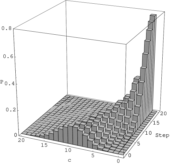
Figure 1: Probability to find an assignment with each number of conflicts vs. number of steps for a 3-SAT problem with 20 variables, 80 clauses and no solution (so the probability of finding a state with 0 conflicts is always zero). In this case, the minimum number of conflicts is one. The algorithm used $T_{0}=0.539298$, $T_{1}=3.5105$, $R_{0}=4$ and $R_{1}=-3.4$ with $j=20$ steps.

Classical heuristics also often manage to find low-conflict states. One such heuristic is GSAT [25]. The GSAT algorithm starts from a random assignment and, for each step, examines the number of conflicts in the assignment’s neighbors (i.e., assignments obtained by changing the value for a single variable) and moves to a neighbor with the fewest conflicts. If a solution isn’t found after a prespecified number of steps ($2n$ for the comparison reported here), e.g., because the current assignment is a local minimum, the search is tried again from a new random assignment. As with the quantum algorithm, GSAT is incomplete, i.e., does not guarantee its result is indeed a minimum-conflict assignment.

We use multiple trials to estimate the probability GSAT returns a minimum conflict state. Specifically, the expected cost estimate is ${\left\langle C\right\rangle}={S_{\rm total}}/{T_{\rm min}}$ where ${S_{\rm total}}$ is the total number of steps in all 1000 trials we used for each problem and ${T_{\rm min}}$ is the number of trials for which a minimum-conflict state was found.

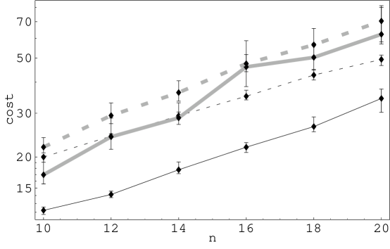
Figure 2: Median number of steps to find a state with the minimum number of conflicts, ${\left\langle C\right\rangle}=j/{P_{\rm min}}$, for random 3-SAT problems with $n$ variables and no solutions using $j=n$ steps for each trial. Solid curves show behavior for the quantum heuristic for $\mu=4$ (black) and 6 (gray). For comparison, the dashed curves show the corresponding behavior for the classical GSAT heuristic on the same problems. The algorithm used $T_{0}=0.539298$, $T_{1}=3.5105$, $R_{0}=4$ and $R_{1}=-3.4$ for $\mu=4$ and $T_{0}=0.87$, $T_{1}=2.7$, $R_{0}=2.57$ and $R_{1}=-1.73$ for $\mu=6$. The error bars show the 95% confidence interval for the median [26, p. 124]. The values are based on 100 problems for each $n$.

A comparison of the search costs, as measured by the expected number of steps, for GSAT and the quantum heuristic is shown in Fig. 2. Interestingly, the costs of the quantum algorithm are comparable or below those of GSAT. Actual search times for these methods will depend on detailed implementations of the steps. Although the number of elementary computational steps, involving evaluating the number of conflicts in an assignment (and, in the case of GSAT, its neighbors) are similar for both techniques, differences in the extent to which operations can be optimized and the relative clock rates of classical and quantum machines remain to be seen.

Since the trials of GSAT and this quantum heuristic are independent, decision problems allow a further quadratic speedup for either of these techniques by combining them with amplitude amplification [2]. Thus an interesting direction for future work is the extent to which such techniques, extended to use the number of conflicts in the search states, could give further improvement for optimization problems as well.

4 Traveling Salesman Problem

The asymmetric traveling salesman problem (ATSP) has $N$ cities with the distance from city $x$ to $y$ not necessarily equal to the distance from $y$ to $x$, as would be approriate, for instance, in planning routes along many one-way roads. The goal is a minimum-distance tour that visits every city exactly once and returns to the starting point. Many real-world planning and scheduling problems can be modeled as TSP’s [22, 23]. An $N$-city problem has $(N-1)!$ distinct tours starting and ending in a given city, and the time required to solve ATSP grows exponentially with $N$ [9].

We consider the average behavior for a class of TSPs studied in the context of phase transitions in search behavior [5, 29, 10]. Specifically, we looked at problems with intercity distances picked independently from a normal distribution with average $\mu$ and standard deviation $\sigma$, and then rounded to the nearest integer. Thus the probability a particular tour has length $L$ is a discretized normal distribution with average $N\mu$ and standard deviation $\sqrt{N}\,\sigma$. The value of $\mu$ just sets the distance scale: we take it equal to 100.

4.1 Algorithm

Quantum computers with $n$ bits are most naturally used with superpositions of $2^{n}$ classical states. Unlike the SAT problem, ATSP has no direct mapping between the $(N-1)!$ search states and the $2^{n}$ states representable by superpositions of $n$ quantum bits. Thus an important aspect of designing a quantum algorithm for this problem is selecting a suitable representation for the tours with binary elements.

One possibility, used in neural network approaches to TSP [18], represents each tour by a permutation matrix, i.e., an $N\times N$ matrix of binary values. Specifically, entry $i,j$ is one when city $i$ is at position $j$ in the tour. Thus a tour gives exactly one entry in each row and column that is equal to one, and the rest are zero. Since the choice of the first city is arbitrary, we can take city 1 to be the first in each tour, leaving a reduced $(N-1)\times(N-1)$ matrix describing the permutation of cities 2 through $N$. Such a matrix can be represented with $n=(N-1)^{2}$ binary values. While this representation has a fairly simple correspondence with the tours, considering superpositions of all $2^{n}$ possible values introduces many states that do not correspond to tours (i.e., cases in which the corresponding matrix has two or more 1’s in a single row or column and thus is not a permutation). Moreover, from a practical viewpoint, the quadratic growth in the number of bits with $N$ severely limits the problem sizes feasible for classical simulation. Thus, while this representation may be useful for theoretical analyses and may provide good performance, it is of limited use for empirically evaluating quantum heuristics on classical machines.

Another representation, requiring fewer bits, simply enumerates the tours starting from a given city in lexicographical order and associates each with a bit string representing its index in this list. For example, a 4-city problem with cities $A$, $B$, $C$, and $D$ has 6 distinct tours that start and end at city $A$: $ABCDA$, $ABDCA$, $ACBDA$, $ACDBA$, $ADBCA$, and $ADCBA$. Three bits are needed to represent these 6 tours, ranging from 000 to 101. The three bits give 8 possible values, so we also get 2 states without corresponding tours: 110 and 111.

Importantly for its use in a quantum algorith, the permutation corresponding to a given index can be computed efficiently as a particular example of techniques for ranking a variety of combinatorial structures [24]. Specifically, consider index $i$, ranging from 0 to $(N-1)!-1$, as specifying a permutation of cities 2 through $N$ (with the understanding that the overall tour starts and ends with city 1). The value ${\left\lfloor i/(N-2)!\right\rfloor}+2$, ranging from 2 to $N$, gives the first city in the permutation, and $i\bmod(N-2)!$ is the index of the permutation for the remaining cities. Repeating this procedure once for each city gives the full permutation in $O(N)$ operations.

This representation uses a number of states that is the closest power of two larger than or equal to the number of tours, i.e., $2^{n}\geq(N-1)!$, so $n={\left\lceil\log_{2}(N-1)!\right\rceil}\sim N\log_{2}(N/e)$. This introduces some extra states, not corresponding to tours, but far fewer than using the permutation matrix representation. The algorithm must operate so as to avoid giving much amplitude to these extra states.

For this problem, the phase adjustments depend on $c$, the scaled tour length: $c(r)=L(r)/(N\mu)$ (where $N\mu$ is the average tour length in this class of problems and $L(r)$ is the length of tour $r$, i.e., the sum of costs between successive cities in its path). Smaller values of $c$ correspond to shorter tours. This definition makes the behavior of this algorithm similar to that of the SAT algorithms described earlier, where $c$ represented the number of conflicts in an assignment. Since we want the extra states (the ones added to make the total number of states a power of two) to have small amplitudes, they should be assigned a large value of $c$. We chose $c=2$ for these extra states, so they are treated as additional tours with especially long lengths.

With this representation of the tours, the Hamming distance between two bit-strings has no simple relation to the difference of the corresponding tours. This precludes a simple expression for the conditional probability $P(c|d,c^{\prime})$ used in the approximate theoretical approach to identifying good phase parameters. Instead, we examined the performance for a random sample of problems, allowing for different values of these parameters at each step of the algorithm. We found only a small effect on performance from allowing $\tau_{h}$ to vary from one step to the next, so we take it to be a fixed value $\tau$ for the results reported below. However, using a different $\rho_{h}$ value for each step significantly improved performance. In particular, we took the values to vary linearly, as with the SAT algorithm, i.e., we took $\rho_{h}={\rho_{\rm init}}+{\rho_{\rm rate}}h$ for $h$ from 1 to $j$ where ${\rho_{\rm init}}$ and ${\rho_{\rm rate}}$ were new parameters depending only on the class of problems, defined by $\mu$ and $\sigma$, and total number of steps.

In summary, for given choices of $\mu$, $\sigma$ and total number of steps $j$, we selected parameters $\tau$, ${\rho_{\rm init}}$ and ${\rho_{\rm rate}}$ giving the best average performance based on evaluation with a sample of problems. The best choices we found for these parameters are listed and discussed in the next section.

4.2 Behavior

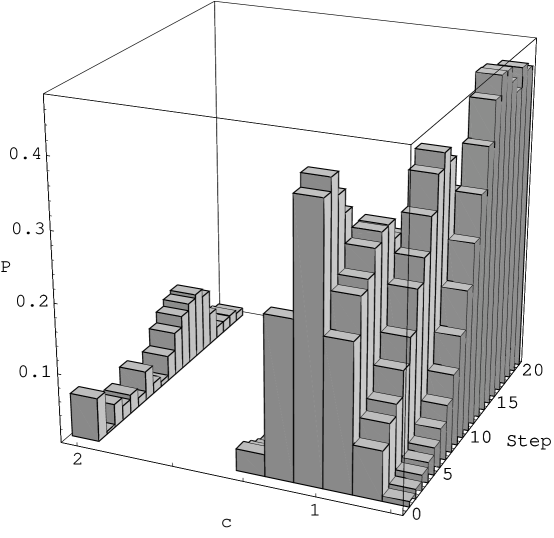
Figure 3: Probability to find a tour vs. scaled length $c$ and number of steps for a 6-city ATSP with $\mu=100$ and $\sigma=40$. Tours are binned according to their scaled lengths. The minimum tour, with $c=0.72$, is the only one in the bin with the smallest $c$ value. The bin at $c=2$ has the extra states that do not correspond to tours.

Fig. 3 illustrates the algorithm’s behavior for a random 6-city problem. The height of each bin is the sum of the probabilities $p(s)$ of all the tours $s$ whose lengths fall in the bin’s range. The initial step shows the initial distribution of tour lengths. We see the algorithm shifts amplitude from the longer tours towards shorter ones. For the problem instance shown in the figure, the probability of finding the optimal tour peaks at 0.45 after 16 steps. After 20 steps, the bins with large probabilities correspond to short tours. Thus when the algorithm does not find the optimal tour, it will most likely still produce a tour close to optimal. A similar shift toward shorter tours occurs for other problems including those with more cities.

To evaluate the average behavior for random 6- and 7-city problems we generated 100 problems with $\mu=100$ and $\sigma$ equal to 5, 10, 15, 20, 30, and 40, and then applied the algorithm for 20 steps. The results show the cost of solving the problems doesn’t depend on the $\sigma$ parameter of the distribution. In other words, all problems of a given size are equally complex; there are no hard and easy cases for this algorithm. This behavior differs from most classical heuristics that work particularly well on under- and overconstrained problems [10]. This difference indicates our algorithm is not taking full advantage of the problem structure, most likely due to the simple form of the mixing matrix and the representation of tours. It suggests an opportunity for improved performance by developing mixing matrices using problem structure, or using state representations where Hamming distance is a meaningful measure of tour similarity.

Quantitatively, after 20 steps a solution to 6-city problems is found with probability of roughly 30%. This decreases to about 11% for 7-city problems. Thus, while the size of the search space increases seven-fold, the cost goes up just by a factor of 3. With additional steps, the solution probability increases. For example, after 30 steps (with different optimal choices for the parameters $\tau$, ${\rho_{\rm init}}$ and ${\rho_{\rm rate}}$), a solution to an average 7-city problem with $\sigma=40\%$ is found with a probability of about 16%. Identifying the best number of steps, on average, remains an open question. In particular, based on the behavior of the algorithm for SAT, taking the number of steps proportional to $N$ may give better performance with suitable choices for the phase parameters.

deviation	5%	10%	15%	20%	30%	40%
6 cities
${\rho_{\rm init}}$	.32	.28	.36	.32	.32	.32
${\rho_{\rm rate}}$	.84	.44	.32	.24	.16	.12
$\tau$	.12	.12	.12	.12	.12	.12
7 cities
${\rho_{\rm init}}$	.36	.32	.36	.36	.36	.32
${\rho_{\rm rate}}$	.84	.44	.36	.24	.16	.12
$\tau$	.12	.12	.12	.12	.12	.12

Table 1: Optimal parameters for 20 steps.

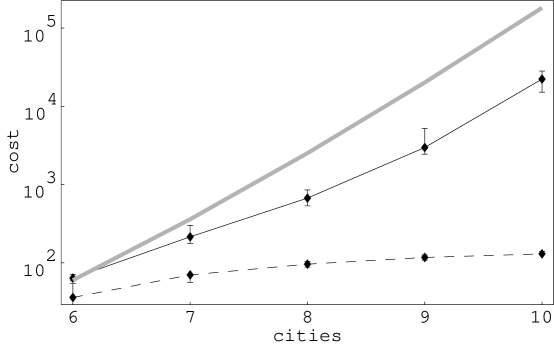
Figure 4: Median number of steps to find the optimal tour vs. $N$ for $\sigma=40\%$. The black curve shows the quantum search cost, $20/{P_{\rm min}}$, using the optimal parameters for 6 and 7 cities, which are identical in this case. The gray curve shows the scaling of random selection and the dashed curve is the cost estimate for the classical method DFBnB described in the text. The error bars show the 95% confidence intervals for the medians. Each point is based on a sample of 100 problems.

Table 1 summarizes the the phase parameters used in 6 and 7-city simulations, i.e., values of ${\rho_{\rm init}}$, ${\rho_{\rm rate}}$ and $\tau$ that maximize the probability of finding the optimal tour in 20 steps. The optimal $\rho^{(h)}={\rho_{\rm init}}+{\rho_{\rm rate}}h$ values are almost independent of the problem size, but are largely (and very consistently) dependent on $\sigma$: doubling $\sigma$ roughly halves the value of $\rho$. This is to be expected because doubling $\sigma$ also doubles the range of scaled tour lengths, $c-1$ (where 1 is the average value of $c$ for the class of problems). Thus halving $\rho$-values keeps the phase matrix entries $p_{c(r)}$ about the same, up to an irrelevant overall phase. Since the mixing matrix does not use the problem structure, it is not surprising that the optimal value of the mixing matrix constant $\tau$ is independent of $N$ and $\sigma$ for a given number of steps.

Fig. 4 shows the scaling behavior for a fixed choice of $\sigma$. For $N>7$, the simulations are too slow to allow finding optimal parameter values. Instead, noting the parameters for the 6 and 7 city problems, given in Table 1, were the same for $\sigma=40\%$, we continued using these parameters for the larger $N$. The solution probability after 20 steps decreases as $e^{-1.2N}$. These larger cases continue to show the shift of probability toward short tours. The resulting costs grow more slowly than the expected number of trials for random selection to find the optimal tour, $(N-1)!/2$. This random selection contrasts with exhaustive enumeration, with cost $(N-1)!$, which not only finds the optimum but also guarantees the result is indeed optimal.

As another comparison, Fig. 4 also shows an estimate of the median cost for a good classical method, depth-first branch-and-bound (DFBnB) [28]. This technique relies on the assignment problem (AP), in which each city is linked to another so that the total cost of these links is minimized. The resulting links need not form a complete tour, in which case the search proceeds by considering subproblems in which some of the links in the AP solution are not allowed. The initial AP can be solved in time of order $N^{3}$ while subsequent instances appearing in the subproblems require only $N^{2}$ operations. Ignoring overall constants and the, usually relatively minor, cost to find an initial upper bound on tour lengths by adjusting the result of the initial AP [19], we take the search cost associated with this method to be $C_{\rm classical}\approx N^{3}+bN^{2}$ where $b$ is the number of subproblems evaluated during the search. To compare with the quantum search cost measured in terms of steps, note that each step involves computing the cost of tours in superposition, which requires $O(N)$ operations. Thus we divide $C_{\rm classical}$ by $N$ to obtain the cost estimates used for comparison in Fig. 4. While the estimate does not include multiplicative constants, it does show the classical heuristic grows much more slowly than the quantum method introduced here. One caveat is that for large problems $b$ grows exponentially but for the small problems accessible to the quantum simulations, i.e., $N$ up to about 10, about a third of the instances are solved without any search since the initial assignment problem returns a complete tour. Many other cases are solved by expanding just a few subproblems. Thus many of these small problems are dominated by the cost of the initial AP and the figure does not show the eventual exponential growth in cost. We should also note this classical algorithm, unlike the quantum algorithm and GSAT, is complete and guarantees its result is indeed the minimum.

In spite of these limitations, this comparison does suggest the quantum technique is not particularly effective in exploiting problem structure, especially when compared with the satisfiability search described above. An interesting open question is whether this indicates quantum heuristics are inherently less effective for ATSP than for SAT. Other possible reasons for the relatively large costs with the quantum algorithm include the choice of problem representation, which does not explicitly use the relations among tours with many common edges, and nonoptimal values of phase adjustment parameters and number of steps for the larger problem sizes considered here.

5 Conclusion

A quantum algorithm shifting amplitude toward low-cost states is effective for combinatorial optimization problems, and does not require prior knowledge of the minimum cost for particular instances. This work illustrates how quantum techniques developed for decision problems can also apply to optimization, but only if they make use of the cost structure of the states. The experiments for satisfiability indicate appropriate phase parameters can allow the algorithm to have performance at least comparable to classical heuristics. The exponential increase in cost for classical simulation precludes evaluating these observations with larger problems.

For the asymmetric traveling salesman problem, our algorithm works fairly well for small instances, and specifically is much better than random selection. Its performance is independent of the standard deviation of the intercity distances. By allowing contributions from different search states to interfere, the algorithm avoids the large resource costs of using quantum parallelism without mixing the amplitudes [4]. One direction for future work is examining other ways of encoding the problem. Currently all the tours are enumerated in lexicographical order, and the mixing matrix doesn’t take advantage of the problem structure. Other enumerations may allow the mixing matrix to incorporate some problem structure. In analogy with the mixing of assignments in SAT, we could favor mixing amplitudes amongst similar tours, since tours that have a large number of edges in common are likely to have similar lengths. Ideally, such a representation could provide simple analytic evaluation of the conditional probability and thereby suggest better phase parameters for larger problems.

For some classical search methods applied to decision problems, the method can be incorporated in a quantum algorithm to give a further improvement [2, 3]. Hence an interesting open question is whether such techniques can generalize to optimization problems and thereby improve, for instance, on GSAT and the branch-and-bound examples of classical heuristics discussed here.

Unlike decision problems where results are easily verified, this optimization algorithm’s results cannot be directly checked for optimality. Thus, as with classical heuristics, such as GSAT and simulated annealing [20], applied to optimization problems, this algorithm does not indicate whether its result is indeed optimal. Moreover, although we focus on the probability to find the optimal tour, algorithms for optimization problems are characterized more generally by their trade-off between search cost and quality of the result. Such trade-offs may be particularly relevant for implementations of quantum computers limited to relatively few steps due to decoherence. For the algorithms considered here, the required number of coherent computational steps (i.e., the length of a single trial) grows at most linearly with with problem size. This contrasts with the exponentially growing number of steps in a single trial of amplitude amplification. Thus the structure-based algorithms make less stringent requirements on the extent to which coherence can be maintained.

In summary, we have shown how to use the cost associated with states in an optimization problem to adjust a superposition to increase the amplitudes associated with low-cost states. This opens a new direction for applying quantum computers to combinatorial searches, but the extent to which this capability can improve on classical heuristics, on average, remains an open question.

References

- [1] Michel Boyer, Gilles Brassard, Peter Hoyer, and Alain Tapp. Tight bounds on quantum searching. In T. Toffoli et al., editors, Proc. of the Workshop on Physics and Computation (PhysComp96), pages 36–43, Cambridge, MA, 1996. New England Complex Systems Institute.
- [2] Gilles Brassard, Peter Hoyer, and Alain Tapp. Quantum counting. In K. Larsen, editor, Proc. of 25th Intl. Colloquium on Automata, Languages, and Programming (ICALP98), pages 820–831, Berlin, 1998. Springer. Los Alamos preprint quant-ph/9805082.
- [3] Nicolas J. Cerf, Lov K. Grover, and Colin P. Williams. Nested quantum search and NP-complete problems. In Applicable Algebra in Engineering, Communication and Computing. Springer, Berlin, 1998. Los Alamos preprint quant-ph/9806078.
- [4] Vladimir Cerny. Quantum computers and intractable (NP-complete) computing problems. Physical Review A, 48:116–119, 1993.
- [5] Peter Cheeseman, Bob Kanefsky, and William M. Taylor. Where the really hard problems are. In J. Mylopoulos and R. Reiter, editors, Proceedings of IJCAI91, pages 331–337, San Mateo, CA, 1991. Morgan Kaufmann.
- [6] D. Deutsch. Quantum theory, the Church-Turing principle and the universal quantum computer. Proc. R. Soc. London A, 400:97–117, 1985.
- [7] David P. DiVincenzo. Quantum computation. Science, 270:255–261, 1995.
- [8] Eugene C. Freuder and Richard J. Wallace. Partial constraint satisfaction. Artificial Intelligence, 58:21–70, 1992.
- [9] M. R. Garey and D. S. Johnson. Computers and Intractability: A Guide to the Theory of NP-Completeness. W. H. Freeman, San Francisco, 1979.
- [10] Ian P. Gent, Ewan MacIntyre, Patrick Prosser, and Toby Walsh. The scaling of search cost. In Proc. of the 14th Natl. Conf. on Artificial Intelligence (AAAI97), pages 315–320, Menlo Park, CA, 1997. AAAI Press.
- [11] Lov K. Grover. Quantum mechanics helps in searching for a needle in a haystack. Physical Review Letters, 78:325–328, 1997. Los Alamos preprint quant-ph/9706033.
- [12] Lov K. Grover. Quantum search on structured problems. Chaos, Solitons, and Fractals, 10:1695–1705, 1999.
- [13] Tad Hogg. Highly structured searches with quantum computers. Physical Review Letters, 80:2473–2476, 1998. Preprint at publish.aps.org/eprint/gateway/eplist/aps1997oct30_002.
- [14] Tad Hogg. Single-step quantum search using problem structure. Los Alamos preprint quant-ph/9812049, 1998.
- [15] Tad Hogg. Quantum search heuristics. Physical Review A, 61:052311, 2000. Preprint at publish.aps.org/eprint/gateway/eplist/aps1999oct19_002.
- [16] Tad Hogg, Bernardo A. Huberman, and Colin P. Williams, editors. Frontiers in Problem Solving: Phase Transitions and Complexity, volume 81, Amsterdam, 1996. Elsevier. Special issue of Artificial Intelligence.
- [17] Tad Hogg, Carlos Mochon, Eleanor Rieffel, and Wolfgang Polak. Tools for quantum algorithms. Intl. J. of Modern Physics C, 10:1347–1361, 1999. Los Alamos preprint quant-ph/9811073.
- [18] J. J. Hopfield and D. W. Tank. “Neural” computation of decisions in optimization problems. Biol. Cybern, 52:141–152, 1985.
- [19] Richard M. Karp. A patching algorithm for the nonsymmetric traveling-salesman problem. SIAM J. on Computing, 8:561–573, 1979.
- [20] S. Kirkpatrick, C. D. Gelatt, and M. P. Vecchi. Optimization by simulated annealing. Science, 220:671–680, 1983.
- [21] Scott Kirkpatrick and Bart Selman. Critical behavior in the satisfiability of random boolean expressions. Science, 264:1297–1301, 1994.
- [22] E. L. Lawler, J. K. Lenstra, A. H. G. Rinnooy Kan, and D. B. Shmoys, editors. The Traveling Salesman Problem. John Wiley, NY, 1985.
- [23] Donald L. Miller and Joseph F. Pekny. Exact solution of large asymmetric traveling salesman problems. Science, 251(4995):754–761, Feb. 15 1991.
- [24] A. Nijenhuis and H. S. Wilf. Combinatorial Algorithms for Computers and Calculators. Academic Press, New York, 2nd edition, 1978.
- [25] Bart Selman, Hector Levesque, and David Mitchell. A new method for solving hard satisfiability problems. In Proc. of the 10th Natl. Conf. on Artificial Intelligence (AAAI92), pages 440–446, Menlo Park, CA, 1992. AAAI Press.
- [26] George W. Snedecor and William G. Cochran. Statistical Methods. Iowa State Univ. Press, Ames, Iowa, 6th edition, 1967.
- [27] Lee Spector, Howard Barnum, Herbert J. Bernstein, and Nikhil Swamy. Finding a better-than-classical quantum AND/OR algorithm using genetic programming. In P. Angeline, editor, Proc. of the 1999 Congress on Evolutionary Computing, Washington, DC, 1999. IEEE.
- [28] Weixiong Zhang. Depth-first branch-and-bound versus local search: A case study. In Proc. of the 17th Natl. Conf. on Artificial Intelligence (AAAI2000). AAAI, 2000.
- [29] Weixiong Zhang and Richard E. Korf. A study of complexity transitions on the asymmetric traveling salesman problem. Artificial Intelligence, 81:223–239, 1996.